Turbulent flow separation in three-dimensional
asymmetric diffusers
Elbert Jeyapaul
Iowa State University
Follow this and additional works at:
https://lib.dr.iastate.edu/etd
Part of the
Aerospace Engineering Commons
This Dissertation is brought to you for free and open access by the Iowa State University Capstones, Theses and Dissertations at Iowa State University Digital Repository. It has been accepted for inclusion in Graduate Theses and Dissertations by an authorized administrator of Iowa State University Digital Repository. For more information, please [email protected].
Recommended Citation
Jeyapaul, Elbert, "Turbulent flow separation in three-dimensional asymmetric diffusers" (2011).Graduate Theses and Dissertations. 10258.
by
Elbert Jeyapaul
A dissertation submitted to the graduate faculty in partial fulfillment of the requirements for the degree of
DOCTOR OF PHILOSOPHY
Major: Aerospace Engineering
Program of Study Committee: Paul A. Durbin, Major Professor
Zhi J. Wang Hui Hu Alric P. Rothmayer
James C. Hill
Iowa State University Ames, Iowa
2011
TABLE OF CONTENTS LIST OF TABLES . . . iv LIST OF FIGURES . . . v NOMENCLATURE . . . x ACKNOWLEDGEMENTS . . . xii ABSTRACT . . . xiii CHAPTER 1. OVERVIEW . . . 1 1.1 Separation definition . . . 2 1.2 Background . . . 3 1.3 Asymmetric diffuser . . . 4
1.4 Reynolds number dependence . . . 6
1.5 Outline of the Thesis . . . 6
CHAPTER 2. DIFFUSER SERIES . . . 8
2.1 Quasi 1-D analysis . . . 8
2.2 Computational model . . . 11
2.2.1 Codes and Numerics . . . 12
2.2.2 Inflow profile generation . . . 14
2.2.3 Computing resources . . . 15
CHAPTER 3. EDDY-RESOLVING SIMULATIONS . . . 16
3.1 Detached Eddy Simulations . . . 16
3.1.1 Validation . . . 18
3.1.3 Vortical flow features . . . 22
3.2 Large Eddy Simulations . . . 24
3.2.1 Verification . . . 27
3.2.2 Diffuser series . . . 30
3.3 Comparison of LES and DES . . . 35
CHAPTER 4. SINGLE POINT CLOSURE MODELS . . . 38
4.1 Linear eddy-viscosity models (LEVM) . . . 38
4.1.1 Anomalies in predicting 3-D separation . . . 39
4.2 Sensitizing Cµ to flow separation . . . 42
4.2.1 Modeling parameters . . . 43
4.3 Importance of Anisotropy . . . 46
4.4 Anisotropy-resolving models . . . 46
4.5 Explicit Algebraic Reynolds Stress Model(EARSM) . . . 49
4.5.1 Formulation . . . 50
4.5.2 Implementation and Numerics . . . 51
4.5.3 Diffuser flow prediction . . . 52
4.5.4 Mean flow comparison . . . 53
4.5.5 Comparison of Reynolds stress . . . 55
4.5.6 Separation in the diffuser family . . . 55
4.5.7 General quasi-linear model . . . 56
4.5.8 Square duct prediction . . . 56
4.5.9 EARSM variants . . . 61
CHAPTER 5. CONCLUSION . . . 66
5.1 Future work . . . 67
LIST OF TABLES
Table 2.1 Family of diffusers generating same adverse pressure gradient . . . 10 Table 2.2 Computational resource for each Eddy-resolving and RANS simulation 15
Table 4.1 ARSM coefficients for different linear Πrij models . . . 59 Table 4.2 ARSM coefficients for the calibrated LRR and other linear Πij models 64
LIST OF FIGURES
Figure 1.1 Dimensions of Cherry’s diffuser 1 (Cherry et al., 2008) . . . 5 Figure 2.1 Area distribution(a) and streamwise pressure gradient(b) used in
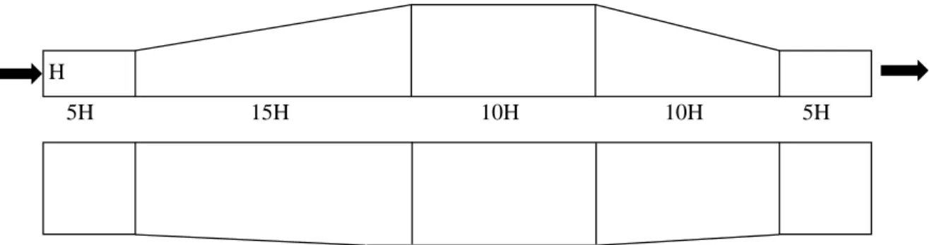
gen-erating the diffuser series . . . 10 Figure 2.2 Outline of the diffuser domain used for simulations. Shown in side and
top view. . . 11 Figure 2.3 Mesh distribution in the diffuser showing every 4th node. . . 12 Figure 2.4 Flow domain with inlet mapping . . . 14 Figure 2.5 Primary and Secondary velocity profile in the fully-developed
rectangu-lar channel of A=3.33. Statistics were averaged over 50 flow-through times. . . 15
Figure 3.1 Power spectrum of instantaneous streamwise velocity. The 4 probe points are located at the centroid of cross-sectional planes that are equally spaced from inlet to outlet. The -5/3 slope line is in red. . . . 17 Figure 3.2 The ratio of the resolved-to-modeled turbulent energy in the baseline
diffuser DES. . . 18 Figure 3.3 Streamwise velocity predicted using SAS and experimental
measure-ments of Cherry et al. (2006) at transverse planes. Contour lines are spaced 0.1 m/s apart. The zero-streamwise-velocity contour line is thicker than the others. . . 19 Figure 3.4 Variation of mean streamwise velocity along spanwise z-lines. B is the
width of the diffuser at that x-location. The solid lines are DES, and dashedk−ω SST model compared with experimental data. . . 20
in red. . . 21 Figure 3.6 Separation bubble(a) and Intermittency(b) in the A2.5 diffuser
pre-dicted using the DES model. . . 22 Figure 3.7 Secondary flow show a similarity in pattern at different inlet aspect
ra-tios. The foci is formed earlier in theA2.5 diffuser and moves downstream 22 Figure 3.8 (a)Limiting streamlines forA2.5 diffuser on the wall show a steady
sepa-ration surface from the top wall, The side wall has a complex sepasepa-ration- separation-attachment flow. (b)The vortex cores show a vortex originating from foci F3 on left and multiple vortices close to the double-sloped edge . . 23 Figure 3.9 Secondary flow streamlines in transverse planes of A2 diffuser. The
blue line indicates the location of separation surface. . . 24 Figure 3.10 Power spectrum of instantaneous streamwise velocity predicted by LES.
The 4 probe points are located at the centroid of cross-sectional planes that are equally spaced from inlet to outlet. The -5/3 slope line is in red. 26 Figure 3.11 The quality of the LES assessed using the metric of (a) Ratio of resolved
to total Turbulent kinetic energy and (b)LES IQν parameter . . . 27 Figure 3.12 Contour lines of mean streamwise velocity and streamwise RMS velocity
at various transverse planes. The DNS is to the left and LES on the right on each of Figures (a) and (b). Each line is spaced by 0.1 and the zero velocity line is bold. . . 28 Figure 3.13 Comparison of mean flow velocities, resolved kinetic energy, and Reynolds
stresses alongz/B=1/2by LES of baseline diffuser. DNS are solid and LES are dashed. . . 31 Figure 3.14 Comparison of mean flow velocities, resolved kinetic energy, and Reynolds
stresses alongz/B=1/4by LES of baseline diffuser. DNS are solid and LES are dashed. . . 32
Figure 3.15 Comparison of mean flow velocities, resolved kinetic energy, and Reynolds stresses alongz/B=3/4by LES of baseline diffuser. DNS are solid and LES are dashed. . . 33 Figure 3.16 Comparison of mean flow velocities, resolved kinetic energy, and Reynolds
stresses alongz/B=7/8by LES of baseline diffuser. DNS are solid and LES are dashed. . . 34 Figure 3.17 Coefficient of pressure
Cp = p −pref 0.5ρU2 bulk
variation along the bottom wall of baseline diffuser predicted by LES, x/L is the non-dimensional diffuser length. The experimental Cp has been shifted by -0.02 to provide a better comparison. . . 35 Figure 3.18 Separation surface predicted by LES for the diffuser series . . . 35 Figure 3.19 Secondary flow predicted by LES at the diffuser exit plane x/H=15 of
the diffuser series. The cross-sections are shown in different scale, in real the areas are same. . . 36 Figure 3.20 Fraction of cross-sectional area separated predicted by DES and
Exper-iments for the baseline diffuser . . . 37
Figure 4.1 Primary and secondary flow predicted using thek−ω SST model. The transverse velocity in (b) is normalized byUbulk . . . 40 Figure 4.2 Separation surface predicted by SST model in the series of diffusers. . 41 Figure 4.3 Anomalous separation surface predicted by SST in diffusers with
sym-metric side slope angles. . . 42 Figure 4.4 Sensitivity of 2-D diffuser flow separation to variations inCµvalue. The
separation line is in bold. . . 43 Figure 4.5 Scatter of Eigen values of Velocity gradient tensor predicted by SST and
SAS models for the baseline diffuser. . . 44 Figure 4.6 Contours of Helicity in transverse plane of baseline diffuser predicted by
along mid-plane of diffuser z/B=0.5(b) The complete Reynolds stress tensoruiuj plotted at x/H=4 at diffuser midplane (z/B=0.5) . . . 47 Figure 4.9 A plot ofaij invariants at various streamwise locations (x/H) from DNS
results . . . 47 Figure 4.10 Variation of Reynolds stress anisotropy(aij) invariants along the span
of the baseline diffuser midplane (z=0.5B) from DNS results . . . 48 Figure 4.11 Secondary flow predicted by DNS and comparison to BEARSM. The
magnitudes of the Mean or secondary flow are colored. The streamlines do not show direction. . . 54 Figure 4.12 Secondary flow predicted by DNS and BEARSM at diffuser exist x/H=15.
The flow indicate the presence of 4 vortices. . . 54 Figure 4.13 Visualization of 3-D flow invariants from LES of baseline diffuser.
Re-gions of 0 have no 3D influence on anisotropy. . . 55 Figure 4.14 Separation topology in the family of diffusers predicted using an
anisotropy-resolving BEARSM and LES . . . 57 Figure 4.15 Streamwise mean velocity contours in the family of diffusers predicted
by BEARSM and LES. . . 58 Figure 4.16 Pressure on bottom wall predicted by the BEARSM and LES. The
ab-scissa is non-dimensionalized by diffuser length. . . 59 Figure 4.17 Separation predicted by two generalized linear EARSM. . . 59 Figure 4.18 Secondary flow magnitude (V) and Turbulent kinetic energy (k)
pre-dicted by EARSM and compared with DNS data. . . 60 Figure 4.19 Flow predicted in the baseline diffuser using the diffusion-corrected
EARSM . . . 62 Figure 4.20 Flow predicted in the baseline diffuser using Generalized linear model
Figure 4.21 WallCp predicted by different Generalized EARSM models . . . 65 Figure 5.1 Stress-strain lag parameter Cas = −√a2ijSSij
ijSij
evaluated from LES flow field of baseline diffuser. . . 69
p static pressure
x streamwise distance
ρ DensityVariable value vector
Q Flow rate, m3/s
A Cross sectional area, m2
α tangent of top flare angle
β tangent of side flare angle
Cµ Coefficient of eddy–viscosity
Cp Coefficient of pressure
S Non-dimensional strain tensor
A Aspect ratio
aij,a Turbulence anisotropy tensor
uiuj Reynolds stress tensor
U,V,W Mean flow velocity components u,v,w Fluctuating velocity components
Subscripts
sgs Subgrid Scale
r Reference diffuser
0 diffuser inlet
+ Non-dimensional wall units
x,y,z Cartesian coordinates
Greek symbols
δij Kronecker delta
κ Von Karman constant
τij Stress tensor
P/ε Production-to-dissipation ratio
ν Kinematic viscosity
α,β Tangents of top and side flare angles
βi Scalar coefficient of tensor polynomial basis ‘i’
Ω Non-dimensional vorticity tensor
Abbreviation
SST Shear Stress Transport
DES Detached Eddy Simulation
LES Large Eddy Simulation
SAS Scale Adaptive Simulation
RANS Reynolds–Averaged Navier Stokes
Firstly, I would like to thanks my advisor Dr. Paul Durbin for his guidance, patience and continued support of my doctoral research. His insightful thoughts and depth of knowledge has enriched my understanding on the subject of turbulence and inspired me to pursue research. Secondly, the financial support though NASA cooperative agreement NNX07AB29A and the Department of Aerospace Engineering is acknowledged. I would like to thank Postdoctoral scholars, Dr. Jongwook Joo for his help in using the code SuMB and Dr. Alberto Passalacqua for his guidance on OpenFOAM. Computational support for the simulations by Dr. James Coyle and John Dickerson has been timely and helpful. Without the allocation of NSF’s Teragrid cluster the large simulations could not be completed.
My stay at office has been lively sharing spaces with Jason Ryon and Sunil Arolla. I am thankful to graduate secretary Ms. Delora Pfeiffer for her help. It has been a privilege to be part of campus organizations Sankalp and Aerospace Engineering Graduate students’ organization. I have been fortunate to have many friends who have made my stay at Iowa state enjoyable. My uncle Dr. Jeyasingh Nithianandam and his family have been a source of encouragement. Finally, I thank my parents for their patience and encouragement in this endeavor.
ABSTRACT
Turbulent three-dimensional flow separation is more complicated than 2-D. The physics of the flow is not well understood. Turbulent flow separation is nearly independent of the Reynolds number, and separation in 3-D occurs at singular points and along convergence lines emanating from these points. Most of the engineering turbulence research is driven by the need to gain knowledge of the flow field that can be used to improve modeling predictions. This work is motivated by the need for a detailed study of 3-D separation in asymmetric diffusers, to understand the separation phenomena using eddy-resolving simulation methods, assess the predictability of existing RANS turbulence models and propose modeling improvements. The Cherry diffuser has been used as a benchmark. All existing linear eddy-viscosity RANS models
k−ωSST,k−andv2−f fail in predicting such flows, predicting separation on the wrong side.
The geometry has a doubly-sloped wall, with the other two walls orthogonal to each other and aligned with the diffuser inlet giving the diffuser an asymmetry. The top and side flare angles are different and this gives rise to different pressure gradient in each transverse direction. Eddy-resolving simulations using the Scale adaptive simulation (SAS) and Large Eddy Simulation (LES) method have been used to predict separation in benchmark diffuser and validated. A series of diffusers with the same configuration have been generated, each having the same streamwise pressure gradient and parametrized only by the inlet aspect ratio. The RANS models were put to test and the flow physics explored using SAS-generated flow field. The RANS model indicate a transition in separation surface from top sloped wall to the side sloped wall at an inlet aspect ratio much lower than observed in LES results. This over-sensitivity of RANS models to transverse pressure gradients is due to lack of anisotropy in the linear Reynolds stress formulation. The complexity of the flow separation is due to effects of lateral straining, streamline curvature, secondary flow of second kind, transverse pressure gradient on turbulence. Resolving these effects is possible with anisotropy turbulence models as the Explicit
pressure. There exists scope for improvement of this model, by including convective effects and dynamics of velocity gradient invariants.
CHAPTER 1. OVERVIEW
Aerodynamic flows are mostly streamlined and characterized by large irrotational regions, in which motion is dictated by a balance between convection and pressure gradients and a relatively thin rotational layer. Turbulent mechanisms play an important role only in the highly sheared regions such as boundary layers, wakes and separated mixing layers. While the fundamental turbulence mechanisms are complex even in attached flows, the engineer is only interested in a few global manifestations of turbulence, that are dictated by a statistical tur-bulence variables. This focus allows highly simplified turtur-bulence modeling approaches, such as the eddy viscosity. These models side-step the underlying physics and rely heavily on empirical correlations and constants derived from basic idealized flows. Flows in which turbulence plays a more influential role than in boundary layers require refined turbulence modeling. Among these are turbulent flow separation and recirculation caused due to adverse pressure gradients. Separations often occur at the limits of the design envelope and cause a loss in performance; hence it is of much interest to turbulence modeling research.
Separation can be induced by adverse pressure gradient or by geometric singularity; the former is discussed in this thesis. Turbulent separation is characterized by increased strain rates and higher production-to-dissipation (P/ε) ratio. Two-dimensional separation is well understood and most eddy-viscosity models produce accurate prediction of wall shear stress and pressure in up to moderate strain rates. At high strain rates, the log region of the boundary layer deviates from equilibrium, i.e. P/ε1, which makes the Reynolds stress-intensity ratio to be greater thanpCµ, hence standard eddy-viscosity models fail. This shortcoming was fixed in k-ω SST model by Menter (1994) using a stress limiter in the eddy-viscosity calculation. Three-dimensional separation is more complicated than in 2-D.
3-dent of the Reynolds number. A number of experiments have been conducted to study 3-D flow separation, notably are asymmetric diffuser (Cherry et al., 2008) and flow over a hill (Byun and Simpson, 2006, NASA Fundamental Aerodynamic Investigation of The Hill experiment). These are smooth wall separations, induced by APG and Reynolds stress anisotropy, unlike separa-tion separasepara-tion due to obstrucsepara-tion — as in wing-body juncsepara-tion or cross-flow separasepara-tion over a prolate spheroid or afterbody separation. In these flows, interacting 3-D turbulent boundary layers play an important role in creating secondary flow effects of second kind. As opposed to external flow, internal flow separation is more influenced by these secondary effects due to Reynolds stresses and only models that resolve secondary effects succeed in accurately predict-ing 3-D separation. Cherry’s diffuser has proven a challenge to linear eddy-viscosity models, which predict separation on the wrong wall of the diffuser, hence topologically incorrect. Engi-neering turbulence research today is driven by the need to gain knowledge that can be used to improve modeling predictions. The thesis work is motivated by the need for a detailed study of 3-D separation in diffusers, to understand the separation phenomena and propose modifications to improve the predictability of Reynolds-Averaged Navier Stokes (RANS) turbulence models.
1.1 Separation definition
Separation is the entire process of departure, or breakaway, of the boundary layer from a wall; or the breakdown of the boundary layer assumption. The separation surface is the surface that bounds the zone between the separated shear layer and the wall. Researchers have studied turbulent separation over the years, but each with a different definition of the separation surface/line. Hence there is need for a unified definition of separation line/surface. A collection of these definitions presented in T¨ornblom (2006), are;
• recirculation region with dividing streamline connecting stagnation points on wall.
• region with backflow more than 50% of the time (Simpson, 1989)
Here the locus of zero Streamwise velocity is adopted, as the average flow field is steady. Turbulent flow separation is best identified at the wall, rather than within the flow field, as the flow becomes two dimensional. Simpson (1996) defines the kind of separation from the percentage of time the wall shear stress reverses sign. An intermittent transitory detachment is whenτwall reverses sign 20% of time and detachment is whenτwall= 0, which is the case in the diffusers studied. Only pressure-induced separation occurs in diffusers, due to the gradual expansion.
1.2 Background
Though three-dimensional separated flow is highly chaotic and no straight forward extension exists from 2-D separation concepts, there has been a number of efforts to develop a rational approach to analyze these flows. Experimentalist rely more on wall stress signature (oil streaks) to characterize separation, and the mean flow streamlines in the bulk flow to analyze the vortex structures (D´elery, 2001). Legendre (1956) proposed analyzing the wall stresses using the geo-metric theory of two-dimensional smooth vector fields: one locates the zeros, singular/critical points of the skin friction field, identifies their stability type, then constructs the phase portrait of skin-friction trajectories. This critical point based approach has been adopted and extended by Tobak and Peake (1982), Chapman and Yates (1991) and Chong et al. (1990). In a general view, Lighthill (1963) proposed that convergence of skin friction lines is a necessary criterion for separation. He went on to deduce that separation lines always start from saddle-type skin-friction zeros and terminate at stable spirals or nodes. A review of terminologies and separation topologies are given in D´elery (2001). Haimes and Kenwright (1999) have used critical point theory and extended it to analyze velocity gradient of the flow to extract features. Feature extraction studies have been quite helpful in knowing separation flow features and topologies and also the vortex cores though Eigen analysis of the vorticity tensor. Recently, an extended description of three-dimensional steady flow separation has been developed by Surana et al. (2006) using wall stress lines.
mean flow and Reynolds stresses. Studies in 2-D planar diffusers primarily use the data set of Obi et al. (1993), which was repeated and extended by Buice and Eaton (2000). Obi et al. (1993) used a high aspect ratio inlet to eliminate the 3-D effect.
However as the inlet aspect ratio is reduced to about 4:1, a 3-D separation bubble begins to form. Experiments in 3-D asymmetric diffuser first performed by Cherry et al. (2008) indicate the separation behavior to be very sensitive to minor geometric changes. In their work, two doubly-sloped diffusers were tested at a Reynolds number of 10,000 based on inlet half height. Both diffusers have the same inlet cross-sectional area and aspect ratio, and the the same length and outlet areas that differed by less than 6%,; nevertheless, their separation bubbles developed very differently. The first diffuser has been used as a benchmark at a workshop1, as RANS models fail miserably for this case. Most of the researchers studied the flow using eddy-resolving simulations; Breuer et al. (2009) studied the flow using a Hybrid LES-RANS(HLR) with EARSM formulation in RANS regions. A similar simulation approach was used by Abe and Ohtsuka (2010); Gross and Fasel (2010), Uribe et al. (2010) used the SAS model. LES using the dynamic Smagorinsky model performed by Terzi et al. (2010); Schneider et al. (2010) have predicted separation accurately. Both these simulation have used wall functions to predict the separation accurately. DNS results of Ohlsson et al. (2010) have provided high fidelity data set for this diffuser.
1.3 Asymmetric diffuser
Three-dimensional diffusers having an asymmetric sloped wall in both transverse directions are termed asymmetric. These diffusers have two adjacent walls that are sloped from the inlet channel, while the other two walls that are adjacent remain orthogonal though the length of diffuser. The configuration of the diffusers is as shown in Figure 1.1. Because two walls slope linearly, the cross-sectional area increases quadratically with streamwise distance. The aspect
1
ratio of the cross section increases or decreases depending on the slope angles. The inlet to the diffuser is a straight, rectangular cross-section duct and is sufficiently long to generate a fully developed turbulent flow.
(a) X
Y
(b)
Figure 1.1 Dimensions of Cherry’s diffuser 1 (Cherry et al., 2008)
Turbulent flow in rectangular channels is fundamentally complex. A delicate balance be-tween the mean streamwise flow and gradients of Reynolds stress create secondary currents, called Prandtl’s secondary flow of second kind. An analysis of the mechanism of fully-developed flow in square ducts is presented by Huser et al. (1994). The turbulence anisotropy generates secondary flow vorticity. Consider the streamwise mean vorticity equation
V ∂yΩx+W ∂zΩx =ν(∂y2Ωx+∂2zΩx) +∂y∂z(v2−w2)−∂y2vw+∂z2vw (1.1) where Ωx = ∂yW −∂zV and y,z are the coordinates in transverse directions. In turbulent flow, the last three terms become sources for mean streamwise vorticity. The first involves normal stress anisotropy (v2 6= w2) and the next two terms involve secondary stress (vw),
‘secondary’ as they involve components in the secondary/transverse plane of flow. Near the wall, a two-component limit is reached as v2 u2. Due to anisotropy, two counter rotating
vortices are formed towards each of the corners of the duct. Fully-developed flow is in turbulent equilibrium, and is supported by a constant mean streamwise pressure gradient that balances the wall shear stress. However when the flow enters the diffuser, additional effects as lateral straining, streamline curvature, transverse pressure gradients, non-linear streamwise pressure gradient drive the flow away from turbulence equilibrium. These effects influence turbulence anisotropy and eventually the reverse flow in the diffuser.
1.4 Reynolds number dependence
The simulations for the Asymmetric diffuser were conducted at Reynolds numbers of 10,000 and 20,000 based on the inlet bulk velocity and channel half-height (y-direction). For a fully-developed square duct, it is know that the stress anisotropy remains the same as the Reynolds number is increased, however the near-wall velocity gradients increase. D´elery (2001) reported that 3-D separation is nearly independent of the Reynolds number, which is, in fact, the correct scaling parameter in boundary-layer-like situations where viscous effects are confined within thin layers. This allowed them to study separation in high-Re supersonic flows in water tunnels. Experiments in a 3-D diffuser by Cherry et al. (2009) at Reynolds numbers of 10,000, 20,000 and 30,000 indicate the wall(y-minimum) pressure coefficient, Cp, to increase monotonically with increase in Re, though the shape of the Cp curve remains the same. The effects of Reynolds number in 3-D diffuser separation is outside the scope of this thesis.
1.5 Outline of the Thesis
The first chapter introduces the reader to the complexity of 3-D separation in diffuser flows and configuration of diffusers that are considered for the study. In Chapter 2, the generation of a series of diffusers is elaborated. The CFD codes used for RANS and eddy-resolving studies are explained, their numerics and turbulence models. The computational model of the diffuser explains the geometry and mesh used for steady and unsteady simulations. The quality of the Eddy-resolving simulations is also assessed. The methods used for generating a fully-developed flow also are presented. Chapter 3 presents observations from the Detached Eddy and Large Eddy Simulations. Firstly, the simulations are validated against experiments and DNS data sets for the diffuser of Cherry et al. (2008). Simulations of a series of diffusers are then presented: the physics of the flow separation is analyzed though wall streamlines, vortex dynamics, secondary flow and Reynolds stresses. In Chapter 4, the separation predicted in
Cherry’s diffuser and series of diffusers using steady flow simulations of standard turbulence models, both RANS and second-moment closure models are presented. Their shortcomings are presented and modeling ideas discussed. The importance of anisotropy is explained and the ability of a particular Explicit Algebraic Reynolds Stress Model(EARSM) to resolve the mean flow of separation accurately is discussed. Variants and refinements of this model are used to predict diffuser flows. The model coefficients for the standard pressure-strain rate term have been calibrated. Using the diffuser series cases, the short comings observed in the EARSM are listed. Anisotropy-resolving capabilities of the EARSM have been further explored in basic non-separating flows. Modeling refinements proposed are presented in for future work.
CHAPTER 2. DIFFUSER SERIES
Cherry et al. (2008) performed experiments on two diffusers, each having the walls sloped differently. Both of the diffusers were used for validation of the present simulations. Diffuser 1 has an area expansion ratio of 4.8 and Diffuser 2 a ratio of 4.56; similar, though their wall flare angles are different. The separation surface shows sensitivity to the wall angles, with Diffuser 1 separating on the top and Diffuser 2 separating on the side. A more accurate comparison of diffusers can be made if they have the same pressure gradient (dp/dx) at every streamwise (x) location. Thus the streamwise adverse pressure gradients will be the same and the effect of transverse pressure gradients can be studied. This is the motivation for creating data on a new series of diffusers.
2.1 Quasi 1-D analysis
A Quasi one-dimensional analysis using Bernoulli’s equation gives the pressure gradient:
dp dx = ρQ2 A3 dA dx (2.1)
where, Q is the bulk flow rate and A the cross-sectional area. A series of diffusers is to be defined with varying flare angles, but all having the same A(x) and same Reynolds number of 20,000, based on channel hydraulic diameter. They are parametrized by the inlet aspect ratio
A. A member of the family has a flared top wall defined by the coordinatey0+αxand a flared
side wall with the coordinatez0+βx, where subscript 0 refers to diffuser inlet andα &β are
tangets of top and side flare angles.
The Cherry et al. (2008) diffuser has a high pressure gradient at the inlet to diffuser as seen in Figure 2.1(b); this momentum source strains the flow immediately on entering the diffuser inducing separation. To reduce the incidence of inlet separation and to build a standardized
geometry, a set of diffusers are generated having the same pressure gradient as that of Obi’s 2-D diffuser Obi et al. (1993). This 2-D diffuser has a milder pressure gradient.
A 3-D reference asymmetric diffuser is constructed to produce the same pressure gradient of Obi et al. (1993). Other parameters of the reference geometry are an inlet Ar = 1 and Reynolds number of 20,000 based on hydraulic diameter. The family of diffusers only differ by inlet A, as shown below. The cross-sectional area of the reference duct (r) and any duct in the family are given by
A= (y0+αx)(z0+βx) = (yr+αrx)(zr+βrx) (2.2) Equating coefficients of x defines the family
y0z0 =yrzr
y0β+αz0 =yrβr+αrzr
αβ=αrβr
which has the solution,
y0=yr r Ar A, z0=zr r A Ar , α=αr r Ar A , β=βr r A Ar (2.3)
Thus the family is parametrized by the entrance A ≡ z0/y0 and the reference duct has
Ar=zr/yr= 1. The molecular viscosity of the fluid had to be modified for each of the cases to maintain inlet Re= 20,000. The ratio of the expansion angles is:
β α = A Ar αr βr (2.4)
Increasing Aincreases the lateral straining.
It has been verified that RANS predictions are qualitatively correct at lower aspect ratios. So the series will provide a systematic look at how discrepancies develop. The properties of the diffusers which are simulated is given in Table2.1.
Aspect Ratio, A 1 1.5 2 2.5 3
Side angleθs,deg 2.56 3.13 3.6 4.04 4.43
Top angle θt,deg 11.3 9.27 8.04 7.2 6.58
Inlet c/s, w×h cm 1.34×1.34 1.64×1.09 1.89×0.95 2.12×0.85 2.32×0.77
Hydraulic dia. φ 1.34 1.31 1.26 1.21 1.16
Exit c/s, w×h cm 2.01×4.38 2.46×3.56 2.84×3.08 3.18×2.75 3.48×2.51 Kin. Visc. ν,m2/s 1.34e-5 1.31e-5 1.26e-5 1.21e-5 1.16e-5
Table 2.1 Family of diffusers generating same adverse pressure gradient
x, cm C ro s s s e c ti o n a l a re a A , c m 2 0 5 10 15 5 10 15 20 Obi-2D Cherry’s Diffuser 1, 1cmx3.33cm c/s Reference diffuser, 1.34cmx1.34cm c/s (a) x, cm d p /d x , n o n -d im e n s io n a l 0 5 10 15 Obi-2D Cherry’s Diffuser 1 Reference Diffuser (b)
Figure 2.1 Area distribution(a) and streamwise pressure gradient(b) used in generating the diffuser series
H
5H 15H 10H 10H 5H
Figure 2.2 Outline of the diffuser domain used for simulations. Shown in side and top view.
2.2 Computational model
The computational flow domain includes an inlet channel to the diffuser and an outlet transition section after the diffuser. A typical flow domain is shown in Figure 2.2. The outlet transition section consists of a nozzle and rectangular channel to recover the pressure and ensure that no reverse flow exists at the domain outlet. A unidirectional flow would be suitable for a pressure outlet boundary condition in the CFD solver used. A constant area outlet section of 30Hlength was also considered , however the diffuser flow field was not different from that using a transition section. The experimental geometry has a filleted edge where the inlet channel joins the diffuser flared walls. This portion has been neglected in the computational model. A Diffuser 1 geometry with the filleting was constructed and simulated using LES, indicating no difference in the flow field except very close to the inlet.
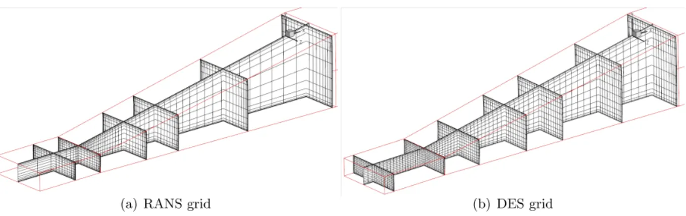
The computational domain is discretized with hexahedral cells. The grid distribution for the RANS simulations uses a two surface mesh distribution with a Hermite interpolation method to ensure orthogonal grids near the wall. The number of grid points is 296×41×61 along the
x,yand zcoordinates, a grid stretching of 1.2 was ensured near wall and ay+ ≈0.5. The grid
is also clustered along the streamwise direction towards the diffuser inlet as shown in 2.3(a). The grid resolution for the DES was determined by performing a study. Two grids are used as below,
the diffuser, while experiments indicate a separation skewed towards the doubly-sloped edge. The fine mesh predicts such a separation surface and hence was chosen for other simulations. The grid distribution is quite uniform as seen in Figure2.3(b) to maintain a cell aspect ratio close to unity.
The LES also are sensitive to grid resolution as noticed by Schneider et al. (2010). A grid of 3 Million cells is used (477×61×101) and quality checks are performed to assess the fidelity of simulations. LES quality metric tests are described in the next section. The grid is about 43 times smaller than the DNS grid used by Ohlsson et al. (2010). The near-wall mesh had a maximum of ∆y+= 2, ∆x+= 90 and ∆z+= 10. A large number of cells were required along
the streamwise direction, to generate a fully-developed flow at the diffuser inlet channel.
(a) RANS grid (b) DES grid
Figure 2.3 Mesh distribution in the diffuser showing every 4th node.
2.2.1 Codes and Numerics
Two codes were used for the RANS and eddy-resolving simulations. SuMB is used to perform the DES, while OpenFOAM is used for LES and RANS simulations. The turbulence model was implemented and validated in OpenFOAM.
2.2.1.1 SuMB
SuMB is a parallelized structured multi-block finite volume code (Van der Weide et al., 2006). Only a fully compressible solver is available, hence a preconditioner is required to apply it to low-Mach number flow. A few of the key parameter used for the solver are
• central with matrix dissipation for flux computations
• Roe’s Riemann solver with Van Albeda limiter
• 5-stage Runge Kutta smoother for flow variables and ADI smoother for turbulence quan-tities
• 3W multigrid
• Turbulence production term only considers strain
• Maximum ratio of TKE-production/dissipation: 1e5
• Fractional Time-stepping method allows for CFL>1
2.2.1.2 OpenFOAM
OpenFOAM is a parallelized unstructured finite volume code (www.openfoam.com). The incompressible solver is used with the following salient parameters:
• Conjugate gradient linear solver for pressure
• Bi-conjugate gradient solver for momentum
• The PISO algorithm is used with two corrector steps.
• To improve convergence, a limited central differencing is used for convective terms
• central difference for gradient and Laplacian terms
• second-order backward scheme is used for time derivatives.
• For RANS simulations, the SIMPLE method is used with Gauss-Seidel smoother for transport terms.
A channel with periodic inlet-outlet boundary condition was used. For DES the turbulence quantities are computed as,
ksgs= s 2 Cµ νsgs|S| ; ωsgs= k = p 2Cµ|S| (2.5)
from an LES of periodic channel. Using this a database of the fields U, V, W, ksgsandωsgs is stored in a 2-D plane, at equal intervals of time. This turbulence field is interpolated onto the inlet of DES based on the time step of the simulation. This method does not need a perturbed initial condition for the diffuser, as the inlet turbulence introduces that as flow iterations progress.
The LES did not require a precursor simulation, as OpenFOAM contains a feature to generate inflow for eddy resolving simulation. Data are mapped from a downstream plane upstream of the diffusing section to the inlet. Thereby, the initial section develops a fully-developed, turbulent profile. The mass flow through the mapping is fixed to the specified bulk flow. A random perturbation of the flow field is required to induce turbulence. Baba-Ahmadi and Tabor (2009) explain the flow mapping method. The length of the mapped domain is 10H as shown in Figure2.4.
Mapped Inlet
Figure 2.4 Flow domain with inlet mapping
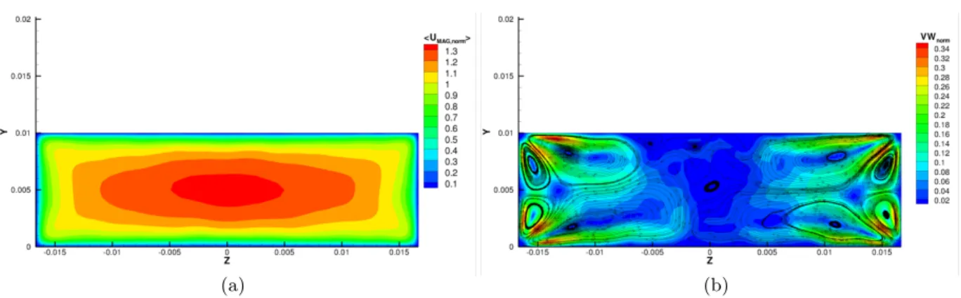
The fully-developed flow predicted by the LES is shown in Figure 2.5. It also shows the secondary flow caused by turbulence anisotropy. Though this secondary flow magnitude is about 5% of Ubulk, it affects the separation structure.
(a) (b)
Figure 2.5 Primary and Secondary velocity profile in the fully-developed rectangular channel of A=3.33. Statistics were averaged over 50 flow-through times.
2.2.3 Computing resources
All the simulations were performed in parallel on Linux SMP clusters. The MPICH standard is used for data transfer across compute nodes by both codes. SUMB required the number of grid nodes along each coordinate direction to be a multiple of 4 for 3-level Multigrid to be used. The DES was converged at every time level with 80 pseudo-time iterations, a large time step (10 times larger than LES) was possible, as the numerical time integration method was not limited by CFL criteria. The LES is most expensive as seen in Table 2.2, due to stringent near-wall grid requirement. Moreover, statistical averaging was required over a large flow-through times T U∞
L
to converge the high-frequency fluctuations, increasing the simulation time. Table 2.2 summarizes the typical compute resources for each simulation. The RANS compute times for both solvers were quite comparable. The EARSM simulations were initialized using SST-predicted flow field and simulated for 400 CPU hours to convergence level.
Simulation Grid size (×106 cells) CPU’s Wall time CPU Hours
LES 3 128 27 days 83,944
DES 1.8 128 3.5 days 10,752
RANS – SUMB 1.2 64 17 hours 1,088
RANS – OpenFOAM 1 32 23 hours 736
CHAPTER 3. EDDY-RESOLVING SIMULATIONS
Separation being a highly unsteady phenomena, time-resolved simulations of the flow field were required to resolve the turbulent structures and the energy cascade. The LES and DES simulation methods described in this chapter are collectively referred to as ‘eddy-resolving’. This nomenclature is primarily to distinguish them from the RANS computations.
3.1 Detached Eddy Simulations
While LES is capable of resolving eddies and the turbulence spectrum, it requires a large number of grid points in the near wall region. Most of the near wall structures need to be resolved in order to compute the turbulent boundary layers. DES is a hybrid LES/RANS model, introduced to alleviate the near-wall grid requirement. The boundary layer region is solved with RANS and the separated region with eddy simulation. The basic DES model switches from RANS to eddy simulation automatically, based on the distance to wall and local grid spacing. However there is an issue: if the near wall mesh is too fine, the RANS model can switch off. This was address by the Scale Adaptive Simulation (SAS) method of Menter et al. (2003). Here the length scale is dependent on the local flow variables, rather than on grid spacing. This allows the eddy resolved region to change dynamically, while preserving RANS near the wall. The length scale parameter used is
Lνk =κ ∂U/∂y ∂2U/∂y2
The k-ωShear Stress Transport (SST) model of Menter (1994) is used in the RANS region. With the stress limiter, this RANS model has proved to predict 2-D separation accurately in a variety of APG boundary layer flows. A fine near wall mesh (y+ ≈ 0.6) allows the RANS
Due to the low Reynolds number of the channel flow, well resolved simulations could be made with small sub-grid viscosity. The spectral resolution of the simulation is assessed by probing the time-varying streamwise velocity in the bulk flow and analyzing the power spectral density. From Figure 3.1 we notice 3 orders of frequency resolved, with the inertial range following the -5/3 slope. The energetic spectral range widens and increases in magnitude as the flow moves downstream. No periodic frequency is seen. Hence, the flow is statistically stationary and Reynolds averaging is synonymous with time averaging.
(a) Probe 1, x/H=3 (b) Probe 2, x/H=6
(c) Probe 3, x/H=9 (d) Probe 4, x/H=12
Figure 3.1 Power spectrum of instantaneous streamwise velocity. The 4 probe points are located at the centroid of cross-sectional planes that are equally spaced from inlet to outlet. The -5/3 slope line is in red.
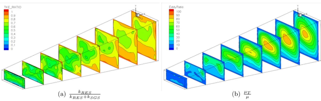
The resolution of the turbulent energy is shown in Figure3.2. The ratio of the resolved-to-total turbulent kinetic energy indicates that more than 50% of the energy is resolved. The eddy viscosity ratio is lower than 50 in the bulk of domain, except at the core of flow downstream where the mesh size is largest. These checks ensure the quality of DES results.
(a) kRES
kRES+kSGS (b)
µT
µ
Figure 3.2 The ratio of the resolved-to-modeled turbulent energy in the baseline diffuser DES.
3.1.1 Validation
The Cherry et al. (2008) Diffuser 1 has been simulated and compared to experiments. This case will hereafter be referred as the baseline diffuser. The mean flow is calculated by averaging the flow over 10 flow-through (τ) times, with the averaging starting after 8τ. The streamwise velocities at transverse planes show a decent agreement with experiments (Figure 3.3). DES results shows a separation in the top left corner, which is absent in experimental data. The simulations predict the correct topology of separation on the top wall of the baseline case, though the volume of reverse flow is over-predicted. Too large reverse flow has also been predicted by hybrid LES-RANS simulations of Abe and Ohtsuka (2010) and SAS of Uribe et al. (2010). A detailed plot of the velocity at streamwise and spanwise locations is shown in Figure 3.4. The DES predictions indicate a higher velocity gradient close to the wall, which causes the pressure at the wall to be low, thus the pressure recovery in the diffuser is less than the experiment.
In contrast, the SST model predictions are qualitatively incorrect, separating on the wrong wall of the diffuser (Fig. 3.4). The secondary flow predictions did not agree with experiments either, but, as the secondary flow magnitudes are quite low (≈%10Ubulk), their measurement accuracy are questionable.
2 cm 5 cm 8 cm 12 cm 15 cm
Figure 3.3 Streamwise velocity predicted using SAS and experimental measurements of Cherry et al. (2006) at transverse planes. Contour lines are spaced 0.1 m/s apart. The zero-streamwise-velocity contour line is thicker than the others.
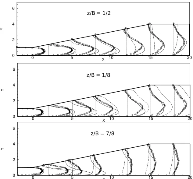
X Y 0 5 10 15 20 0 2 4 6 X Y 0 5 10 15 20 0 2 4 6 X Y 0 5 10 15 20 0 2 4 6 z/B = 1/2 z/B = 7/8 z/B = 1/8
Figure 3.4 Variation of mean streamwise velocity along spanwise z-lines. B is the width of the diffuser at that x-location. The solid lines are DES, and dashed k−ω SST model compared with experimental data.
3.1.2 Study of flow separation
The computed DES results predict the correct separation topology and decent quantitative match with experiments. The wall-limiting streamlines on the baseline diffuser indicate where the flow separates from the wall. A number of nodal points are seen in Figure3.5on the sloped walls. Vortices originate from these singular points and convect through the boundary layer and reverse flow region. A clockwise vortex originates from a focus on the top wall and convects towards the side wall.
(a) (b)
Figure 3.5 Secondary flow in baseline diffuser predicted by DES. (a) The wall limiting stream-lines indicate the separation structure. (b) secondary flow at transverse planes having streamwise vortices, the separation line is in red.
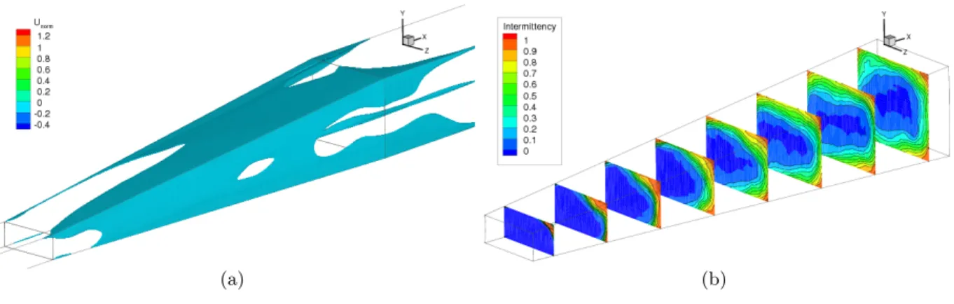
All of the two-equation RANS models predicted a transition of separation from top to side walls at aboutA2.5. A DES of the series of diffusers is analyzed to know the efficacy of RANS models. These simulations indicated the averaged flow separation to be on the side wall for both A2 and A2.5. The results of A2.5 are interesting as the flow is highly unsteady. In order that flow averaging be a meaningful way of analyzing the flow field, the unsteadiness has to be quantified. The flow intermittency is measured as the ratio of times the flow reverses to that of the streamwise direction. In Figure3.6, the flow is unidirectionally streamwise towards the core of the diffuser, however values of 1 are observed towards the sloped corner and sides, indicating reverse flow to always exist there. Hence though the separation surface indicates partial separation on top, the separation is considered to be on the side wall. Movies of time-evolution of the separation surface show the separation surface to be attached to the side wall
exists a counter-clockwise churning, which convects flow from side to the top wall causing the separation surface (U ≡0) to be unsteady.
(a) (b)
Figure 3.6 Separation bubble(a) and Intermittency(b) in the A2.5 diffuser predicted using the DES model.
(a)A2 (b)A2.5
Figure 3.7 Secondary flow show a similarity in pattern at different inlet aspect ratios. The foci is formed earlier in the A2.5 diffuser and moves downstream
3.1.3 Vortical flow features
While the secondary flow magnitudes are only about 5% of the bulk velocity, they provide critical insight into the dynamics of the flow. The flow contains streamwise vortices that interact downstream the diffuser. Resolving these vortices are a challenge to existing RANS models,
as they dissipate faster and also overpredict turbulence production at the vortex core. The limiting streamlines in Figure3.8identify the various singular points on the diffuser surface as foci and saddle nodes. The identification and classification of these nodes is made by a visual comparison of the nature of the streamlines at these critical points (D´elery, 2001). The theory behind classifying these points is described in the previous reference, which could be used in automated classification of these points. The foci are identified by coiled streamlines that converge at the core where τl(l, m) =τm(l, m) = 0, where l and m are wall coordinates. The saddle nodes appear where streamlines converge or diverge by bending 90 deg. In A2.5 there are 3 foci and one saddle node, the separation surfaces emanate from where the wall streamlines converge and flow attachment at locations where streamlines diverge. The wall shear stress is non-zero at separation/attachment surfaces, as there exists cross-flow along these surfaces. From each of the focus vortices originate as shown in Figure3.8 and interact downstream.
(a)
(b)
Figure 3.8 (a)Limiting streamlines for A2.5 diffuser on the wall show a steady separation surface from the top wall, The side wall has a complex separation-attachment flow. (b)The vortex cores show a vortex originating from foci F3 on left and multiple vortices close to the double-sloped edge
The limiting steamlines on the diffuser cases A2 and A2.5 are identical, but the corre-sponding secondary flow inside the diffuser develops quite differently. Hence vortex interactions critically differentiate the flow in the series. ForA2.5, the wall streamlines have the singular points closer to the diffuser inlet than in A2 (Jeyapaul and Durbin, 2010), hence there is more room for the vortices originating from them to develop along the APG boundary layer
the corner subjected to the APG. As the flow develops downstream, two vortices (at x/H=4) are introduced from the foci F1 and F2. These vortices interact and unify creating one vortex at x/H=5.8, this disintegrated downstream creating multiple vortex foci and a saddle node.
(a) x/H=1 (b) x/H=4
(c) x/H=5.8 (d) x/H=13.7
Figure 3.9 Secondary flow streamlines in transverse planes of A2 diffuser. The blue line indicates the location of separation surface.
3.2 Large Eddy Simulations
LES are widely used to predict complex shear flows. The simulations were performed using the dynamic Smagorinsky model, in the incompressible solver of OpenFOAM. A test filter is performed on a larger size than the grid filter. The resolved Reynolds stresses in this ‘test window’ is representative of the sub-grid stresses and is used to evaluateCslocally. Due to this, the model does not need near-wall damping. The effective SGS viscosity(ν+νt) is set to zero in regions where the value becomes negative. The sub-grid stress is modeled by expression3.1,
where sub-grid viscosity is given byνt= (Cs∆2)|S|, which is a linear eddy-viscosity assumption. τij − 1 3τkkδij =−2(Cs∆) 2|S|S ij; where|S| ≡ p 2SijSij (3.1)
Since filtered Navier-Stokes equations change for different grid resolutions, the way to check the accuracy of the simulation is to compare the resolved first and second moments of the primitive flow variables. Celik et al. (2009) has a list of assessment measures to ensure the quality of LES. Errors in LES have the following sources: modeling, numerical and filtering. In order to isolate the modeling and discretization errors, a minimum of two to three grid calculations are necessary (Celik et al., 2009). In the interest of computational time, only a single grid case was used to check for LES errors. From the grid refinement studies with DES, the LES grid was arrived at with a refined near-wall grid with a cell expansion ratio of 1.05. The grid used for the simulation has 3 Million cells.
Single grid estimator checks were performed on this grid for the baseline diffuser. The spectrum of turbulence resolved by LES is indicated by a Fast Fourier analysis of data at point probes located along the bulk of the flow. The data were collected over 75 flow though times; the time required to converge mean flow statistics is shown in Figure 3.10. The frequency resolved spectrum is five orders of magnitude wide, as compared to 3 orders by the DES. We notice the inertial range to contain eddies whose energies cover by 3 orders of magnitude. The slope of this range does not follow Kolmogorov’s scaling of -5/3. The reason for this higher slope is due to the low Reynolds number of the diffuser and also the non-homogeneity of the flow. The grid size used has a filter cut-off frequency of about 3×10⁴Hz, which is the location where the spectrum changes slope. As this low energy region is relatively short, the error introduced due to sub-grid models is small.
The accuracy of the simulations was verified by a quantitative check on the amount of turbulent energy resolved:
kres
ktot
= kres
kres+ksgs+|knum|
To evaluate the numerical error in the simulation, an LES on a different grid size would be required; in our check, the numerical error was neglected. About 95% of the turbulent kinetic
(a) Probe 1, x/H=3 (b) Probe 2, x/H=6
(c) Probe 3, x/H=9 (d) Probe 4, x/H=12
Figure 3.10 Power spectrum of instantaneous streamwise velocity predicted by LES. The 4 probe points are located at the centroid of cross-sectional planes that are equally spaced from inlet to outlet. The -5/3 slope line is in red.
energy is resolved (Figure3.11), hence the flow is close to DNS resolution. Celik et al. (2009) suggested the calculation of arelative sgs-viscosity index as;
LES IQν = 1 1 +αν ν ef f ν n
where,νef f =νsgs+νnum+νandαν = 0.05, n=0.53. This quantity is the ratio of eddy-viscosity and is close to 1 in the flow, which, hence, is well resolved.
(a) (b)
Figure 3.11 The quality of the LES assessed using the metric of (a) Ratio of resolved to total Turbulent kinetic energy and (b)LES IQν parameter
While the overall quality of the flow was assessed to be of good quality, a validation exercise is required for the flow variables predicted using this simulation.
3.2.1 Verification
The numerical stability of the LES was ensured by maintaining a CFL number less that 1, which required a time step of ∆t∼10−5s. The flow is initialized by random fluctuations and is allowed to develop for about 27τave (flow throughs based on average bulk velocity in diffuser). The averaging is later started and continued for 70τave, which was required to converge the mean and second-moments of flow velocity. The actual averaging required differed from diffuser-to-diffuser. Notably, Diffuser 2 of Cherry et al. (2008) required about 100τave to converge the statistics.
With the availability of DNS data of Ohlsson et al. (2010) a more detailed comparison of flow variables has been made. The mean streamwise velocity and the dominant Reynolds stress
of separation is also under predicted. The results presented here use a sharp-edged diffuser inlet, while the DNS used a filleted edge. A bulk of the turbulent kinetic energy comes from the streamwise normal stress uu, and the values compare quite well. A high normal stress is predicted at the sloped edges at inlet, than by DNS this is caused due to the high shear introduced by the sharp edge. Downstream of the diffuser, the magnitudes and trends of uu
agree well. 0 0 0 0 0 .1 0.1 0 .1 0.1 0.2 0.2 0.2 0.2 0.3 0.3 0.3 0 .4 0.4 0.4 0 .4 0 .5 0.5 0.5 0.6 0.6 0.6 0.7 0.7 0.8 0.8 0.9 0.9 1 0 0.1 0.1 0.1 0.2 0.2 0.2 0.3 0.3 0.3 0.4 0.4 0.4 0.5 0.5 0.5 0.6 0.6 0.7 0.7 0.8 0.8 0.9 0.9 1 0 0 0 0 0 0.1 0 .1 0.1 0.1 0.2 0 .2 0.2 0 .2 0.3 0.3 0.3 0.4 0.4 0.4 0.5 0.5 0.5 0.6 0.6 0 .7 0.7 0.8 0.8 0.9 0 .1 0.1 0 .1 0.1 0.2 0.2 0.2 0.3 0.3 0.3 0 .4 0.4 0.4 0.5 0.5 0.6 0.6 0.7 0 .7 0.8 0.9 0 0 0 0 0.1 0.1 0.1 0 .1 0 .2 0.2 0.2 0 .2 0.3 0 .3 0.3 0 .4 0.4 0.4 0.5 0.5 0 .6 0.7 0.8 0 .1 0.1 0 .1 0.2 0.2 0.3 0 .3 0.4 0 .4 0.6 0.5 0 .7 0 0 0 0 0 .1 0 .1 0.1 0 .1 0.2 0.2 0 .2 0 .3 0 .3 0.3 0.4 0.4 0.5 0.6 0.7 0 0 .1 0 .1 0.2 0.2 0.3 0 .3 0.4 0.5 0.6 -0.1 0 0 0 00 .1 0.1 0.1 0.2 0.2 0.3 0.3 0.4 0.5 0 0.1 0.1 0.2 0 .2 0.3 0 .3 0.4 0.5 2 5 8 12 15 x/H
(a)u/ubulk
urms 20 18 16 14 12 10 8 6 4 2 2 5 8 12 15 x/H (b) 100urms/ubulk
Figure 3.12 Contour lines of mean streamwise velocity and streamwise RMS velocity at various transverse planes. The DNS is to the left and LES on the right on each of Figures (a) and (b). Each line is spaced by 0.1 and the zero velocity line is bold.
3.13compares the mean flow velocities and normal and shear stress quantities in the mid-plane of the diffuser with DNS. Comparisons at other z-planes close to the asymmetric wall and the parallel wall showed a similar good agreement, and are shown in Figures3.14-3.16. The spike in all the Reynolds stress is observed close to the diffuser inlet. This is only a local effect due to the geometric difference and the flow develops downstream, giving a better comparison to DNS. Near the bottom wall the velocity gradients are steep and have been captured by the dynamic LES model. Resolving this gradient is critical to predicting the wall pressure coefficientCp accurately. At the inlet to the diffuser, theuiuj profile is similar to that of a fully developed flow in a 2-D channel, with the uv changing signs at mid-channel. The effect of the 3-D separation deviates the flow from turbulence equilibrium causing the maximum Reynolds stress to exist close to the centre of channel. In the straight section downstream of diffuser, the flow does not show signs of relaxing to equilibrium from the mean velocity and stress profiles.
velocity at that location. Good agreement with experiments is shown in Figure3.17. The wall pressure follows the effects of separation manifesting as blocked cross-sectional flow area. Data show a rapid rise in Cp near the inlet of the diffuser, followed by a gradual reduction in the pressure gradient until the trend becomes nearly linear at about x/L=0.7. At this point, the reverse flow region has spread almost uniformly across the top expanding wall. The pressure profile contains an inflection point at about x/L=0.4, where separation is still at the sloped corner. The pressure curve shows no change of slope at x/L=0.53, the position where the separation bubble leaps across the top expanding wall of the baseline diffuser. Near the inlet, the flow area expands rapidly and the separation bubble is small, resulting in a large expansion of the potential flow area, hence a large pressure gradient. Farther downstream (0.2 <x/L <
1), the separated region grows rapidly and somewhat counteracts the growing cross-sectional area of the diffuser by reducing area for forward flow. This results in a more gentle pressure gradient. Downstream fo the diffuser outlet (x/L>1) the flow reattaches recovering additional pressure.
3.2.2 Diffuser series
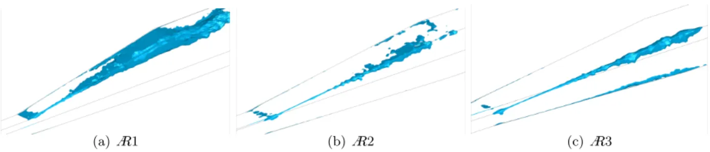
The series of diffusers simulated using LES show separation to switch to the side wall at about A3. As noticed in Figure 3.18 the volume of separated flow reduces as Aincreases, which improves the efficiency of the diffuser as the wall pressure recovery reaches a maximum of 80% for A> 2. The secondary flow are similar, each case having 4 major vortices located at diffuser exit(x/H=15) transverse section. Figure 3.19 shows the vortex cores to be located away from the reverse flow region, but towards the corners. In a sense, the major streamwise vortices are displaced by the reverse flow region.
0 0.5 1 1.5 2 2.5 3 3.5 4 0 5 10 15 20 25 (a) U 0 0.5 1 1.5 2 2.5 3 3.5 4 0 5 10 15 20 25 (b) V 0 0.5 1 1.5 2 2.5 3 3.5 4 0 5 10 15 20 25 (c)uu 0 0.5 1 1.5 2 2.5 3 3.5 4 0 5 10 15 20 25 (d) vv 0 0.5 1 1.5 2 2.5 3 3.5 4 0 5 10 15 20 (e) uv 0 0.5 1 1.5 2 2.5 3 3.5 4 0 5 10 15 20 25 (f) uw
Figure 3.13 Comparison of mean flow velocities, resolved kinetic energy, and Reynolds stresses along z/B=1/2by LES of baseline diffuser. DNS are solid and LES are dashed.
0 0.5 0 5 10 15 20 25 (a) U 0 0.5 1 1.5 2 2.5 3 3.5 4 0 5 10 15 20 25 (b) W 0 0.5 1 1.5 2 2.5 3 3.5 4 0 5 10 15 20 25 (c)uu 0 0.5 1 1.5 2 2.5 3 3.5 4 0 5 10 15 20 25 (d) vv 0 0.5 1 1.5 2 2.5 3 3.5 4 0 5 10 15 20 (e) uv 0 0.5 1 1.5 2 2.5 3 3.5 4 0 5 10 15 20 25 (f) uw
Figure 3.14 Comparison of mean flow velocities, resolved kinetic energy, and Reynolds stresses along z/B=1/4by LES of baseline diffuser. DNS are solid and LES are dashed.
0 0.5 1 1.5 2 2.5 3 3.5 4 0 5 10 15 20 25 (a) U 0 0.5 1 1.5 2 2.5 3 3.5 4 0 5 10 15 20 25 (b) W 0 0.5 1 1.5 2 2.5 3 3.5 4 0 5 10 15 20 25 (c)uu 0 0.5 1 1.5 2 2.5 3 3.5 4 0 5 10 15 20 25 (d) vv 0 0.5 1 1.5 2 2.5 3 3.5 4 0 5 10 15 20 (e) uv 0 0.5 1 1.5 2 2.5 3 3.5 4 0 5 10 15 20 25 (f) uw
Figure 3.15 Comparison of mean flow velocities, resolved kinetic energy, and Reynolds stresses along z/B=3/4by LES of baseline diffuser. DNS are solid and LES are dashed.
0 0.5 0 5 10 15 20 25 (a) U 0 0.5 1 1.5 2 2.5 3 3.5 4 0 5 10 15 20 25 (b) W 0 0.5 1 1.5 2 2.5 3 3.5 4 0 5 10 15 20 25 (c)uu 0 0.5 1 1.5 2 2.5 3 3.5 4 0 5 10 15 20 25 (d) vv 0 0.5 1 1.5 2 2.5 3 3.5 4 0 5 10 15 20 (e) uv 0 0.5 1 1.5 2 2.5 3 3.5 4 0 5 10 15 20 25 (f) uw
Figure 3.16 Comparison of mean flow velocities, resolved kinetic energy, and Reynolds stresses along z/B=7/8by LES of baseline diffuser. DNS are solid and LES are dashed.
x/L Cp 0 0.5 1 1.5 0 0.1 0.2 0.3 0.4 0.5 0.6 Expt SST LES-dynSmag
Figure 3.17 Coefficient of pressure Cp = p −pref 0.5ρU2 bulk
variation along the bottom wall of base-line diffuser predicted by LES, x/L is the non-dimensional diffuser length. The experimental Cp has been shifted by -0.02 to provide a better comparison.
(a)A1 (b)A2 (c)A3
Figure 3.18 Separation surface predicted by LES for the diffuser series
3.3 Comparison of LES and DES
The motivation for using the DES was due to the reduced grid requirement than an LES. The former provided a qualitative comparison with experiments, however a good quantitative comparison is paramount to generate data needed for turbulence model development. The SAS predicts a larger separation (Figure3.20) than LES and separation spreads over the whole top wall ahead of the streamwise location shown in experiments. The wallCp predictions are much lower due to the higher flow blockage. Similar observations of lowCp and larger separation are observed by SAS simulations of Uribe et al. (2010) and hybrid LES-RANS of Abe and Ohtsuka
(a)A1 (b) A2 (c)A3
Figure 3.19 Secondary flow predicted by LES at the diffuser exit plane x/H=15 of the diffuser series. The cross-sections are shown in different scale, in real the areas are same.
(2010). The main reason for the inaccuracy of the DES arises from the inability of the near wall RANS, k−ω SST model in the SAS to predict Reynolds stress anisotropy that occur in the corner flow of diffuser. This will be the subject of discussion in the next chapter.
The LES have been computationally intensive both in grid requirement and numerical solution, however the flow predict compare well with DNS. The Reynolds stress budget terms (Pij, ij,Πij, Dij) are accurate and can be used for model development.
Figure 3.20 Fraction of cross-sectional area separated predicted by DES and Experiments for the baseline diffuser
CHAPTER 4. SINGLE POINT CLOSURE MODELS
Turbulence modeling has been focused on single-point correlations for their tractability. The cost of this assumption is that the whole spectrum of turbulence scales cannot be resolved as possible by multi-point correlations. Statistical approach as Reynolds averaging is required to simplify the analysis of Navier-Stokes equations, as given by the RANS equations in (4.1). The mean is represented as U =U and fluctuation u= 0.
∂tUi+Uj∂jUi=− 1 ρ∂iP+ν∇ 2U i−∂jujui (4.1) ∂iUi= 0
The Reynolds stress tensor (bold in 4.1) is unknown and needs the solution of second-moment transport equations. Higher (n+1) moment terms occur in a n-moment equation, which lead to the closure problem. Most engineering turbulence models solve for first-moment equations(4.1) with a model for the stress term. The Boussinesq assumption is widely used to close the RANS equation. −uiuj = 2νTSij− 2 3kδij (4.2) In two-equation models,νT =Cµk 2 = k
ω the former for the k−model and the later fork−ω model. The algebraic expression in 4.2 has been successful in predicting a variety of flows. However in complex flows with separation, streamline curvature, frame rotation, stagnating flows, etc the Boussinesq assumption fails.
4.1 Linear eddy-viscosity models (LEVM)
A linear relation between Turbulent stress and mean-flow strain limits the ability to model few flow effects. The stress anisotropy is defined as aij = uikuj −23δij, where k= 12uiui. Hence
one can analyse the departures from isotopy (aij = 0) by looking at the 5 distinct elements of this symmetric and trace-free matrix. In the eddy viscosity models the anisotropy is a function of strain only,aij =−2νTSij. Due to this assumption the following are the drawbacks:
• Normal stress anisotropy is not accounted.
• Only accurate for equilibrium flows
• No streamline curvature effects included, asaij =Fij(Sij)
As mentioned earlier, secondary normal stress anisotropy (v26=w2) is required to predicting
secondary flow of second-kind. At the vicinity of stagnation point, the primary-secondary stress anisotropy (u2 6=v2) needs to be resolved to predict the correct turbulence production and hence
kinetic energy. This was corrected by limiter on the turbulence timescale by Durbin (1996). The model coefficients are most determined from idealized flow conditions, such as homo-geneous shear and plane shear flow. The deviation of the flow from turbulence equilibrium is measured by the ratio of Production-to-dissipation P/ε. Where;
Pij =−uiuk ∂Uj ∂xk −ujuk ∂Ui ∂xk ; εij = 2 3εδij =⇒ P ε =−uluk ∂Ul ∂xk 1 ε =−aij Sijk ε
In plane shear flow P/ε = −a12dyU(k/ε) and hence the accuracy of predicting the ratio is only dependent on modeling fidelity of Reynolds shear stress. Most models are calibrated based on this flow −kuv = p
Cµ(= 0.3). In two-dimensional APG and separated flows, this fails, leading to over prediction of eddy-viscosity. Menter (1994) introduced a stress limiter redefiningνT.
4.1.1 Anomalies in predicting 3-D separation
Three-dimensional separation is nearly independent of the Reynolds number and is char-acterized by two adjacent boundary layers subjected to APG. The modeling challenges are rooted in the complexity of the strain and vorticity field. To predict separation in asymmetric diffusers the model has to resolve the complex 3-D flow, lateral straining, stramline curvature, streamwise vorticity, secondary flow of second kind, and effect of transverse pressure gradient.
are shown in Figure4.1. The primary flow is formed initially along the top, but later switches to the side sloped wall. The flow predicted at the first section in4.1(b) compares well with the SAS, both the primary and secondary flow with vortices and singular points. However down-stream SST predicts the vortices to dissipate faster and separation is formed on the wrong wall. A similar primary flow separation is predicted by the tested LEVM. The v2−f predicts the
near-wall anisotropy accurately, however fails to predict the separation on the top wall, due to the three-dimensional nature of the flow separation. A modified implementation of this model, theζ−f was tested by Ryon (2008) to produce the same error.
(a) (b)
Figure 4.1 Primary and secondary flow predicted using thek−ω SST model. The transverse velocity in (b) is normalized by Ubulk
Flow separation in the diffuser series predicted by SST indicate a switching of separation from top to side wall at aboutA2. However eddy-resolving simulations predict the switch to happen at A2.5. The SST model responds to the increase in Amuch faster than LES, thus are oversensitive to minor transverse pressure. Qualitatively a correct separation is predicted by RANS for the rest of Aseries, but the separation volume is high and hence streamwise velocities increase leading to a lower wall pressure coefficient predicted than by the LES.
In diffuser configurations, the SST model showed sensitivity to minor changes in geometry. Few are;
(a)A1 (b)A1.5
(c)A2 (d)A2.5
Figure 4.2 Separation surface predicted by SST model in the series of diffusers.
Side slope angle asymmetry
On the diffuser with sloping on one of the transverse direction only, the model predicts separation on the sloped top wall. However even with an infinitesimal slope (0.02 deg), the separation surface moves to the small-sloped side. This diffuser has the same A=3.33 of the baseline. The physics of flow predicted by SAS shows the separation on the top wall. In the top-only sloped geometry the area expansion increases linearly with x, and so is the streamwise pressure gradient. However the introduction of secondary slope make the area expansion rate with x quadratic and dp/dx follows the trend. This corroborates with the earlier observation that the SST model is highly sensitive to transverse pressure gradients.
Higher symmetric side slope
A series of diffusers with a constant top slope and inlet Ais created, the side walls are flared symmetrically with different angles. As the side slope angles increase, the dp/dx gets
was initialized, in a sense bistable.
(a) 1 deg (b) 2.56 deg
Figure 4.3 Anomalous separation surface predicted by SST in diffusers with symmetric side slope angles.
Flow predicting by DES did not indicate an asymmetric flow at 2.56 deg, but a total sepa-ration on the top wall. The Reynolds stress model of SSG showed a similar sepasepa-ration, but of smaller reverse flow. The Spalart-Allmaras model predicted a symmetric side wall separation at all angles. Hence there is a disparity in predictions among RANS models for this series, how-ever incorrect. The SST model destabilize in predicting separation at high streamwise pressure gradients.
4.2 Sensitizing Cµ to flow separation
The Cµ = 0.09 is calibrated for 2-D mild shear flows. Hence sensitizing the coefficient to general 3-D shear flows would make the model accurate to predict flow separation. The effect of increasingCµin the standardk−ωSST model causes separation to decrease in the Obi et al. (1993) diffuser (Figure4.4). The increase in the coefficient’s value leads to a direct increase in eddy-viscosity which causes more dissipation and hence a smaller separation. As complex flows are composed of a variety of fundamental flow physics, havingCµ change locally based on the flow velocity would be required to resolve the local flow. Some of the modeling parameters are