Pattern Recognition Using K-Nearest Neighbors (KNN) Technique

(1)

PATTERN RECOGNITION USING K-NEAREST NEIGHBORS (KNN) TECHNIQUE

By

MOHD FARISFAIZ BIN CHE LAH

FINAL PROJECT REPORT

Submitted to the Electrical & Electronics Engineering Programme in Partial Fulfillment of the Requirements

for the Degree

Bachelor of Engineering (Hons) (Electrical & Electronics Engineering)

Universiti Teknologi Petronas Bandar Seri Iskandar 31750 Tronoh

Perak Darul Ridzuan

(2)

CERTIFICATION OF APPROVAL

Pattern Recognition Using K-Nearest Neighbors (KNN) Technique

by

Mohd Farisfaiz Bin Che Lah A project dissertation submitted to the Electrical & Electronics Engineering Programme

Universiti Teknologi PETRONAS in partial fulfillment of the requirement for the

BACHELOR OF ENGINEERING (Hons) (ELECTRICAL & ELECTRONICS ENGINEERING)

Approved by,

_____________________ (Dr Brahim Belhaouari Samir) Project Supervisor

UNIVERSITI TEKNOLOGI PETRONAS TRONOH, PERAK

(3)

CERTIFICATION OF ORIGINALITY

This is to certify that I am responsible for the work submitted in this project, that the original work is my own except as specified in the references and acknowledgements, and that the original work contained herein have not been undertaken or done by unspecified sources or persons.

___________________________________________ MOHD FARISFAIZ BIN CHE LAH

(4)

ABSTRACT

The aim of this project is to develop a better image processing algorithm using K-Nearest Neighbors (KNN) technique. This project will apply supervised learning, thus require the author to gather training data and testing data consist of written alphabets. The algorithm will be built in the Matlab. Initially, the author needs to introduce the simpler version of feature extraction to replace the present extractor that more complex and time consuming. The basic idea of this type of feature extraction is to apply various shapes of curls on an image and the intersection of these two produce a stream vector. This step will be applied for entire images. For classification phase, there are two type of classifier that will be used which are Traditional K-Nearest Neighbors(KNN) and Clustering K-Nearest Neighbors(C-KNN).The result of each classifier will be analyze to get the optimal result or accuracy. Next, sample data need to be added in order to measure the robustness of algorithm. For the future, it is recommended that another version of input applied to the algorithm such as signature and thumbprint. If possible, the author also needs to build the hardware or application module that able to perform an accurate recognition and user-friendly.

(5)

ACKNOWLEDGEMENT

First of all, I would like to express my greatest praise to Allah S.W.T after successfully finish my final year prject. With my sicere appreciation, I would like to give my utmost gratitude to my supervisor, Dr Brahim Belhaouari Samir for his detailed and constructive comments along with continuous assistance, support and motivation from beginning until the end of the project

My most appreciation also goes to him especially for the entire efforts and contribution of his ideas also guidance in Matlab programming. His expertise and wide knowledge have been great value for me.

Above all, I thank my family for always standing there besides me and continuously supportive throughout my life.

Last but not least, my regards and blessing also goes to all lecturers and colleagues who had supported me in any aspect while completing this project.

(6)

LIST OF FIGURES

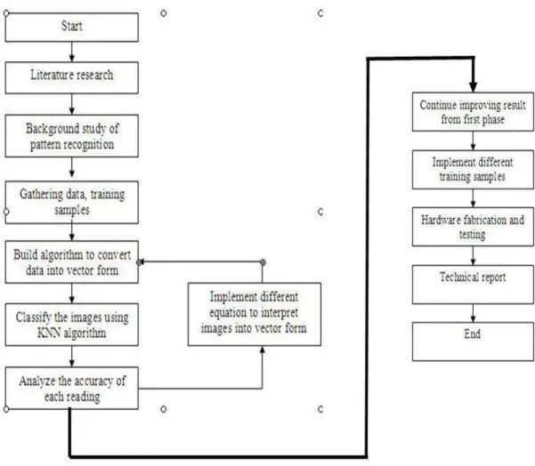
Figure 1: Spiral Equation to Interpret Image . . . 5 Figure 2: Classification Using KNN Technique of Three Different Features 7 Figure 3: Classification Using Improved KNN/Cluster KNN . 8 Figure 4: Progress Flow for the Whole Project . . . . 9

Figure 5: Training Samples . . . 10

Figure 6: Image Enhancement Using Morphological Operation . . 11 Figure 7: Algorithm to Extract the Features and convert the Data into Vector Form 12 Figure 8: Algorithm To Classify The Image Using KNN Method . . 14 Figure 9: K-Means Clustering Algorithm . . . 16 Figure 10: Feature Extraction Using Logarithmic Spiral before Parameter Tuning 19 Figure 11: Feature Extraction Using Logarithmic Spiral after Parameter Tuning 19 Figure 12: Comparison between Feature Extraction Using Fermat/Logarithmic 20 Figure 13: Initial Curl for Galaxy . . . 21 Figure 14: Angled-Shifted Curl for Galaxy . . . 21 Figure 15: Feature Extraction of Images Using Galaxy Equation . . 22 Figure 16: Comparison between Unidirectional Galaxy with Bidirectional Galaxy 23 Figure 17: Graph of Average Accuracy For Each Methods . . . 28 Figure 18: Analysis on Accuracy When Varying K Value . . . 29 Figure 19: Graphical User Interface . . . 30 Figure 20: Proposed Module for Signature Recognition System . . 31

(9)

LIST OF TABLES

Table 1: List of Hardware and Software Used in This Project . . 17 Table 2: Result of Accuracy after Parameter Tuning for Logarithmic Spiral 24 Table 3: Result of Accuracy after Parameter Tuning for Multiple Spiral . 25 Table 4:Result of Accuracy after Parameter Tuning for unidirectional Galaxy

Equation . . . 26

Table 5: Result of Accuracy after Parameter Tuning for bidirectional Galaxy

Equation . . . 27

Table 6: Average Accuracy Produced By Each Method for KNN and C-KNN 28 Table 7: Effect on Accuracy While Varying K Values . . . 29

(10)

CHAPTER 1 INTRODUCTION

1.1Background of Study

Pattern recognition is the process of interpreting raw data and taking an action based on the category of the pattern [4]. Description scheme is usually based on the availability of a set of patterns that already have been classified. This patterns called training set and this method can be categorize as supervised learning. Meanwhile, in unsupervised learning, system is not given an exact labeling of the patterns instead it establishes the classes based on statistical regularities of the pattern. [4]Regression and classification methods based on similarity of the input have been widely used in applications which involve large set of high-dimensional data.[1] One of the most preferable methods in cluster analysis is k-means clustering. The algorithm will use K-nearest neighbors (KNN) technique to classify each training samples into their respective cluster.

(11)

1.2Problem Statement

Many researchers have found that the KNN algorithm accomplishes very good performance in their experiments on different data sets. The traditional KNN text classification algorithm has three limitations which are calculation complexity, dependence on training set and no weight difference between samples. [9]. Besides, the current system of recognition, normally use Neural Network and Wavelet Transform to extract the feature from image. The author found that these approaches are more complex and time consuming. Hence, the author will attempt new approach in extracting the features which more simple and resulting in non-lengthy vectors to reduce the execution time. In addition, the existing systems also consume high cost to be implemented and too complicated to be handled by the user. Therefore, the author will try to come out with a system with a reasonable cost and less complexity

1.3Objectives

The objectives of this project are:

 To implement K-Nearest Neighbors(KNN) algorithm in classifying sample data into their respective cluster

 To introduce the new approach in extracting features from image

 To come out with an accurate recognition system which using K-Nearest Neighbors(KNN) methods

(12)

1.4Scope of Study

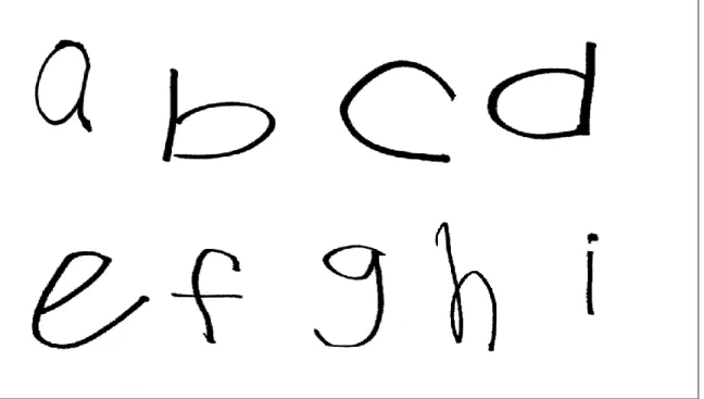
During early phase of this project, literature research has to be made in order to gather the information about the current classifier system and their weaknesses. Initially, the author will use alphabets as training samples. A lot of samples are needed in order to increase the efficiency of the recognition. Then, the images need to be scanned and an equation needs to be applied on them to extract the feature into vector form. Various approaches will be introduced to find out the best method for feature extraction and for the time being the simplest way is to use spiral curve. Later, KNN algorithm will be applied to the database in order to classify each image into their respective cluster. At the end of first phase of this project, author is expected to come out with an algorithm that able to classify the images accurately.

For the phase two (second semester), the author will continue to apply different set of samples to the algorithm and at the same time work on the accuracy of recognition. For instance, extended alphabets input will be attempted to the algorithm. Apart from that, more advance algorithm will be introduced in order to enhance the accuracy of recognition. One of them is using the Cluster K-Nearest Neighbors analysis. If possible, the author also needs to come out with a workable application that applies K-Nearest Neighbors (KNN) technique in its recognition process.

(13)

CHAPTER 2 LITERATURE REVIEW

2.1Artificial Intelligence

Artificial intelligence is the intelligence of machines and the branch of computer science which aims to create it .AI is defined as the study and design of intelligent agents where an intelligent agent is a system that perceives its environment and takes actions which maximize its chances of success. There are a few algorithms can be used for various kinds of AI purpose such as normal based models, normal mixture models, Bayesian estimates, histogram method, k-nearest-neighbors method, expansion by basic functions, kernel methods and many more.

2.2Character Recognition

Committing words to paper in handwriting is a uniquely human act, performed daily by million people. Handwriting recognizer can be divided into two categories which are on-line and off-line. On-line recognizers run and receive the data as the user writes. Off-line recognizers run after the data have been collected and the image of handwriting for analysis is given to recognizer as bitmap. Thus, the speed of recognizer is not dependent on the writing speed of the user, but the speed dictated by the specifications of the system in words or character per second.[10].Classical methods in pattern recognition suffice for recognition of visual characters due to:[11]

(14)

2.3Feature Extraction

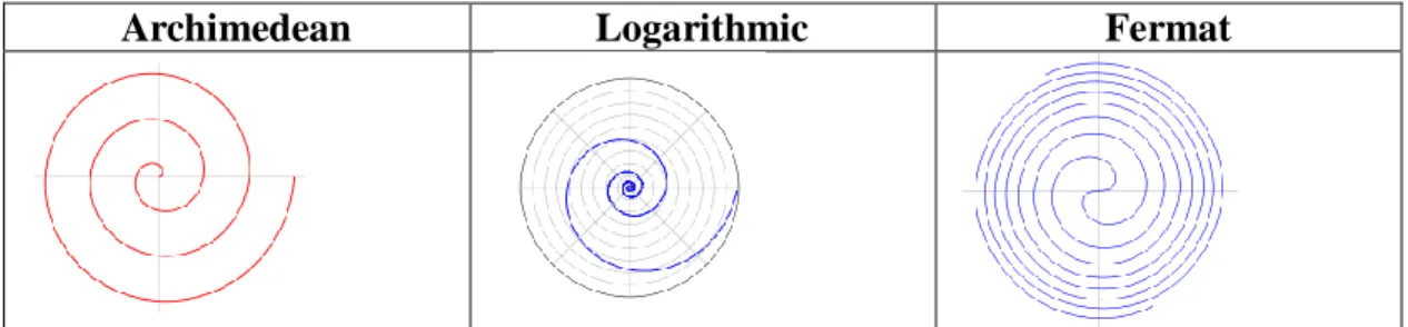
In order to get the binary value of image, an equation is required for extracting its feature. There are a few methods available such as Archimedean spiral, Logarithmic spiral and Fermat spiral. The logarithmic spiral can be distinguished from the spiral by the fact that the distances between the turnings of a logarithmic spiral increase in geometric progression, while in an Archimedean spiral these distances are constant [5].In Archimedean, the path will be rotate away from fixed point with constant angular velocity. Equivalently, in polar coordinates(r, θ) it can be described by the equation

𝑟 = 𝛼 + 𝑏𝜃 (2.1)

with real a and b. Changing the parameter a will turn the spiral, while b controls the distance between successive turnings. Conversely, for Logarithmic spiral, distances between the turnings keep increasing since its angular velocity keep changing. In parametric form, the curve can be defined as

𝑥 x t = rcos t = ae

bt _{cos t}

y t = r sin t = aebt sin t (2.2)

Other equation that can be used is Fermat spiral whereby two spirals with different direction is applied at the same time. The equations are

𝑟2 = 𝑎2𝜃 (2.3)

Figure 1: Spiral Equation to Interpret Image

(15)

2.3K-Nearest Neighbors(KNN) Method

In application, usually we have a description of a texture sample and we want to find which element of database matches that sample. Hence, classification will be needed to associate the appropriate class label (type of texture) with the test sample by using the measurements that describe it. One way to make the association is by finding the member of the class with measurement which differs by the latest amount from the test sample‟s measurement. [8]

For this project, the author will only focus on using K-Nearest Neighbors (KNN) as a method to do pattern recognition. Nearest neighbor is a supervised learning algorithm where the results are classified based on majority of K-nearest neighbor category. The purpose of this algorithm is to classify a new object based on attributes and training samples. KNN technique only requires:

 An integer k

 A set of labeled examples (training data)  A metric to measure “closeness”

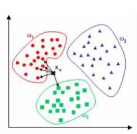
For example, in the figure 2, there are three types of features available which are

𝜔₁,𝜔₂,𝜔₃.We need to identify the class for object 𝑋_𝑢.The classification is using majority vote among the classification of the K objects.[1]Usually Euclidean distance is used as the distance metric yet this is only applicable to continuous variables[3].

(16)

In this case the number of neighbors obtained are 5.Out of them, four are belong to𝜔₁,Therefore,𝑋_𝑢is belong to 𝜔₁ cluster.

Figure 2: Classification Using KNN Technique of Three Different Features

The best choice of value k depends upon the data. Normally, larger values of k reduce the effect of noise on the classification. [2] Training sample is considered as nearest neighbors if the distance of this training sample to the query instance is less than or equal to the K-th smallest distance. In other words, the distance of all training samples will be sorted to the query instance and determine the K-th minimum distance.[4]

2.4K-Means Clustering

The traditional approach of KNN has three limitations that lead to less accurate recognition:[9]

a) High calculation complexity-less number of samples make classifier not optimal while huge number of samples consume more time

b) Dependency on training set-depend on training data excessively. It needs recalculation even if slight changes in training samples

c) No weight difference between samples-all training samples are treated equally without no difference between small number of data with huge number of data

(17)

Therefore, wide varieties of methods have been proposed to deal with this problem. One of them is by using K-means clustering approach.K-means clustering algorithm first was introduced by J. MacQueen(1967) and then by J. A. Hartigan and M.A. Wong around 1975 [1].Generally-means clustering is an algorithm to classify or to group objects based on attributes or features into k number of class. The clustering is evaluated by determining the features that have some similarities between each other and represent it by central point.

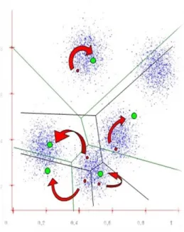
Figure 3: Classification Using improved KNN/Cluster KNN

In the example in figure 3, we divided objects into 5 different group. Each group will consist of random number of data which is relatively close to each other. Each subclass will be represented by one data or more depending on number of subclasses. Then, classification algorithm (nearest neighbors) will be used to classify the representative data. By applying this method, we can reduce the classification time and classification will be more efficient in overlapping area since it takes more consideration to samples of training data that are less frequent.

(18)

CHAPTER 3 METHODOLOGY

3.1Procedure Identification

(19)

3.2Detailed of The Procedure

Throughout this project, there are some procedures that will be followed. This is to ensure that the project can be accomplished within the given timeframe.

3.2.1Data Research and Gathering

The samples that are going to be applied as the input in the algorithm will be gathered from various sources. For the initial stage of this project, the input will be the written alphabets from different people.. The number of training samples of each alphabet will be increased from if necessary to observe the robustness of the algorithm. The author also needs to seek the existing recognition system which related to this project in order to set the bench-mark in term of the accuracy. For the time being, the highest accuracy obtained is 99.21% to 99.95% by using Neural-Network method.[7]

(20)

3.2.2. Image Enhancement

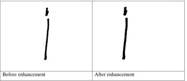
The raw image that been taken from various person may contain certain noise and low quality. Therefore, these images must be enhanced first before being used in the algorithm. One way to improve the quality of image is by using morphological approach. Specific morphological operation will be applied if we use this feature. Its operation can be any of these values:‟bothat‟,‟bridge‟,‟erode‟,‟dilate‟ etc.After implement several test using all the operation‟s value, the author find out that „erode‟ has given he best result on enhancing the image. This operation (erode) will perform dilation using the structuring elements ones (3).

Before enhancement After enhancement

Figure 6: Image Enhancement Using Morphological Operation

From figure 6,it shows that there is some improvement occur on the image whereby the colour depth is getting thicker hence producing clear image. These enhanced images later will be used as the input in algorithm.

(21)

3.2.3Create the Algorithm in Matlab

There are two types of algorithm that are going to be created. The first algorithm will extract feature from training samples and saved in vector form.(Refer Appendix C)

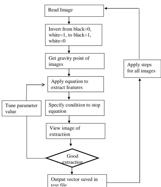
Figure 7: Algorithm to Extract the Features and Convert the Data into Vector Form Apply steps

for all images

Output vector saved in text file

View image of extraction

Specify condition to stop equation

Apply equation to extract features Get gravity point of images

Invert from black=0, white=1, to black=1, white=0 Read Image Tune parameter value Good extraction

(22)

The input images need to be saved in monochrome format and their dimension must be standardized. After that, the image will be read as the input in the matlab by using imread command. Result of this command will give output of the image in 1 and 0 formats. In normal condition zero will represent black while white will represent 1.conversely, normal condition should black to be 1 and white to be zero. Hence,this value will be subtracted with 1 and put in absolute form.. The next step is to find the gravity point of the image. The equation to find gravity point is

𝐺𝑟𝑎𝑣𝑖𝑡𝑦 𝑝𝑜𝑖𝑛𝑡 𝑂_𝐺 = 𝑋𝑖 ,𝑗𝑖 𝑗

𝑛 .𝑚 (3.1)

This gravity point will be the starting point for feature extraction. One of the methods that can be used for feature extraction is spiral equation. The formula are:

𝑋 = 𝑋_𝑔 + 𝑉₀∆ tcos(𝜔∆𝑡)

𝑌 = 𝑌_𝑔 + 𝑉₀∆ tsin(𝜔∆𝑡) (3.2)

The equation will produce an error if no specific condition made to terminate the operation. The equation will break if the curl exceeds the outermost radius of the image or the innermost radius of the image (negative value) .The intersection between image and equation will produce a stream of vector. This vector will be written in text file. This file we will use later in classification phase. All the images will be gone through the same step. At the end of each step, vector need to be saved with different name.

(23)

The second algorithm is to classify the alphabets into their respective cluster. Generally, the program will compute the distance of each vector/image and sort them into their cluster (Refer Appendix G).

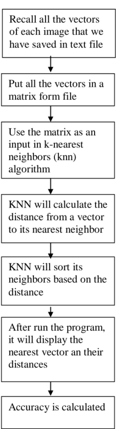
Figure 8: Algorithm to Classify the Image Using KNN Method 01000111000111 01110000110011 00000011111010 01000111000111 01110000110011 00000011111010 Accuracy is calculated KNN will sort its neighbors based on the distance

After run the program, it will display the nearest vector an their distances

Use the matrix as an input in k-nearest neighbors (knn) algorithm

KNN will calculate the distance from a vector to its nearest neighbor Recall all the vectors of each image that we have saved in text file

Put all the vectors in a matrix form file

d1

(24)

In this program, classification will involve the usage of KNN method. First, all the vectors from previous algorithm will be recalled and assign a unique name for each of it.. After that, all the vectors will be arrange together to produce one matrix .This matrix later will be as an input in KNN algorithm. In KNN algorithm, the Euclidean distance of a vector to another will be calculated. Then, the neighbor for each vector will be sorted based on its nearest distance. The user will specify the value of K which is the values of neighbor that they expect to get. After the program is run, it will display the neighbors and distance for each vector. From that, we can calculate the accuracy by determining whether the neighbors are within the expected range or not.

In order to improve the accuracy, parameter values will be tuned, thus the images can be extracted better. Various equations will also being attempted to analyze the best feature extraction method. The equations are linear equation, spiral equation and galaxy equation

3.2.4Cluster K-Nearest neighbors(C-KNN)

Generally, his method aims to classify or group objects based on attributes or features into k number of group. The grouping is done by minimizing the sum of squares of distances between data and corresponding cluster centroid. In order to reduce the time taken for classification, training data must be clustered into subclasses whereby each subclass will be represented by one data. Each subclass contains a random number of data which relatively close to each other. Then, the representative data will be classified using nearest neighbors approach.

(25)

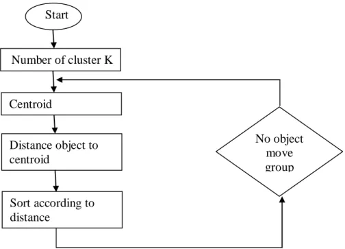
Figure 9: K-means clustering algorithm

The flow of how k-means clustering is being applied is as follow: 1. Determine the value of k(cluster number)

2. Put initial partition that classifies the data into k clusters. The training samples may be assigned randomly or systematically by taking the first k training sample as single element clusters while the remaining samples assigned to cluster with nearest neighbors. After each assignment, the centroid will be recalculated.

3. Take each sample in sequence and compute its distance from the centroid of each cluster. If the samples is not within the cluster of closest centroid,the samples will switch to right cluster. The centroid will be computed once again.

4. Step 3 will be repeated for a few times until convergence is achieved Start Number of cluster K Centroid Distance object to centroid Sort according to distance No object move group

(26)

3.2.5Apply Different Set Of Inputs To Algorithm

In order to increase robustness of classifier, training samples will be added. Besides, a different set of input will also be attempted. By doing this, compatibility of the algorithm with various inputs will be known. The inputs can be signature, object image, human voice and others.

3.2.6Hardware/Application Fabrication And Testing

In the final phase of this project, author supposes to come out with hardware or application that related to real life application. It can be biometric devices to detect fingerprint, iris or palm. The aim to come out with a patentable hardware is to introduce low cost system without neglecting its accuracy.

3.3Tools

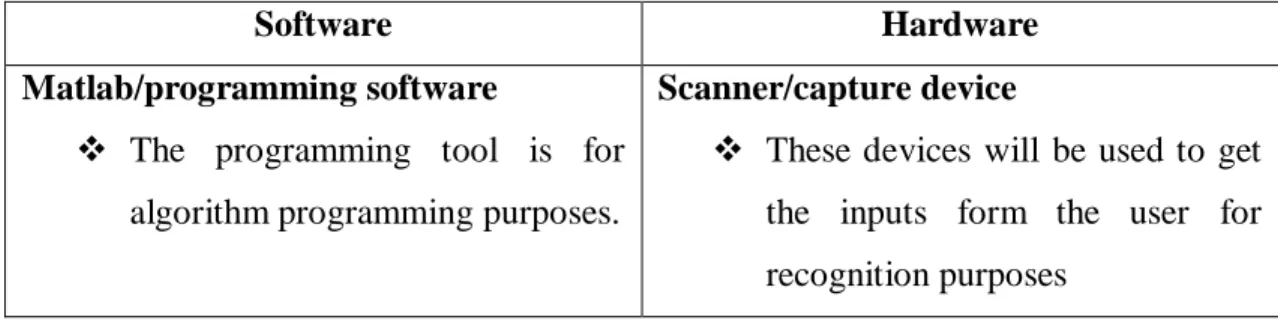
Table 1: List of Hardware and Software Used In This Project

Software Hardware

Matlab/programming software

 The programming tool is for algorithm programming purposes.

Scanner/capture device

 These devices will be used to get the inputs form the user for recognition purposes

(27)

CHAPTER 4 RESULTS AND DISCUSSION

4.1Simulation of algorithm

From the initial phase, the highest accuracy achieved is 82.29% by using dual spiral extraction .The total samples used are written alphabets of a,b,c and d. The number of k is assigned as 3 means sample is accurate if its majority (2/3) of its neighbors are within the desired range. For the next stage, the author has increased the alphabets from a until i. Each alphabet consist of 15 training samples which resulting to total number of sample to 135 images. By adding the training samples, the robustness of algorithm against data size can be analyzed. The feature space of all images will be extracted using various approaches to find out the best solution to produce vector data.

4.1.1Logarithmic Spiral equation

The equation involves in this method are:

𝑋 = 𝑋_𝑔 + 𝑉₀𝛥𝑡𝑐𝑜𝑠 𝜔𝛥𝑡 .

𝑌 = 𝑌_𝑔+ 𝑉₀𝛥𝑡𝑠𝑖𝑛 𝜔𝛥𝑡 . 𝑉0 ≤ 𝜔 (4.1)

Xg and Yg are the starting point of the equation or the gravity point of the images. The manipulated variables involve here are V₀,ω and Δ.An efficient variables should use

(28)

Figure 10: Feature Extraction Using Logarithmic Spiral before Parameter Tuning

From figure 10, we can see that the curl of spiral not good enough since the expansion of curl is too big. Hence, it might cause miss extraction which later will reduce the accuracy of recognition. Therefore, the next step is to tune the parameter in order to improve the formation of spiral

Figure 11: Feature Extraction Using Logarithmic Spiral after Parameter Tuning The consideration made while tune the parameter is ɷ must bigger than 𝑉0.In this

case, the bigger value of ɷ will increase the angular velocity thus increase number of curls. Meanwhile smaller number of 𝑉₀will reduce the speed so compress the distance between each curls.

Gravity point

(29)

4.1.2Fermat Spiral equation

Instead of using single equation, the author attempts to use two equations with different direction. The equation is called Fermat spiral. The second equations implemented are:

𝑋 = 𝑋_𝑔 + 𝑉₀𝛥𝑡𝑐𝑜𝑠 𝜔𝛥𝑡 𝑌 = 𝑌_𝑔 + 𝑉₀𝛥𝑡𝑠𝑖𝑛 𝜔𝛥𝑡 𝑋 = 𝑋_𝑔 + 𝑉₀𝛥𝑡𝑐𝑜𝑠 𝜔𝛥𝑡

𝑌 = 𝑌_𝑔 − 𝑉₀𝛥𝑡𝑠𝑖𝑛 𝜔𝛥𝑡 𝑉0 ≤ 𝜔 (4.2)

Then vector of each equation will be compiled together in an array (Vect_f=[vect_𝑓₁

vect_𝑓2]).The parameter values used are still the same. The accuracy obtained is

slightly less than single spiral.

Logarithmic Spiral Fermat Spiral

Figure 12: Comparison between Feature extraction using Fermat or logarithmic spiral From figure 12,it is proven that the implementation of spiral in both direction will avoid miss-tracing of character. To make the intersection between image and spiral, parameter values must be tuned.

(30)

4.1.3Galaxy Equation

In galaxy, it still uses the spiral equations which are:

𝑋 = 𝑋_𝑔+ 𝑉₀𝛥𝑡𝑐𝑜𝑠 𝜔𝛥𝑡 + 𝜃 .

𝑌 = 𝑌_𝑔+ 𝑉₀𝛥𝑡𝑠𝑖𝑛 𝜔𝛥𝑡 + 𝜃 . 𝑉0 ≫ 𝜔 (4.3)

Xg and Yg are the starting point of the equation or the gravity point of the images. The manipulated variables involve here are V₀,ω and Δ.If we give the value of V₀>>ω,the equation will produce a curve. To make it become a galaxy, curve need to be shifted by certain angle. Let say if we want to have ten curves in the galaxy, the angle shift need to be made by increment of π//5 until it reach 9π /5.

The vector produce by interpretation of each curves will be combined in a vector(Vect_f=[vect_𝑓1….vect_𝑓10])(Refer Appendix E).In order to find the best

formation of galaxy that should be mapped to images, several simulation must be done to find out right number of curl for the galaxy.

Figure 13: Initial Curl For Galaxy Figure 14: Angled –Shifted Curl For Galaxy

(31)

Number of curls:5 Parameter:𝑉₀=500;∆= 0.01; 𝜔 = 1 Accuracy:20.63% Number of curls:9 Parameter:𝑉₀=500;∆= 0.01; 𝜔 = 1 Accuracy:28.57% Number of curls:15 Parameter:𝑉₀=500;∆= 0.01; 𝜔 = 1 Accuracy:25.40%

Figure 15:Feature Extraction Of Images Using Galaxy Equation

Based on the result in figure 15, we can see that the accuracy will reduce if the number of curls is too many. Hence, it is preferable that the number of curls is less so that the error during classification can be reduced.

(32)

4.1.4Dual Galaxy Equation

Instead of using unidirectional galaxy, it is better to use bidirectional galaxy means applied galaxy in forward and backward direction. It is because in one directional galaxy, there is high possibility that the some character miss interpreted by the curl. The equation of dual galaxy is as follow:

𝑋 = 𝑋𝑔+ 𝑉0𝛥𝑡𝑐𝑜𝑠 𝜔𝛥𝑡 + 𝜃 𝑌 = 𝑌_𝑔 + 𝑉₀𝛥𝑡𝑠𝑖𝑛 𝜔𝛥𝑡 + 𝜃 𝑋 = 𝑋_𝑔+ 𝑉₀𝛥𝑡𝑐𝑜𝑠 𝜔𝛥𝑡 + 𝜃

𝑌 = 𝑌_𝑔 − 𝑉₀𝛥𝑡𝑠𝑖𝑛 𝜔𝛥𝑡 + 𝜃 𝑉0 ≫ 𝜔 (4.4)

Unidirectional galaxy Bidirectional galaxy

Figure 16: Comparison Between Unidirectional Galaxy With Bidirectional Galaxy

4.2Accuracy of Recognition

In the initial stage, only 60 samples used consist of 15 each alphabets (a,b,c,d).The highest accuracy achieved previously was 89.29%.For the second phase ,the training samples is added until 135 images. All the methods will be attempted in order to find the most efficient technique to extract the features. Initially, the value of k defined as 3.Thus, if 2 out of 3 neighbors within the expected neighbor‟s range, recognition is considered successful.

(33)

4.3Analysis On Accuracy

From 15 samples of each class, 8 of the images were used for training and other 7 will be used as testing data. In classification phase, two type of classifier will be used which are Euclidean KNN and cluster KNN .For each attempt, parameter value will be tuned to improve the accuracy. Below is the result of analysis done for each method:

Table 2: Result of Accuracy after Parameter Tuning For Logarithmic Spiral

method parameter Accuracy (%) Length

V0 del ω KNN C-KNN Logarithmic spiral 1 0.4 4 77.78 86.7 580 0.1 0.4 5 76.19 91.1 5469 2 0.4 4 79.37 93.3 307 0.1 0.4 7 77.78 91.1 5455 0.1 0.4 10 73.02 95.6 5487 9 0.02 3.5 73.1 93.3 1253 9 0.02 2.5 74.6 93.3 1253 9 0.05 2.5 74.6 91.1 501 9 0.01 2.5 73.02 88.9 2505 9 0.03 2.5 76.2 91.1 835 9 0.02 2.1 61.9 88.9 1266 9 0.02 2.7 65.08 88.9 1274 7 0.02 2.6 76.2 93 1573 7 0.02 2.5 80.9 91 1627 9.5 0.02 2.5 69.8 88.9 1190 9.5 0.02 3.5 76.2 93.3 1167 9.5 0.03 3.9 76 91.1 778 9.5 0.03 4.5 73 93.3 790 9 0.001 2.5 53.97 99 25043 Highest Accuracy 80.9 99

(34)

Table 3: Result of Accuracy after Parameter Tuning For Multiple Spiral

V0 del ω KNN C-KNN Multiple spiral 0.1 0.4 5 69.84 88.9 10947 2 0.4 4 76.19 88.9 614 0.1 0.4 7 69.84 88.9 10917 0.1 0.4 10 73.02 95.6 10983 9 0.02 3.5 66.67 91.1 2505 9 0.02 2.5 69.84 91.1 2505 9 0.05 2.5 66.7 88.9 1001 9 0.01 2.5 69.8 91.1 5009 9 0.03 2.5 69.8 91.1 1669 9 0.02 2.1 65.05 91.1 2531 9 0.02 2.7 61.9 93.3 2547 7 0.02 2.6 68.25 93.3 3197 7 0.02 2.5 68.25 91.1 3253 9.5 0.02 2.5 66.7 88.9 2379 9.5 0.02 3.5 65.1 91.1 2333 9.5 0.03 3.9 66.7 93.3 1555 9.5 0.03 4.5 65.1 93.3 1579 Highest Accuracy 76.19 95.6

For single and double spiral approach, it shown that it cluster KNN method has significantly improve accuracy of recognition. Generally the accuracy for each execution is above 80% with minimal elapsed time. It also concluded that there will be better if the value of ∆ is smaller which mean sampling occur more rapidly during feature extraction.

(35)

Table 4: Result Of Accuracy After Parameter Tuning For Unidirectional Galaxy

V0 del ω KNN C-KNN Galaxy (33 curls) 200 0.05 2 30.16 60 1096 80 0.05 0.2 25.4 56 2740 80 0.5 0.2 14.29 58 292 Galaxy (20 curls) 200 0.05 2 22.2 64 674 80 0.05 0.2 23.8 62 1689 80 0.5 0.2 9.5 44 182 Galaxy (10 curls) 200 0.05 2 42.9 75.6 352 80 0.05 0.2 36.5 60 894 80 0.5 0.2 15.9 49 97 Galaxy (5 curls) 200 0.05 2 38.1 69 193 80 0.05 0.2 34.9 64 508 80 0.5 0.2 15.8 42 57 200 0.01 0.2 28.6 62 958 200 0.5 1 30.2 62 26 Highest Accuracy 42.9 75.6

From table 4,it shows that the lesser number of curls, the higher the accuracy. Furthermore, as the value of Δ become smaller, accuracy also increase. However, in general galaxy approach still not give a satisfactory result in term of accuracy compare to spiral method.

Hence, in order to improve the accuracy, simulation using bidirectional galaxy has been attempted.

(36)

Table 5: Result Of Accuracy After Parameter Tuning For Bidirectional Galaxy

V0 del ω KNN C-KNN Galaxy (33 curls) 200 0.05 2 25.39 53.3 2203 80 0.05 0.2 22.2 46.7 5549 80 0.5 0.2 7.93 42.2 591 Galaxy (20 curls) 200 0.05 2 25.39 51.1 1358 80 0.05 0.2 30.16 51.1 3429 80 0.5 0.2 26.48 33.3 368 Galaxy (10 curls) 200 0.05 2 34.92 60 713 80 0.05 0.2 31.75 53.3 1835 80 0.5 0.2 22.22 35.6 196 Galaxy (5 curls) 200 0.05 2 41.27 55.6 391 80 0.05 0.2 36.5 53.3 1062 80 0.5 0.2 30.16 44.4 114 200 0.01 0.2 47.62 57.8 1877 200 0.5 1 33.3 46.7 51 Highest Accuracy 47.62 60

From table 5, we can conclude that the accuracy slightly increase by using bidirectional approach. It means that some characters that not traced in unidirectional can be overcome if galaxy applied in both directions. However, classification using clusters analysis still unable to give high accuracy as high as spiral method in each trial.

(37)

After attempt all the methods, the author has came out wit the best solution for feature extraction. It can be proved by performing an analysis on average accuracy generated by every method.

Table 6: Average Accuracy Produced By Each Method for KNN and C-KNN

methods Average accuracy KNN C-KNN Logarithmic spiral 73.09 91.73 Fermat Spiral 68.12 91.23 Unidirectional galaxy 26.3 59.11 Bidirectional galaxy 29.66 48.9

Figure 17: Graph of Average Accuracy For Each Methods

From the graph, it is concluded that only Logarithmic spiral and Fermat spiral reach the average accuracy of 90% by using C-KNN classifier. Hence, either Logarithmic or Fermat spiral is the most optimal approach for feature extraction.

(38)

Table 7: Effect On Accuracy While Varying K Values K Accuracy Single spiral Multiple spiral unidirectional galaxy Bidirectional galaxy 1 82 84 52 54 3 73 73 43 47.6 5 73 64 38 38.1 7 60 57 32 30.2 9 54 52 25 23.8

Figure 18: Analysis on Accuracy When Varying K Value

For each approach, the optimal parameter values used while varying the value of k .According to figure 17,it shows that the accuracy is inversely proportional with k values. As we increase the k values, the accuracy decrease. Thus, it is recommended that the value of k assigned is small to get the optimal result.

0 10 20 30 40 50 60 70 80 90 1 3 5 7 9 A cc u ra cy

Accuracy vs. k values

single spiral multiple spiral unidirectional galaxy bidirectional galaxy

(39)

4.4Graphical User Interface(GUI) Application

A user-friendly Graphic User Interface (GUI) is built to integrate the classification module with database of written alphabets. By having this application, it will assist the user to apply character recognition system to their real application. Through the GUI the user can insert an image of alphabet. This new image can be classified to its respective cluster by referring to the database. The user may choose to use any approach such as single spiral, multiple spiral, unidirectional galaxy or bidirectional galaxy for feature extraction. Lastly, the class those image belong to will appear.

(40)

4.5Problem Encountered & Future Planning

The accuracy achieved so far is still low compare to author‟s target which is 99.21% to 99.95% by using Neural-Network method.[7].Besides, result also inconsistent for every execution and still searching for the solemnly factor that affect accuracy. For instance, if the period of sampling Δ is too small it will cause low accuracy recognition. Thus, spiral with very short sampling not necessarily gives the good result. In addition, the size of vector still big and will consume more time for classification.

For the future work, it is recommended to attempt another input data to the algorithm. From that, we can analyze the degree of robustness for the classifier. For instance, the algorithm can be applied for signature recognition to record the attendance. The user will insert their signature into system. After that, the system will register the user into attendance record. The application will also preview the details of the user.The overview of the application can be seen below:

(41)

CHAPTER 5 CONCLUSION AND RECOMMENDATIONS

5.1Conclusion

Artificial Intelligent plays an important role in today‟s life. There are various approaches on pattern recognition. However-Nearest Neighbors (KNN) method is more preferable since it is simple and has faster execution time. The crucial aspect in pattern recognition is its accuracy since this system is widely used for safety purposes. The other idea of this project is to reduce the data size by shorten vector form representation of the image using simple feature extraction approach. If the vector size is too big, it will take longer time to being classified. Moreover, it also tends to produce error in classification by misplace the right class that objects belong to. After implementing all four extraction methods, the most efficient result is using single/logarithmic spiral. The Highest accuracy achieved throughout this project is 99.05 %.The user interface window has been developed in order to ease the user to utilize the algorithm.

(42)

5.2Recommendations

Since the accuracy produced by certain approach is still unsatisfactory, thus the author need to keep on doing the improvisation on the algorithm in order to increase the plausibility of the recognition. The easiest way to improve the recognition is by tuning the parameter value (V₀, ω, Δ) for feature extraction. Assignation of the value can vary depending on the method used to get the features. Other than that, there are few suggested methods or additional algorithm that can be implemented to increase the accuracy.

5.2.1 Variance-modified Methods

This method used to enhance the accuracy of recognition. We can use Gaussian approximation variables for each execution of algorithm to obtained the highest accuracy

𝑃 𝑒𝑟𝑟𝑜𝑟 𝑥 = 𝑃 𝑥 ∈ 𝑐𝑙𝑎𝑠𝑠𝑖 , 𝑃( 𝑒𝑟𝑟𝑜𝑟 𝑥 ∈ 𝑐𝑙𝑎𝑠𝑠𝑖) 2 𝑖=1 (5.1)

5.2.2Genetic K-Nearest Neighbors Method

Genetic algorithm (GA) is combined with K-nearest neighbors algorithm called G-KNN to overcome the limitation of traditional KNN. By using GA, k-number of samples are chosen for each iteration and the classification accuracy is calculated as fitness. The highest accuracy is recorded each time thus avoid the calculation of similarities between each sample.[9]

(43)

REFERENCES

[1] KardiTeknomo,K-Nearest Neighbor Tutorial [journal]-Japan, Graduate School of Information Sciences, 2006

[2] Yang Song,JianHuangDingZhou,HongyuanZha,Lee Giles

IKNN:Informative K-Nearest Neighbor Pattern Classification[Journal]-university Park,PAUSA.

[3] David Bremner, Erik Demaine, Jeff Erickson, John Iacono, Stefan Langerman, Pat Morin, and Godfried Toussaint, Output-sensitive algorithms for computing nearest-neighbor decision boundaries, Discrete and Computational Geometry[book]-New Jersey,John Wiley and Sons Inc,2005,Vol. 33

[4] Richard O. Duda, Peter E. Hart, David G. Stork Pattern classification [book]-New York,Wiley,2001,2nd edition

[5] Beyer, W. H.CRC Standard Mathematical Tables,.Boca Raton, FL: CRC Press, p. 225, 1987, 28th edition

[6] Li Baoli, Yu Shiwen, and Lu Qin,”An Improved k-Nearest Neighbor Algorithm for Text Categorization”[journal]-Institute of Computational Linguistics Department of Computer Science and Technology PekingUniversity, Beijing, P.R. China

(44)

[7] Steffen Wachenfeld, Sebastian Terlunen, XiaoyiJiang,”Robust Recognition of 1-D Barcodes Using Camera Phones”[journal] Computer Vision and Pattern Recognition Group, Department of Computer Science, University of Munster, Germany

[8] Mark Nixon,AlbertoAguado,Feature Extraction & Image Processing[book]-Oxford,Newness,p.301 2002,1st Edition

[9] N. Suguna,Dr K. Thanushkodi,”Improved k-Nearest neighbors Classification Using Genetic Algorithm”[journal]-Computer Science and Engineering,Akshaya College of Engineering and Technology,Coimbatore,TamilNadu,India

[10] Avi Drissman,Dr. Sethi, “Handwriting Recognition Systems: An Overview”[journal]-CSC 496,India

[11] Shashank Araokar, Visual Character Recognition Using Artificial Neural Network” [journal]-Electronics and telecommunication,University of Mumbai,India

[12] L.Harmon.”automatic recognition of print and script.Proc.”IEE,60:1165–1176, 1972.

[13] Dongxiao N., Zhihong G., Xing M. 2007, “Research on Neural Networks Based on Culture Particle Swarm Optimization and Its Application in Power Load Forecasting” Natural Computation, ICNC 2007. Third International Conference, vol.1, pp. 2700274.

[14] D. M. Titterington, A. F. M. Smith, and U. E. Makov, Statistical Analysis of Finite Mixture Distributions.John Wiley, New York, 1985

(45)

[15] X. Jia and J. A. richards, “Fast k-NN classification Using the Cluster-Space Approach”, IEEE Trans., Geosci. Remote Sens., vol. 2, no. 2, April 2005.

(46)

(47)

APPENDIX A

GANTT CHART FOR FYP 1

APPENDIX B

(48)

APPENDIX C

SOURCE CODE IN MATLAB FOR LOGARITHMIC SPIRAL EQUATION

clearall;

x=imread('A1.bmp');%A1-A7,B1-B8,C1-C5,D1-D8,E1-E5

x=abs(x-1); [n_xm_x]=size(x);

%%%% next step is finding the gravity point adx=0; for i=1:n_x for j=1:m_x adx=adx+i*x(i,j); end end g_x=adx/sum(sum(x~=0)); adx=0; for i=1:n_x for j=1:m_x adx=adx+j*x(i,j); end end g_y=adx/sum(sum(x~=0)); gravity=[n_xm_x; g_xg_y] V0=1; del=0.4;w=4;

N=round( max(g_x/(V0*del),g_y/(V0*del)) + min((n_x-g_x)/(V0*del),(m_x-g_y)/(V0*del)) )/2; vect_f(1)=x(round(g_x+(V0*del*0*cos(w*del*0))),round(g_y+(V0*del*0*sin(w*del*0)))) ; for T=1:N if round(g_x+(V0*del*T*cos(w*del*T)))<=0 break; end if round(g_y+(V0*del*T*sin(w*del*T)))<=0 break; end if round(g_x+(V0*del*T*cos(w*del*T)))>n_x break; end if round(g_y+(V0*del*T*sin(w*del*T)))>m_x break; end vect_f=[vect_f x(round(g_x+(V0*del*T*cos(w*del*T))),round(g_y+(V0*del*T*sin(w*del*T))))]; end [mx posit]=sort(vect_f); siz_L=size(vect_f, 2); vect_f(posit(siz_L)+1:siz_L)=[];

fid = fopen('vect_A1.txt','wt');

fwrite(fid,vect_f,'float');

fclose(fid); size(vect_f)

(49)

APPENDIX D

ADDITIONAL CODE FOR FERMAT SPIRAL EQUATION

V0=1; del=0.4;w=4;

N=round( max(g_x/(V0*del),g_y/(V0*del)) + min((n_x-g_x)/(V0*del),(m_x-g_y)/(V0*del)) )/2;

%%%%% apply spiral equation in reverse rotation

vect_fr(1)=x(round(g_x+(V0*del*0*cos(w*del*0))),round(g_y-(V0*del*0*sin(w*del*0)))); for T=1:N if round(g_x+(V0*del*T*cos(w*del*T)))<=0 break; end if round(g_y-(V0*del*T*sin(w*del*T)))<=0 break; end if round(g_x+(V0*del*T*cos(w*del*T)))>n_x break; end if round(g_y-(V0*del*T*sin(w*del*T)))>m_x break; end vect_fr=[vect_fr x(round(g_x+(V0*del*T*cos(w*del*T))),round(g_y-(V0*del*T*sin(w*del*T))))]; end

%%%%% apply spiral equation in forward rotation

vect_ff(1)=x(round(g_x+(V0*del*0*cos(w*del*0))),round(g_y+(V0*del*0*sin(w*del*0)))); for T=1:N if round(g_x+(V0*del*T*cos(w*del*T)))<=0 break; end if round(g_y+(V0*del*T*sin(w*del*T)))<=0 break; end if round(g_x+(V0*del*T*cos(w*del*T)))>n_x break; end if round(g_y+(V0*del*T*sin(w*del*T)))>m_x break; end vect_ff=[vect_ff x(round(g_x+(V0*del*T*cos(w*del*T))),round(g_y+(V0*del*T*sin(w*del*T))))]; end

%%%%% arrange the vector in an array vect_f=[vect_ffvect_fr];

vect_f=[vect_ffvect_fr]; [mx posit]=sort(vect_f); siz_L=size(vect_f, 2);

vect_f(posit(siz_L)+1:siz_L)=[];

fid = fopen('vect_A1.txt','wt');

fwrite(fid,vect_f,'float');

(50)

APPENDIX E

ADDITIONAL CODE FOR UNIDIRECTIONAL GALAXY

c=bwmorph(x,'erode'); c=abs(c-1);

[n_x m_x]=size(c);

%%%% next step is findind the gravity point

adx=0; for i=1:n_x for j=1:m_x adx=adx+i*c(i,j); end end g_x=adx/sum(sum(c~=0)); adx=0; for i=1:n_x for j=1:m_x adx=adx+j*c(i,j); end end g_y=adx/sum(sum(c~=0)); gravity=[n_x m_x; g_x g_y] parameter(); Graph_function=zeros(size(c)); final_pt=round( max((n_x-g_x)/(V0*del),(m_x-g_y)/(V0*del)) ); vect_ff=0; for j_a=0:n_g for T=0:1:final_pt if (round(g_x+(V0*del*T*cos((w*del*T+(2*pi*j_a)/n_g))))>0)&(round(g_y+(V0*del*T*sin((w*del*T+(2*pi*j_a)/n_g))))>0)&(r ound(g_x+(V0*del*T*cos((w*del*T+(2*pi*j_a)/n_g))))<=n_x)&(round(g_y+(V0*del*T*sin((w*del*T+(2*pi*j_a)/n_g))))<=m _x) Graph_function(round(g_x+(V0*del*T*cos(w*del*T+(2*pi*j_a)/n_g))),round(g_y+(V0*del*T*sin(w*del*T+(2*pi*j_a)/n_g))) )=1; vect_ff=[vect_ff c(round(g_x+(V0*del*T*cos(w*del*T+(2*pi*j_a)/n_g))),round(g_y+(V0*del*T*sin(w*del*T+(2*pi*j_a)/n_g))))]; end end end vect_f=[vect_ff]; [mx posit]=sort(vect_f); siz_L=size(vect_f, 2); vect_f(posit(siz_L)+1:siz_L)=[];

(51)

APPENDIX F

ADDITIONAL CODE FOR BIDIRECTIONAL GALAXY

c=bwmorph(x,'erode'); c=abs(c-1); [n_x m_x]=size(c); adx=0; for i=1:n_x for j=1:m_x adx=adx+i*c(i,j); end end g_x=adx/sum(sum(c~=0)); adx=0; for i=1:n_x for j=1:m_x adx=adx+j*c(i,j); end end g_y=adx/sum(sum(c~=0)); gravity=[n_x m_x; g_x g_y] parameter(); Graph_function=zeros(size(c)); final_pt=round( max((n_x-g_x)/(V0*del),(m_x-g_y)/(V0*del)) ); vect_ff=0; for j_a=0:n_g for T=0:1:final_pt if (round(g_x+(V0*del*T*cos((w*del*T+(2*pi*j_a)/n_g))))>0)&(round(g_y+(V0*del*T*sin((w*del*T+(2*pi*j_a)/n_g))))>0)&(r ound(g_x+(V0*del*T*cos((w*del*T+(2*pi*j_a)/n_g))))<=n_x)&(round(g_y+(V0*del*T*sin((w*del*T+(2*pi*j_a)/n_g))))<=m _x) Graph_function(round(g_x+(V0*del*T*cos(w*del*T+(2*pi*j_a)/n_g))),round(g_y+(V0*del*T*sin(w*del*T+(2*pi*j_a)/n_g))) )=1; vect_ff=[vect_ff c(round(g_x+(V0*del*T*cos(w*del*T+(2*pi*j_a)/n_g))),round(g_y+(V0*del*T*sin(w*del*T+(2*pi*j_a)/n_g))))]; end end end for j_a=0:n_g for T=0:1:final_pt if (round(g_x+(V0*del*T*cos((w*del*T+(2*pi*j_a)/n_g))))>0)&(round(g_y-(V0*del*T*sin((w*del*T+(2*pi*j_a)/n_g))))>0)&(round(g_x+(V0*del*T*cos((w*del*T+(2*pi*j_a)/n_g))))<=n_x)&(round(g_ y-(V0*del*T*sin((w*del*T+(2*pi*j_a)/n_g))))<=m_x) Graph_function(round(g_x+(V0*del*T*cos(w*del*T+(2*pi*j_a)/n_g))),round(g_y-(V0*del*T*sin(w*del*T+(2*pi*j_a)/n_g))))=1; vect_ff=[vect_ff x(round(g_x+(V0*del*T*cos(w*del*T+(2*pi*j_a)/n_g))),round(g_y-(V0*del*T*sin(w*del*T+(2*pi*j_a)/n_g))))]; end end end

(52)

APPENDIX G

SOURCE CODE IN MATLAB FOR CLASSIFICATION

clear all;

fid = fopen('vect_A1.txt','rt') vect_A1=fread(fid,'float') fclose(fid)

fid = fopen('vect_B1.txt','rt') vect_B1=fread(fid,'float') fclose(fid)

(53)

vect_B4=fread(fid,'float') fclose(fid)

fid = fopen('vect_C1.txt','rt') vect_C1=fread(fid,'float') fclose(fid)

(54)

fclose(fid)

fid = fopen('vect_D1.txt','rt') vect_D1=fread(fid,'float') fclose(fid)

fid = fopen('vect_E1.txt','rt') vect_E1=fread(fid,'float') fclose(fid)

(55)

fid = fopen('vect_F1.txt','rt') vect_F1=fread(fid,'float') fclose(fid)

fid = fopen('vect_F9.txt','rt') vect_F9=fread(fid,'float')

(56)

vect_F10=fread(fid,'float') fclose(fid)

fid = fopen('vect_G1.txt','rt') vect_G1=fread(fid,'float') fclose(fid)

fid = fopen('vect_H1.txt','rt') vect_H1=fread(fid,'float') fclose(fid)

fid = fopen('vect_H2.txt','rt') vect_H2=fread(fid,'float')

(57)

fclose(fid)

fid = fopen('vect_I1.txt','rt') vect_I1=fread(fid,'float') fclose(fid)

(58)

fid = fopen('vect_I15.txt','rt'); vect_I15=fread(fid,'float'); fclose(fid)

n=max([size(vect_A1,1),size(vect_A2,1), size(vect_A3,1),size(vect_A4,1), size(vect_A5,1) ,size(vect_A6,1),size(vect_A7,1),size(vect_A8,1), size(vect_A9,1),size(vect_A10,1),

size(vect_A11,1),size(vect_A12,1),size(vect_A13,1),size(vect_A14,1),size(vect_A15,1),size(vect_B1,1),size(vect_B2,1), size(vect_B3,1),size(vect_B4,1), size(vect_B5,1) ,size(vect_B6,1),size(vect_B7,1),size(vect_B8,1),

size(vect_B9,1),size(vect_B10,1),

size(vect_B11,1),size(vect_B12,1),size(vect_B13,1),size(vect_B14,1),size(vect_B15,1),size(vect_C1,1),size(vect_C2,1), size(vect_C3,1),size(vect_C4,1), size(vect_C5,1) ,size(vect_C6,1),size(vect_C7,1),size(vect_C8,1),

size(vect_C9,1),size(vect_C10,1),

size(vect_C11,1),size(vect_C12,1),size(vect_C13,1),size(vect_C14,1),size(vect_C15,1),size(vect_D1,1),size(vect_D2,1), size(vect_D3,1),size(vect_D4,1), size(vect_D5,1) ,size(vect_D6,1),size(vect_D7,1),size(vect_D8,1),

size(vect_D9,1),size(vect_D10,1), size(vect_D11,1),size(vect_D12,1),size(vect_D13,1),size(vect_D14,1),size(vect_D15,1),size(vect_E1,1),size(vect_E2,1),size(ve ct_E3,1),size(vect_E4,1),size(vect_E5,1),size(vect_E6,1),size(vect_E7,1),size(vect_E8,1),size(vect_E9,1),size(vect_E10,1),siz e( vect_E11,1),size(vect_E12,1),size(vect_E13,1),size(vect_E14,1),size(vect_E15,1),size(vect_E15,1),size(vect_E15,1),size(vect_ E15,1),size(vect_E15,1),size(vect_F1,1),size(vect_F2,1),size(vect_F3,1),size(vect_F4,1),size(vect_F5,1),size(vect_F6,1),size( ve ct_F7,1),size(vect_F8,1),size(vect_F9,1),size(vect_F10,1),size(vect_F11,1),size(vect_F12,1),size(vect_F13,1),size(vect_F14,1),s ize(vect_F15,1),size(vect_G1,1),size(vect_G2,1),size(vect_G3,1),size(vect_G4,1),size(vect_G5,1),size(vect_G6,1),size(vect_G7 ,1),size(vect_G8,1),size(vect_G9,1),size(vect_G10,1),size(vect_G11,1),size(vect_G12,1),size(vect_G13,1),size(vect_G14,1),size (vect_G15,1),size(vect_H1,1),size(vect_H2,1),size(vect_H3,1),size(vect_H4,1),size(vect_H5,1),size(vect_H6,1),size(vect_H7,1) ,size(vect_H7,1),size(vect_H8,1),size(vect_H9,1),size(vect_H10,1),size(vect_H11,1),size(vect_H12,1),size(vect_H13,1),size(ve ct_H14,1),size(vect_H15,1),size(vect_I1,1),size(vect_I2,1),size(vect_I3,1),size(vect_I4,1),size(vect_I5,1),size(vect_I6,1),si ze(ve ct_I7,1),size(vect_I8,1),size(vect_I9,1),size(vect_I10,1),size(vect_I11,1),size(vect_I12,1),size(vect_I13,1),size(vect_I14,1),size( vect_I15,1)]); v1=zeros(n,1); v2=zeros(n,1); v3=zeros(n,1); v4=zeros(n,1); v5=zeros(n,1); v6=zeros(n,1); v7=zeros(n,1); v8=zeros(n,1); v9=zeros(n,1); v10=zeros(n,1); v11=zeros(n,1); v12=zeros(n,1); v13=zeros(n,1); v14=zeros(n,1); v15=zeros(n,1); v16=zeros(n,1); v17=zeros(n,1); v18=zeros(n,1); v19=zeros(n,1); v20=zeros(n,1); v21=zeros(n,1); v22=zeros(n,1); v23=zeros(n,1);

(59)

v24=zeros(n,1); v25=zeros(n,1); v26=zeros(n,1); v27=zeros(n,1); v28=zeros(n,1); v29=zeros(n,1); v30=zeros(n,1); v31=zeros(n,1); v32=zeros(n,1); v33=zeros(n,1); v34=zeros(n,1); v35=zeros(n,1); v36=zeros(n,1); v37=zeros(n,1); v38=zeros(n,1); v39=zeros(n,1); v40=zeros(n,1); v41=zeros(n,1); v42=zeros(n,1); v43=zeros(n,1); v44=zeros(n,1); v45=zeros(n,1); v46=zeros(n,1); v47=zeros(n,1); v48=zeros(n,1); v49=zeros(n,1); v50=zeros(n,1); v51=zeros(n,1); v52=zeros(n,1); v53=zeros(n,1); v54=zeros(n,1); v55=zeros(n,1); v56=zeros(n,1); v57=zeros(n,1); v58=zeros(n,1); v59=zeros(n,1); v60=zeros(n,1); v61=zeros(n,1); v62=zeros(n,1); v63=zeros(n,1); v64=zeros(n,1); v65=zeros(n,1); v66=zeros(n,1); v67=zeros(n,1); v68=zeros(n,1); v69=zeros(n,1); v70=zeros(n,1); v71=zeros(n,1); v72=zeros(n,1); v73=zeros(n,1); v74=zeros(n,1); v75=zeros(n,1); v76=zeros(n,1); v77=zeros(n,1); v78=zeros(n,1); v79=zeros(n,1); v80=zeros(n,1); v81=zeros(n,1); v82=zeros(n,1); v83=zeros(n,1); v84=zeros(n,1); v85=zeros(n,1); v86=zeros(n,1); v87=zeros(n,1); v88=zeros(n,1);

(60)

v91=zeros(n,1); v92=zeros(n,1); v93=zeros(n,1); v94=zeros(n,1); v95=zeros(n,1); v96=zeros(n,1); v97=zeros(n,1); v98=zeros(n,1); v99=zeros(n,1); v100=zeros(n,1); v101=zeros(n,1); v102=zeros(n,1); v103=zeros(n,1); v104=zeros(n,1); v105=zeros(n,1); v106=zeros(n,1); v107=zeros(n,1); v108=zeros(n,1); v109=zeros(n,1); v110=zeros(n,1); v111=zeros(n,1); v112=zeros(n,1); v113=zeros(n,1); v114=zeros(n,1); v115=zeros(n,1); v116=zeros(n,1); v117=zeros(n,1); v118=zeros(n,1); v119=zeros(n,1); v120=zeros(n,1); v121=zeros(n,1); v122=zeros(n,1); v123=zeros(n,1); v124=zeros(n,1); v125=zeros(n,1); v126=zeros(n,1); v127=zeros(n,1); v128=zeros(n,1); v129=zeros(n,1); v130=zeros(n,1); v131=zeros(n,1); v132=zeros(n,1); v133=zeros(n,1); v134=zeros(n,1); v135=zeros(n,1); v1(1:size(vect_A1,1))=vect_A1; v2(1:size(vect_A2,1))=vect_A2; v3(1:size(vect_A3,1))=vect_A3; v4(1:size(vect_A4,1))=vect_A4; v5(1:size(vect_A5,1))=vect_A5; v6(1:size(vect_A6,1))=vect_A6; v7(1:size(vect_A7,1))=vect_A7; v8(1:size(vect_A8,1))=vect_A8; v9(1:size(vect_A9,1))=vect_A9; v10(1:size(vect_A10,1))=vect_A10; v11(1:size(vect_A11,1))=vect_A11; v12(1:size(vect_A12,1))=vect_A12; v13(1:size(vect_A13,1))=vect_A13; v14(1:size(vect_A14,1))=vect_A14; v15(1:size(vect_A15,1))=vect_A15; v16(1:size(vect_B1,1))=vect_B1; v17(1:size(vect_B2,1))=vect_B2; v18(1:size(vect_B3,1))=vect_B3; v19(1:size(vect_B4,1))=vect_B4; v20(1:size(vect_B5,1))=vect_B5;