Charging facility allocation in smart cities

(1)

c

(2)

CHARGING FACILITY ALLOCATION IN SMART CITIES

BY

SITING CHANG

THESIS

Submitted in partial fulfillment of the requirements for the degree of Master of Science in Computer Science

in the Graduate College of the

University of Illinois at Urbana-Champaign, 2016

Urbana, Illinois Adviser:

(3)

ABSTRACT

The raising concerns of energy consumption and air pollution advance the development of electric vehicle technologies and promote the increased de-ployment of Electric Vehicles (EVs) towards electric transportation. The increasing number of EVs on the road network leads to a growing challenge of electricity management for the power grid to promptly supply electricity to EVs. In order to address this challenge, we need to carefully plan the energy sources and energy delivery via charging facilities to EVs, taking into consideration interdependencies between roads/transportation and electric grid. In this thesis, we focus on studying the placement of energy sources and their charging facilities for EVs by developing: 1) an extended Flow Re-fueling Location model [1] which finds optimal locations for charging stations as well as dynamic wireless charging pads, and 2) a 2-stage planning process for placement of charging stations [2]. The first stage of the planning process is to determine the optimal locations for placing the charging stations to serve the maximum amount of EVs on the road network. Given the selected optimal locations, the second stage determines the capacity of the charging service locations with the purpose of minimizing the total waiting time of EV drivers across the road network to charge their EVs. We show the effec-tiveness of these two planning models on a sample road network during our performance evaluation.

(4)

CHAPTER 1 INTRODUCTION

Major concerns regarding energy consumption and air pollution lead to the development of electricity powered vehicles. Pure Electric Vehicle (EV) and Plugin Hybrid Electric Vehicle (PHEV) are two main types of vehicles that are promoted to replace conventional fossil consuming vehicles [3]. Their market penetration will experience a significant increase in the following years [4, 5] as studies in various fields related to EV [6, 7, 8, 9] show. Due to the limitation of driving range of a charged EV, the accessibility of public charging facilities is one key issue that restricts the widespread adoption of EVs [10].

As we can see from Figure 1.2, which presents the available public charging stations for EVs in U.S. in year 2013, the accessibility of charging stations is far from evenly distributed across the nation and the accessibility to charging stations is extremely limited in the central area. Therefore, carefully placed and planned charging stations as well as other types of charging facilities are in great needs in the following years in order to support and promote the mass adoption of EVs. Motived by the increasing demand of charging facilities, this thesis focuses on studying the charging facility allocation problem in cities.

Charging station is one of the most widely adopted charging facilities on road network. However, the risks and concerns of charging stations such as electrocution advance the development of an inductive charging technique which is applied by charging pad [13]. Figure 1.2 shows an example of a road segment which is equipped with dynamic wireless charging pads that charges electric bus on the fly. In Chapter 2, we introduce and compare the charging facilities in more detail.

We propose a model, called an extended Flow Refueling Location Model, as an optimization problem to find optimal locations for 2 types of charging facilities: charing stations and dynamic wireless charging pads with the goal

(6)

Figure 1.1: Available charging stations for electric vehicles in U.S. in year 2013 [11].

Figure 1.2: Illustration of wireless dynamic charging pads for electric buses [12].

(7)

of maximizing the number of EVs that could be charged on the road network [1]. Furthermore, we propose a 2-stage planning process for charging sta-tions. The first stage applies the extended Flow Refueling Location Model which was designed to find optimal locations both for charging stations and dynamic wireless charging pads. After obtaining the optimal locations, one critical question remains to answer is the configuration plan for the allocated charging facilities. The specific configuration plans depend on the type of charging facilities allocated. For example, let us assume it is optimal to pick a road link to deploy dynamic wireless charging pads, we then need to de-termine how long should we pave the charging pads. In terms of charging stations, we need to answer questions such as how many charging servers should we deploy for each station. Note that charging servers are the access-handles for EVs to connect to the energy source within (or close to) the charging station. EV needs to obtain a charging server to get charged which is similar to conventional vehicles requiring handles to get served at a gas station.

Each charging station could have more than one charging server and the number of charging servers deployed in each charging station affects the per-formance of the charging facility system since

• it determines the service rate for each charging station which will there-fore affect the waiting time of EV drivers and the charging completion rate (i.e., the ratio between the number of vehicles successfully charged and the total number of arrived EVs) of the charging system,

• it determines the maximum number of EVs that could be charged at the same time which will affect the power grid system since charging a large number of EVs leads to peaks of electricity supplying demand which puts a high pressure on the power grid infrastructure. Therefore, we need to make sure the demand peak will not collapse the whole power grid system.

As stated above, it is essential to study the configuration plan for charging facilities in order to complete the facility planning research. Thus, the goal of the second stage is exploring the optimal configuration plan for charging facilities. However, due to the fact that dynamic wireless charging pads are not yet widely adopted on the road network, its related configuration

(8)

planning has not raised a big concern. Thus, in this thesis, we only focus on discussing the configuration planning for charging stations.

Therefore, the first stage adopts and customizes the extended FRLM model proposed in [1] to find optimal locations for charging stations under a budget constraint and the second stage next explores the optimal configuration plan based on the optimal locations obtained from the first stage.

In this thesis, we present our work on charging facility planning and our contributions are:

• We acknowledge the differences between various types of charging fa-cilities and discuss the concerns and challenges when allocating these types of charging facilities on road networks.

• We propose a model, the extended FRLM [1], to find optimal locations for charging facilities when two different types of facilities are taken into consideration. In particular, we focus on studying placing charging stations and dynamic wireless charging pads.

• We propose a 2-stage planning process for charging station planning [2]. The first stage starts by choosing the optimal locations for charging stations from the macroscopic view and the second stage focuses on the configuration plan of charging servers for each charging station from the microscopic view point.

• We discuss lessons learned when studying the charging facility alloca-tion problem. We also present a list of interesting and open topics worth exploring in the future.

The thesis is structured as follows: detailed introduction and comparison regarding different types of charging facilities are presented in Chapter 2; in Chapter 3, we introduce the background knowledge, concepts and notations we use throughout this thesis, as well as presenting a detailed description of the problem; in Chapter 4, we review related work on the charging facility allocation problem. In Chapter 5, we review the FRLM proposed in [14] and in Chapter 6, we introduce our proposed Extended FRLM. In Chapter 7, we present the 2-stage planning process. Evaluation results are presented in Chapter 8. In Chapter 9, we discuss the lessons learned and challenges encountered when studying the charging facility allocation problem. At last, in Chapter 10, we conclude the thesis and present potential future work.

(9)

CHAPTER 2 CHARGING FACILITIES

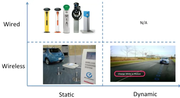
In this chapter, we introduce the background of EV charging with a focus on charging facilities. Depending on the various working principles of charging facilities, the charging facilities can mainly be categorized into 2 categories: wired and wireless charging facilities. In the following sections, we review these two types of facilities separately. At the end of the chapter, we discuss the challenges and concerns when placing charging facilities on road networks.

2.1 Wired charging

Wired charging primarily refers to charging stations which are also the most widely adopted charging facilities for EVs. Gas stations refill conventional vehicles when vehicles arrive in stations and obtain a gas pump. In the same manner, charging stations charge EVs as shown in Figure 2.1 1. More specifically, an EV arrives at a charging station, obtains a charging server (by parking car next to the charging server), and starts charging to a satisfactory level to support its later trip. As mentioned in Chapter 1, charging servers are access points for EVs to the energy source and one charging station can include one or more charging servers (i.e. also multiple parking lots).

Depending on the publicity of charging stations, stations could be classified into personal and public charging stations. A personal charging station refers to a charging station served in xxx installed at the EV owner’s home, where EV owner charges the vehicle overnight. On the other hand, public charging stations are built in public parking spaces which are accessible to all EVs.

According to the charging rate of charging stations, stations could be cat-egorized into AC level 1 charging and fast charging (such as AC level 2 and

1_{Note that gas stations are isolated physical infrastructures to enable XXXX of gasoline}

in safe manner. Charging station is becoming an XXXX part of a parking facility close to a major point of interest, such as mall, downtown entertainment area and others.

(10)

Figure 2.1: Illustration of charging station of electric vehicles [15]. level 3) [16]. EVs takes advantage of AC level 1 charging by connecting to a standard home or business outlet through a 120-volt alternating-current plug. AC level 2 provides charging through 208/240-volt alternating-current charging equipment while AC level 3, also referred to as DC fast charging, provides charging at 480VAC. Typically, there is no installation of charging equipment required for AC level 1 charging and depending on the model of an EV, it could take 8 to 20 hours to fully charge the vehicle. However, for fast charging options, specific charging equipment is required. For AC level 2 charging, depending on the model of an EV, it could take 4 to 8 hours to charge an EV and it takes approximately 10 to 30 minutes to recharge an EV using the AC level 3 charging.

2.2 Wireless charging

Wireless charging facilities charge EVs wirelessly and wireless charging can be further categorized into static wireless charging and dynamic wireless charging.

EVs can get charged by parking over a static wireless charging pad as described in Figure 2.2a. Static wireless charging requires installment of: 1) a wireless charging pad on the ground, 2) a control panel, and 3) an adapter

(11)

(a) Illustration of static wireless charging [20].

(b) Illustration of dynamic wireless charging [21].

Figure 2.2: Illustration of wireless charging. inside the vehicle.

EVs can also get charged dynamically by driving over the dynamic wireless charging pads for a certain distance as depicted in Figure 2.2b. It is referred to as dynamic charging which has been under heavy study in recent years [13, 17, 18, 19]. Dynamic charging requires embedding dynamic wireless charging pads along roads and EVs automatically get charged while moving over the charging pads due to the magnetic induction between the pads. In order to accommodate the charging demands of EVs of getting charged to a satisfactory level, it requires installing a certain number of charging pads along the road that are close to each other (e.g., 50 cm away) in order to provide sufficient electricity.

(12)

Figure 2.3: Summary of key features of charging facilities.

2.3 Challenges of placing charging facilities

In previous sections, we introduced two types of charging facilities and their key features can be summarized in Figure 2.3. In the rest of this section, we discuss the challenges and concerns when studying the charging facility placement problem.

• One critical challenge encountered when placing charging facilities, de-spite the types of facilities under study, is studying traffic status on the road network. To be more specific, to obtain traffic status informa-tion on the road network, traffic status predicinforma-tion, monitor and traffic status analysis are necessary.

Since one common goal of placing charging facilities is to serve as many EVs as possible, it is obvious that traffic status of road links has a strong impact of the location of charging facilities. Here is a list of traffic conditions that are frequently observed on the road network. However, note that traffic conditions are not limited to these listed scenarios below.

– Morning and evening peak hours are typical features of urban traf-fic which means that traftraf-fic flows during the peak hours increase dramatically compared to the rest hours in the day.

(13)

– Events, such as baseball games and concerts, attract a large amount of vehicles to travel to and from a certain location before and after events. Such locations can also be treated as temporary hot spots that are driven by events.

– Special situations, e.g., traffic accidents and road constructions, impact travel routes of vehicles in the way that drivers may select alternative routes which leads to traffic flow migration.

Inevitably, ideally, planners need to take these various traffic conditions into consideration which complicates the planning problem.

• Getting a good estimate of the battery status of EVs helps to ensure that EVs could travel between charging facilities without the risk of out of battery. Therefore, with a number of EV models available on the road network, differences between EV models is another factor that plays an important role in the charging facility planning problem. For example, driving range is one of the most critical key limitations of EVs and it various between different EV models. Also, the consumption rate of electricity between EVs could vary dramatically depending on the EV model, driver behavior and the traffic condition while the EV was driving on the road.

• It is challenging setting the goal for the charging facility planning prob-lem.

– One reasonable objective is to maximize the number of EVs that could get charged on the road network which is also the goal that we applied for our model. However, with a limited number of charging facilities available for placement due to a budget con-straint, there could be EVs that do not have access to any charg-ing facilities which forces drivers to select alternative routes which pass a charging facility to travel to their destinations. This sit-uation could be easily observed when traffic flows are not evenly distributed across the road network which means that there are heavy traffic flows as well as flows with extremely low volumes. – One other legitimate objective is to maximize the total coverage of

(14)

where areas with few EVs get assigned with charging facilities while left areas with dense traffic flows underserved.

– It is also justifiable to set the goal as achieving a certain degree of balance in terms of charging load across the power system. One potential problem with this objective is that it is possible that some EVs from heavy traffic flows may not get charged promptly since there is a restriction on the number of EVs that could get charged at the same time which results in longer waiting time. • Some key challenges and design issues we see when investigating placing

charging stations on the road network are:

– picking optimal locations for placing charging stations.

– Determining the number of charging servers at each charging sta-tion.

– The workload of charging stations also needs to be taken consider-ation and a load balancing strategy is needed in order to balance the energy load across the power grid.

Note that static wireless charging pads and charging stations share a similar working principle which requires EVs parking at the facilities for a certain amount of time to get charged. Static wireless charging pads are normally placed at points of interests and each service area (i.e. charging spot) includes several charging pads to support charging multiple EVs at the same time. Therefore, the challenges of placing static wireless charging pads are comparable to the ones of charging stations. Therefore, we do not repeatedly list the challenges for placing static wireless charging pads.

• The placement of dynamic wireless charging pads depends on the mod-els of EVs. Again, different models share distinct features such as battery capacity, max charging rate and miles of charging per hour. These features lead to different maximum driving distances, required charging times, etc. The placement of dynamic wireless charging pads also heavily depends on the traffic flow densities on the road network. Traffic flow density is defined as the number of EVs per unit length of the road link. Placing charging pads along the road links that have

(15)

heavy traffic flows helps to maximize the amount of EVs traveling on the roads. We also need to consider the impact of the traffic flow pat-terns. For example, for traffic flows during peak hours, turning the charging pads on during the peak hours while keeping them off for the rest of the day may help saving energy compared to turning the pads on for the whole day. The design issues for dynamic wireless charging pads include

– Determining which road links to equip with the dynamic wireless charging pads.

– Deciding how many charging pads should be placed on a certain road link.

(16)

CHAPTER 3 BACKGROUND AND PROBLEM

DESCRIPTION

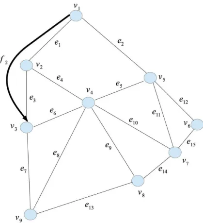
In this chapter, we first present the background information by defining the concepts used throughout this thesis followed by the problem description. Then we provide a sample network depicted in Figure 3.1 to further clarify and illustrate the concepts and problem. It is also the sample network we use to evaluate our proposed models. As a brief summarization, the problem we are solving is planning charging facilities on road networks. To be more exact, the types of charging facility that we study in this thesis are charging stations and dynamic wireless charging pads.

An Origin-Destination (OD) pair is a pair of nodes from the road network

G(V, E) that serves as the origin and destination of an EV route/trip. Origins

VO are nodes that generate traffic flows while destinationsVD are nodes that

attract traffic flows. It is obvious that VO ∈V and VD ∈ V. We denote the

set of all OD pairs as Qand use q as the index.

Traffic flowfq denotes the vehicles traveling on the shortest path between

the OD pair q. Traffic flow is described by the number of vehicles passing a reference point on the shortest path during a given time period which is typically in the unit of vehicles per hour. Traditionally, it is assumed that traffic flows are symmetric in the way that flows between OD pairs (Vi, Vj)

and (Vj, Vi) are the same.

3.1 Extended FRLM

In Chapter 6, we propose an extended Flow Refueling Location model to optimally place charging stations and dynamic wireless charging pads on road networks under a budget constraint. In particular, the budge constraint is specified by fixing the number N of available charging facilities.

(17)

for dynamic wireless charging pads. As discussed in previous chapters, charg-ing stations are to be located at nodes of a road network while dynamic wireless charging pads are to be places along links of a network. Therefore, it is straightforward to see that Vst ⊂ V and Epad ⊂ E from the overall

road network G(V, E)1_{. The candidate location set}_V

st has a special case of Vst =V, which means that all nodes on the network are treated as candidate

location set for charging stations. Similarly, Epad = E means that all links

are treated as candidate locations for dynamic wireless charging pads. The objective of the proposed extended FRLM can then be described as finding a set of nodes V_st∗ ⊂Vst and a set of linksEpad∗ ⊂Epad such that the

maximum amount of traffic flows can be charged. Since the number of nodes that get assigned with charging stations can be represented by Nst = |Vst∗|

and the number of road links that are selected to install dynamic wireless charging pads is depicted by Npad = |Epad∗ |, the budget constraint can be

expressed as N =Nst+Npad.

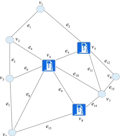
We use the network presented in Figure 3.1 as an example to further clarify the notations and problems described above. The road network has a set of nodes V, where V = {v1, v2,· · · , v9} and a set of links E, where E = {e1, e2,· · · , e15}. The indices are marked next to the corresponding nodes and links. These 9 nodes, V ={v1, v2,· · · , v9} , constitute the set ofVO and VD which means that any node could be an origin as well as a destination.

Therefore, the set Q has 72 OD pairs. Let us take the OD pair of (v1, v3) as

an example. Nodev1 is the origin whilev3 is the destination. Let us assume

this OD pair has an index of 2, thenf2 describes the traffic flow traveling on

the shortest path from v1 tov3.

Let us assume we selectVst =V and Epad=E, then we have 9 candidate

nodes to allocate charging stations and 15 candidate links to place dynamic wireless charging pads. Let us suppose the budget constraint isN = 3 which implies that we are to find 3 locations on the road network to locate either types of the charging facilities. By applying the extended FRLM described in Section 6, the optimal locations are chosen as e4, e5 and e10 due to the

maximal simulated traffic traveling on linkse4,e5 and e10. Then the set Epad∗

contains links e4, e5 and e10, i.e. Epad∗ = {e4, e5, e10} and Vst = ∅ since no

charging stations are placed on the network.

(18)

Figure 3.1: A sample network with 9 nodes and 15 links. Numbers next to nodes are their corresponding indices.

3.2 2-stage planning process for charging stations

In Chapter 7, we propose a 2-stage planning process to solve the charging station planning problem by addressing two questions: 1) where to place the charging stations, and 2) how many charging servers should we place for each charging station.

The goals of the 2 stages are listed below separately:

1. For the first stage, the objective is to determine the optimal locations for allocating charging stations given a fixed number of stations Nst

due to cost constraint. This stage can be seen as special scenario of the problem discussed in the previous section, we adopt the same set of notations for consistency.

Since we only focus on selecting candidate nodes from the road network for charging stations, we exclude links as candidate locations. In this

(19)

stage, we would like to find the set of nodes V_st∗ ⊂ Vst such that the

maximum amount of traffic flows can be served with the constraint of |V_st∗|=Nst (we restrict that each candidate location can only have one

charging station).

2. After obtaining the optimal location set V_st∗ for charging stations from the first stage, in the second stage, we focus on determining the optimal number of charging servers to place for each charging station in order to minimize the waiting time of EV drivers across the entire road network. The constraints are the minimum and maximum number of possible charging servers to place for each charging station, as well as the total number of charging servers. The total number of charging servers to allocate across the road network is Nse. In other words, we work on

finding the optimal solution K∗ of which K_v∗_st indicates the number of charging servers to place for a charging station vst ∈ Vst∗. In other

words, P vst∈Vst∗K ∗ vst = Nse. Also, P vst∈/Vst∗ K ∗

vst = 0 which means that

nodes that are not assigned with charging stations do not have any charging servers (i.e., if a charging station exists or is planned, then at least one on charging server is in the charging station).

Again, we use the network, shown in Figure 3.1, to clarify the notations and problems of the 2-stage planning process:

1. For the first stage, we could choose the candidate location set Vst the

same as the set V, i.e., Vst = V, or a subset of V. Let us assume

we select Vst = V. Then we have 9 candidate locations to allocate

charging stations. The goal of this stage is to find the optimal locations for charging stations under the constraint of a fixed number of stations driven by the budget limit city can spend on charging stations. Let us assume we are to find 2 charging locations with Nst = 2 on the road

network G, by applying the model described in Section 7.1, and the optimal locations are chosen as v4 and v8 due to maximal traffic going

through v4 and v8. Then the set Vst∗ contains nodes v4 and v8, i.e., V_st∗ ={v4, v8}.

2. After finding the optimal locations, the goal of the second stage is to optimally allocate the charging servers to the stations at v4 and

(20)

v8. Let us assume Nse = 3, with the implicit restriction that each

charging station has at least one charging server, the problem is to determine whether the charging station at v4 should have 2 charging

servers ofK_v4∗ = 2 and the charging station at v8 has 1 charging server

of K_v8∗ = 1, or should it be the other way around. If we run the model, presented in Section 7.2, then the solution is K_v4∗ = 2 and K_v8∗ = 1, andK∗ ={0,0,0,2,0,0,0,1,0}represents the optimal server allocation plan across the entire road network G.

(21)

CHAPTER 4 RELATED WORK

In this chapter, we review related work on allocating immobile refueling infrastructures. In [22], authors make decision on locations for new charging infrastructure by developing an agent-based decision support system which identifies patterns in residential EV ownership and driving activities. In [23], authors focus on finding optimal charging station locations for EVs in urbanized areas by developing a two-step model. The first step is transferring road information into data points and then clustering the data points into demand clusters. The second step is building an optimization problem given the clusters. In [24], authors formulate a mixed-integer linear programming problem to minimize the construction cost incurred when building stations. The constraints of the optimization problem ensure a minimum amount of flow being served. The Flow Refueling Location Model (FRLM) proposed in [14, 25] is a flow-based location-allocation model, aiming at finding optimal locations for refueling stations. This model has two critical features which are that: 1) it assumes vehicles stop at refueling stations on their preplanned trips instead of making a single purpose trip to refueling stations and 2) the FRLM takes vehicle’s driving range into consideration which is one crucial factor of EVs.

Another category of the refueling facility planning problem [26] features the queueing issue of vehicles at refueling facilities. This category of problems claims that optimal locations should not just minimize or constrain distances from a demand node to a server node, they should also consider the delay caused by a queue at the refueling facilities. This is an important issue to in-clude when a limited number of infrastructures is available and long refueling times are required, especially in a much more stochastic environment.

In [27], authors develop a simulation-optimization model that determines the optimal locations for electric vehicle chargers to maximize their use by privately owned electric vehicles. Authors use simulation to evaluate the

(22)

deterministic multiple-server delay and level of service. It is shown that although the optimal location is sensitive to the specific optimization crite-rion considered, overall service levels are less sensitive to the optimization strategy.

Approximations for the multiple server delay evaluation are studied in several papers. In [28], author studies the approximation and extended the approximation to M/D/c queues with deterministic service times. In [29], au-thors generalize the approximation to M/G/c queues. In [30], auau-thors study the facility allocation problem with the objective of minimizing customers’ total traveling cost and waiting cost. One critical assumption for their pro-posed model is that each facility only has one server with exponential service times. In [31] authors study the multiple server allocation problem which generalizes the model in [30] by allowing more than one server. Authors pro-pose a model that accounts for queues at the server nodes, assuming demand is allocated to the closest server node. The multiple server allocation prob-lem can be solved using a greedy algorithm to incrementally assign servers, as has been demonstrated in the queueing network literature. The Multiple Server Allocation model, proposed in [31], is designed to minimize the sum of the travel time and the average time spent at the server by allowing more than one servers at each facility.

(23)

CHAPTER 5 REVIEW OF FRLM

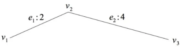
In this chapter, we review the original Flow Refueling Location Model (FRLM). The FRLM is a flow-based model which treats serving demands of road net-works as traffic flows with various OD pairs. FRLM applies a critical concept, combination, which is first introduced in [14]. A candidate combination is defined as a set of candidate locations to locate refueling facilities. The refu-eling facilities discussed in [14] are hydrogen stations and they are assigned to nodes. We use Figure 5.1 to illustrate some examples of combination. Number two and four indicate the length of corresponding links.

Given the short path in Figure 5.1 with values representing length of the corresponding link, if we only allocate stations to nodes, then the follow-ing subsets of nodes constitute all candidate combinations: {v1}, {v2}, {v3},

{v1,v2}, {v1,v3}, {v2,v3}, {v1,v2,v3}. Candidate combination {v1} means a

station is assigned to node v1 only. Candidate combination {v1,v2,v3}

indi-cates that all nodes on the path are assigned with stations.

Each candidate combination is either eligible or ineligible in terms of a specified OD pair. An eligible combination refers to a combination that can refuel vehicles driving a round trip between the origin and the destination without running out of fuel [14]. Otherwise, the candidate combination is ineligible.

We make the following assumptions about EV battery status before or after charging:

(24)

• Let us assume that vehicle’s driving range is 5 units when fully refueled. In other words, the full fuel range is 5.

• A vehicle gets fully refueled after passing a refueling station.

• A vehicle’s starting fuel range is full fuel range if a refueling station is located at the origin of its trip. Otherwise, its starting fuel range is half the full fuel range.

In order to test if a candidate combination is eligible, we need to consider the vehicle’s driving range. For example, in Figure 5.1, if we assume the EV’s full battery range is 5, i.e., an EV with full battery can move a distance of 5 units without charging, then candidate combination {v2} cannot refuel

the OD pair (v1,v3), because the distance for a vehicle to drive from node v2

to node v3 then back to v2 is 2∗4 = 8, which is longer than the EV’s full

battery range of 5.

Now we move on to the details of the FRLM. The FRLM consists of two major steps:

1. Generate and record all eligible combinations for all OD pairs on the study road network.

2. Given the combinations generated by the first step, build an optimiza-tion problem to select combinaoptimiza-tion(s) to achieve a prefixed goal. Detailed description of the first step can be found in [14], where an al-gorithm was developed. Since we will describe its extension in more detail in Chapter 6, we do not repeat it here. Briefly, the first step outputs two matrices {ahp} and {bqh}, which are explained as follows:

• Matrix {ahp} is used to store configuration of each combination. Each

row of matrix {ahp}indicates a distinct combination and each column

represents a candidate location for assigning refueling facilities. Matrix entryahp= 1 when a refueling facility is located at locationp, otherwise

0.

Let us assume we are studying a 9 node network, shown in Figure 3.1, then it means we have 9 candidate locations V = {v1, v2,· · · , v9} to

locate refueling facilities. Thus the number of columns of matrix{ahp}

(25)

• Matrix {bqh} is used to keep track of eligibility of each combination in

terms of each OD pair. Each row of matrix{bqh}represents an OD pair

on the network G= (V, E) and each column represents a combination whose configuration is stored in matrix {ahp}. Matrix entry bqh = 1 if

combination h is able to refuel OD pair q, otherwise 0.

Let us use the 9 node network example in Figure 3.1 again. The network has 36 unique OD pairs (72 OD pairs if we include symmetric OD pairs), so {bqh} has 36 rows. And, if using the{ahp}matrix mentioned

above, the number of columns of matrix {bqh} would be the same as

the number of rows of matrix {ahp}which is 9.

After getting matrices{ahp}and{bqh}from the first step, an optimization

problem is built in the second step which is formulated as follows:

maximize Z =X q f_qTxq (5.1) s.t. X h∈H bqhvh ≥xq, ∀q∈Q (5.2) ahpyp ≥ch, ∀h∈H,∀p∈P (5.3) X p∈P yp =N, (5.4) xq, yp, vh ∈ {0,1}, ∀q,∀h,∀p (5.5) where: q = index of OD pairs.

Q = a set of all OD pairs.

fq = traffic flow, in veh/hr, on the shortest path between OD pair q. xq = 1 if flowfq is refueled, otherwise 0.

bqh = 1 if combination h could refuel flowfq, otherwise 0. h = index of combination.

H = a set of all combinations.

ch = 1 if all facilities in combination h are selected to get assigned,

other-wise 0.

p = index of candidate location.

P = a set of all candidate locations.

(26)

combi-nation h, otherwise 0.

yp = 1 if a refueling facility is assigned to candidate location p. N = fixed number of refueling facilities to locate on the network.

The objective of this optimization problem is to maximize the refueled flow volume as described by Equation (5.1). Constraint (5.2) specifies that a flow

fq is considered refueled only when at least one of its eligible combination

is selected. Constraint (5.3) specifies that an eligible combination is consid-ered selected only when all of the facilities required by the combination are actually being assigned with refueling facilities. Constraint (5.4) fixes the total number of refueling facilities to locate on the network. Constraint (5.5) specifies that xq, yp and vh are all binary variables. By restricting xq to be

either zero or one, it makes sure each refueled flow is counted at maximum one time.

(27)

CHAPTER 6 EXTENDED FRLM

In this chapter, we introduce our proposed extended FRLM [1] which aims at finding optimal locations for both charging stations and dynamic charging pads on road networks.

As discussed in Chapter 2, charging stations share the same feature as conventional refueling stations, such as gas stations. Therefore, they are typically assigned to nodes of a road network. On the other hand, dynamic wireless charging pads charge EVs while EVs are driving above them [13] which implies that the number of adjacent charging pads, embedded along the links of a road network, determines the amount of electricity an EV could obtain while traveling on the link. As a conclusion, we assign charging stations to nodes v ∈ V (points of interest) and dynamic wireless charging pads to links e∈E of road networks G= (V, E).

In contrast to the combinations discussed in Chapter 5, we consider candi-date combinations including links for the purpose of locating dynamic wire-less charging pads. To better illustrate the differences, we revisit the short path example described in Figure 5.1.

All candidate combinations including both nodes and links are listed under the following three situation:

• If we only locate charging stations, then the candidate combinations are the same with the combinations discussed in Chapter 5.

• If we only locate dynamic wireless charging pads, then the following subset of links constitute all candidate combinations{e1},{e2},{e1,e2}.

Candidate combination {e1} means that a charging pad is assigned to

link e1.

• If we consider both charging stations and dynamic wireless charging pads, then candidate combinations are all possible combinations of two

(28)

candidate combinations, each from the above two separate lists. Note that we exclude the combinations where we assign both dynamic wireless charging pads to a link and charging station to one of its end-point. For example, combination {v1,e1}is not considered a candidate

combination since nodev1 is assigned with a charging station and is on

linke1, which has a dynamic wireless charging pad. In contrast,

combi-nation {v1,e2}is a valid candidate combination. The reason of setting

this criteria is to decrease the size of the set of candidate combinations. The intuition behind this is the maximum flow refueling objective will not be achieved by having overlapping charging facilities since spread-ing them would have a higher chance of servspread-ing more flows. Thus, we suspect that, even though all candidate combinations including those with overlapping facilities were fed into the optimization solver, they should be eliminated eventually.Therefore, we are pre-excluding these combinations to reduce the burden of optimization solver.

As we have discussed in Chapter 5, to test the eligibility of candidate combinations, we need to consider the driving range of EVs. Since an EV can be charged while moving above the dynamic wireless charging pads, we assume that the State-of-Charge (SoC) of EV’s battery remains the same while moving on links which are equipped with dynamic wireless charging pads. In other words, there is no battery consumption as long as an EV drives on a link which has dynamic wireless charging pads.

This is in fact a conservative assumption since driving above charging pads actually increases remaining energy of an EV. For example, the energy consumption rate of Nissan Leaf 2011 model is 34kW [32]. As discussed in [17, 18, 19], charging pads are capable of achieving 37kW to 51kW energy transfer. It proves that driving above charging pad increases SOC level.

We pick one candidate combination from each situation discussed above to test their eligibility as an illustration.

• Candidate combination {v1} from the first situation is not an eligible

combination. This is proved in Chapter 5 already.

• Candidate combination{e1}from the second situation is not an eligible

combination since the starting remaining fuel range of EV is 2.5 (since there is no charging station at node v1 and it is assumed that EV’s

(29)

starting fuel range is half the full fuel range when its origin has no charging station which is stated in Chapter 5). The EV cannot make round trip from node v2 to v3 with remaining fuel range of 2.5.

• Candidate combination {v1,e2} from the third situation is an eligible

combination since an EV gets fully charged at node v1 (since node v1

has a charging station) and it can make a round trip from node v1 to

node v2 along with the fact that no energy consumption on the round

trip from node v2 tov3.

The extended FRLM shares the same two steps as introduced in Chapter 5: 1) generate eligible combinations for all OD pairs; and 2) formulate an optimization problem to find optimal solutions. However, since the extended FRLM considers locating facilities to both links and nodes of a road network, the algorithm and model applied to these two steps are adjusted accordingly. Details about these two steps are introduced in the two following sections.

6.1 Eligible combination generation

An algorithm is developed in [14] to check eligibilities of different combina-tions that consists of nodes. In this section, since we consider combinacombina-tions with links as well, we extend the algorithm so that it takes both nodes and links into consideration in order to model charging station and dynamic wire-less charging pad placement.

If we consider all possible combinations of links and nodes, then the number of candidate combinations explodes, and results in a large decision space for the optimization problem, formulated in the second step. Instead of treating each single link as a candidate site to assign dynamic wireless charging pads, we treat each OD pair as an entity to assign charging pads.

For example, if there is only one traffic flow in Figure 5.1, which has EVs travel from origin node v1 to destination node v3, we do not consider

assigning dynamic wireless charging pads to either link e1 or link e2 but to

assign charging pads to the entire link of (v1, v3) (which consists of e1 and e2). As long as the OD pair (v1,v3) is chosen to assign with dynamic wireless charging pads, link e1 and link e2 will both get assigned. On the other hand, if there are two distinct traffic flows one has OD pair of node v1 and node v3

(30)

and the other one with OD pair of node v1 and node v2, then when choosing

the optimal locations for allocating dynamic wireless charging pads, we need to consider 2 different situations that: 1) the OD pair of (v1,v3) is selected

to embed dynamic wireless charging pads, or 2) only OD pair of (v1,v2) is

selected which means linke1 is assigned with dynamic wireless charging pads

while link e2 does not get assigned with any pads. Note that we do not

need to consider the situation when both OD pairs of (v1,v2) and (v1,v3) are

selected since choosing OD pair of (v1,v3) alone would result in OD pair of

(v1,v2) to be assigned with dynamic wireless charging pads automatically. In other words, assigning charging pads to link (v1,v3) cover linke1by definition. Inputs of the algorithm are the network topology and driving range of EV, and outputs are two matrices {ahp} and{bqh}which have the same meaning

as in Chapter 5, with a slight difference on the number of columns of matrix {ahp}.

Revisit the short path example in Figure 5.1. According to Chapter 5, matrix {ahp} has 3 columns since there are 3 candidate locations to place

charging stations. However, in our case, assuming we select 2 candidate OD pairs to assign dynamic wireless charging pads and 3 candidate nodes to place charging stations, the number of columns of matrix {ahp} would then

become 5.

Next we introduce the algorithm to generate matrix {ahp} as follows: Step 1: initialization. Generate shortest paths for all OD pairs and store their corresponding nodes and links. Keep a list of all OD pairs Q.

Step 2: select OD pairs as candidate ODs to assign dynamic wireless charging pads. Given a network with more than one OD pair, select a subset of OD pairs,R, to be candidate ODs. Normally, one good cri-teria for picking candidate ODs is choosing the ones with the top traffic flow volumes so that the heavy traffic flows have a higher priority to be serviced.

Step 3: initialize matrix {ahp} as an empty matrix with a number

of n columns where n is the summation of the number of

candi-date nodes and the number of candicandi-date paths.

(31)

1. Begin with the first OD pairq on the list of Q.

2. List all candidate combinations when assigning charging stations only. 3. If q is in listR, list the combinations of q assigned with charging pads only and the combinations of assigning both charging pads and charing stations. Else, skip this step.

4. Repeat the above two steps until candidate combinations are generated for all OD pairs in Q.

5. Record all combinations in matrix {ahp}.

Step 5: check eligibility for all combinations by discussing if EV could complete trips with limitation of its driving range.

1. Initialize matrix bqh with entries all zero.

2. Begin with the first candidate combination h and the first OD pair q. Generate a round trip qr for OD pair q.

3. If any links of trip qr in combination h is assigned with charging pad,

update the energy cost of corresponding links to zero. This is based on the assumption that SOC of EV remains the same while driving above charging pads.

4. If a charging station is located at the origin of pathqr, set the starting

fuel range as full fuel range. Otherwise, set it as half of the full fuel range.

5. Check if combination h is an eligible combination for OD pairq. • Start from origin node and move to the next node on the round

trip path qr. Update the remaining fuel range by subtracting the

fuel cost from the remaining fuel range at previous node.

• If the remaining fuel range is negative. We reached the conclusion that the combinationhis not able to refuel path q. Leave bqh = 0

as initialized. Go check the next combination for pathq.

(32)

If the current node is destination node of path q and there is a charging station at the destination node, then combination h can refuel OD pair q. Set bqh = 1 and go check the next combination.

If the current node is the origin node, then the EV is able to make a round trip without running out of energy. This is an eligible combination. Set bqh = 1 and go check the next combination.

If the current node has a charging station, update the remaining fuel range to full fuel range.

• Move to the next node and repeat the same procedures until the round trip is checked.

6. Repeat the above steps until the eligibility of all combinations have been evaluated for all OD pairs.

Step 6: for each OD pair q, remove combinations which are su-persets of any other remaining combination. For example, in Figure 5.1, if combinations {v1,v2,v3}and{v1,v3}for OD pair of (v1,v3) are both

eli-gible, we remove combination {v1,v2,v3} since it is a superset of combination

{v1,v3}. We prefer the smaller combination due to the fact that it requires fewer charging facilities.

6.2 Optimization problem formulation

After generating matrices {ahp} and {bqh}, The allocation problem is

for-mulated into an optimization problem with the objective of maximizing the refueled volume of traffic flows described by (6.1):

(33)

maximizeZ =X q f_qTxq (6.1) s.t. X h∈H bqhvh ≥xq, ∀q ∈Q (6.2) ahpyp ≥ch, ∀h∈H,∀p∈P (6.3) X p∈P yp =N, (6.4) ypn +ypr ≤1, ∀pn∈pr,∀pn ∈P,∀pr ∈P (6.5) xq, yp, ch ∈ {0,1}, ∀q,∀h,∀p (6.6)

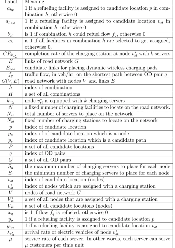
Notations of the model and their meanings could be found in Table 6.1. Constraint (6.2) specifies that a flow fq is considered refueled only when at

least one of its eligible combination is selected. Constraint (6.3) specifies that an eligible combination is considered selected only when all of the facilities, required by the combination, are actually being assigned with refueling facili-ties. Constraint (6.4) fixes the total number of refueling facilities to locate on the network. Constraint (6.5) means that no overlapping of charging station and charging pad is allowed. This is achieved by restricting the number of facilities a node could be assigned is at maximum one. In other words, when charging pad is assigned to one candidate path, none of the nodes on this path could get assigned with charging station anymore.

Let us use the 9-node network in Figure 3.1 as an example limiting the number of charging facilities to place on the road network to 3 with pre-generated traffic flows. Apply the optimization model discussed above, as shown in Figure 6.1, the model chooses to place 3 charging stations on the network at nodes v4, v5 and v8 and no dynamic wireless charging pads are

selected. The traffic flows that could be charged on the road network are the ones with OD pairs of (v4, v5), (v4, v8) and (v5, v8).

Note that this model helps choosing optimal locations for both charging stations and dynamic wireless charging pads, it can be modified to allocate either charing stations or dynamic wireless charging pads only. We present the modified model in Chapter 7.

(34)

Label Meaning

ahp 1 if a refueling facility is assigned to candidate locationpin

com-bination h, otherwise 0

ahvst 1 if a refueling facility is assigned to candidate location vst in

combination h, otherwise 0

bqh is 1 if combinationh could refuel flow fq, otherwise 0

ch is 1 if all facilities in combination h are selected to get assigned,

otherwise 0.

CRkv_st∗ completion rate of the charging station at nodev

∗

st withk servers E links of road networkG

Epad candidate links for placing dynamic wireless charging pads fq traffic flow, in veh/hr, on the shortest path between OD pair q G(V, E) road network with nodes V and links E

h index of combination

H a set of all combinations

kv∗

st nodev

∗

st is equipped with k charging servers

N a fixed number of charging facilities to locate on the road network.

Nse total number of servers to place on the network

Nst fixed number of charging stations to locate on the network p index of candidate location

pn index of of candidate location which is a node

pr index of candidate location which is a candidate path P a set of all candidate locations

q index of OD pairs

Q a set of all OD pairs

Su the maximum number of charging servers to place for each node Sl the minimum number of charging servers to place for each node vst index of candidate location (nodes)

v_st∗ index of nodes which are assigned with a charging station

V nodes of road network G

V_st∗ a set of all nodes that are assigned with a charging station

Vst a set of all candidate locations (nodes) xq is 1 if flow fq is refueled, otherwise 0

yp 1 if a refueling facility is assigned to candidate locationp yvst 1 if a refueling facility is assigned to candidate locationvst

λvst∗ arrival rate of electric vehicles of nodev

∗

st

µ service rate of each server. In other words, each server can serve

µcustomers per time unit

(35)

Figure 6.1: Example of placement of 3 charging facilities on a road network with 9 nodes.

(36)

CHAPTER 7 THE 2-STAGE PLANNING PROCESS

In this chapter, we introduce our proposed 2-stage planning method for charg-ing facilities [2]. More specifically,

1. the first stage applies the modified Extended FRLM (FRLM) model which is based on the FRLM proposed in [14] to help finding the optimal locations for charging facilities so that the maximum amount the traffic flows could be refueled under a budget constraint,

2. in the second stage, we formulate an optimization problem with the goal of finding the optimal configuration plan for charging stations, i.e., optimal number of charging servers per charging station, so that the charging completion rate of the whole system is maximized.

7.1 First stage

The allocation problem is formulated into an optimization problem with the objective of maximizing the volume of refueled traffic flows described by (7.1).

maximizeZ1 =X q f_qTxq (7.1) s.t. X h∈H bqhch ≥xq, ∀q∈Q (7.2) ahvstyvst ≥ch, ∀h∈H,∀vst ∈Vst (7.3) X vst∈Vst yvst =Nst, (7.4) xq, yvst, ch ∈ {0,1}, ∀q,∀h,∀vst (7.5)

(37)

optimization problem from Chapter 6 except for vst, Vst, ahvst, yvst and Nst.

The meaning of these notations could be found in Table 6.1.

Constraint (7.2) specifies that a flowfqis considered charged only when at

least one of its eligible combinations is selected. Since charging stations are the only charging facilities being considered and they are to be placed only at nodes of road networks, candidate combinations only consists of nodes of road networks and has the same definition as in Chapter 5. Also, the definition of eligible combination of a traffic flow f can be found in Chapter 5 which is defined as a combination, from the candidate combinations, that could ensure EVs to make a round-trip between the origin and destination of flow f. Constraint (7.3) specifies that an eligible combination is considered selected only when all of the nodes of the road network required by the combination are actually being assigned with charging stations. Constraint (7.4) fixes the total number of charging stations a city can afford to purchase. Constraint (7.5) specifies that xq, yvst and ch are binary variables.

7.2 Second stage

After obtaining the optimal location setV_st∗ of nodes (i.e. points of interests) to place charging stations from the first stage, we formulate the configuration planning process of charging server per station as an optimization problem below.

The objective is to maximize the EV’s charging completion rateCR, which depends on the number of serverskat each charging stationv_st∗ ∈V_st∗, arriving rate λ and service rate µ of EVs at each charging station v_st∗ ∈ V_st∗, for all charging stations, on the city road network, as described by Equation (7.6). Notations of the model and their meanings could be found in Table 6.1.

maximizeZ2 = X vst∗∈Vst∗ CRkv∗ st (λv∗ st, µ) (7.6) s.t. X v∗_st∈V_st∗ kv∗ st =Nse (7.7) kv∗st ≤Su, ∀v ∗ st ∈V ∗ st (7.8) kv∗ st ≥Sl, ∀v ∗ st ∈V ∗ st (7.9)

(38)

Constraint (7.7) specifies that the total number of charging servers kv∗

st to

place across the network isNse. Constraint (7.8) and Constraint (7.9) specify

the maximum and minimum number of servers kv∗

st to place for each node

(39)

CHAPTER 8 EVALUATION

In this chapter, we evaluate our proposed extended FRLM and the 2-stage planning process separately in the following section.

8.1 Extended FRLM

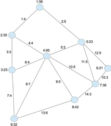
In this section, we evaluate the extended FRLM on the network, shown in Figure 8.1. We use A:B notation in the figure, where A represents the index of the corresponding link eA ∈E or node vA ∈V and B denotes the weight

of the node (i.e. popularity of the node or importance of the location) of the city road network, G= (V, E), or length of the link.

We assign each node with a weight and each link with a length. The length of links describes the distance between two points on the road network G. The weight of each point describes the popularity of each node, i.e., high weight means high popularity. High popularity of a location results from, for example, being a tourist attraction or being a shopping mall.

The feature of this network is that Node 4 is the center node which has the highest weight while rest of the nodes share similar weights and the weights are lower than the weight of Node 4. According to explanations before, Node 4 attracts most of the traffic flows traveling to the center.

One real life example of this type of network is the city Berlin of Germany. Berlin is grouped into six districts with district Mitte in the center and the other five surrounding it. The center district Mitte attracts and generates large volumes of traffic flows into the center. Therefore, studying the network in Figure 8.1 helps us to have a better understanding on how the charging facilities should be located for such center-formed networks and later apply the model to similar cities.

(40)

Figure 8.1: A sample network with 9 nodes, where A:B indicates that node (link) A has weight (length) B.

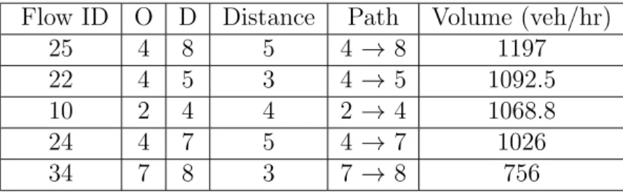
listed in Table 8.1 as examples. As we can see from Table 8.1, flows traveling from the center Node 4 to other surrounding nodes have the top flow volumes which corresponds to the fact that center Node 4 attracts and generates most of the flows.

When testing the extended FRLM model discussed in Section 6, we set the necessary variables as follows:

• number of facilities Nst equals 3.

• Number of candidate paths equals 5. • Full fuel range of EV is 5 unit

We pick candidate paths based on flow volumes in decreasing order. There-fore, Flow 25, Flow 22, Flow 10, Flow 24, and Flow 34 are candidate paths to assign charging pads which are listed in Table 8.1.

(41)

Table 8.1: Top flows of the 9 node network Flow ID O D Distance Path Volume (veh/hr)

25 4 8 5 4→ 8 1197

22 4 5 3 4→ 5 1092.5

10 2 4 4 2→ 4 1068.8

24 4 7 5 4→ 7 1026

34 7 8 3 7→ 8 756

Table 8.2: Served flows with Link 4, Link 5, and Link 10 assigned with charging pads.

Flow ID O D Distance Path Volume (veh/hr)

10 2 4 4 2→ 4 1068.8

11 2 5 7 2 → 4→ 5 147.86

13 2 7 9 2 → 4→ 7 180

22 4 5 3 4→ 5 1092.5

24 4 7 5 4→ 7 1026

Note that the traffic flows in the table represent the general traffic flows of registered vehicles, namely EVs and conventional vehicles. Since the number of EVs on the road network are proportional to all the registered vehicles (i.e. the general traffic flows), serving the maximum amount of general traffic flows helps to achieve the goal of serving the maximum amount of EVs. In order to calculate the number of EVs, out of the general traffic flows, that could be charged, we need to obtain the EV market share of the studied road network and multiply the percentage share with the volumes of general flows that could be served. Note that, one special situation, with the EV market share of 100%, the volumes of traffic flows presented in Table 8.1 is also the number of EVs that could be charged.

Apply the model from Chapter 6 and the optimal solution is to locate charging pads and charging pads only on the network. The configuration is assigning charging pads to Flow 10, Flow 22, and Flow 24. The corresponding links are Link 4, Link 5, and Link 10. The total amount of flows being served is 3515.1 (veh/hr). Details of charged flows by this combination are listed in Table 8.2.

Since we are locating 3 charging facilities on the network, the possible situations of charging pads and charging stations are:

(42)

Table 8.3: Maximum flow served under various situations # pad # station Configuration Volume (veh/hr)

3 0 Link 4, Link 5, Link 10 3515.1

2 1 Link 4, Link 5, Node 1 2309.1

1 2 Node 1, Node 2, Link 5 2726.9

0 3 Node 1, Node 2, Node 4 1692.2

• locate 2 charging pads and 1 charging station, • locate 1 charging pad and 2 charging stations, • locate 3 charging stations.

Next, we compare the performance of the optimal solutions each from the above situations in Table 8.3:

As we can see from Table 8.3, locating 3 charging pads on the network is doubling the amount of general traffic flows when compared with flows being charged by locating 3 charging stations only.

Next, we compare the charging time, i.e., contact time, when placing charg-ing stations and chargcharg-ing pads. Let us suppose we study EV model of Nissan Leaf driving between OD pair Node 2 and Node 7. The battery capacity of Nissan Leaf is 24kW h and its driving range is about 70 miles [33] which corresponds to the 5 unit of full fuel range we assumed previously. Scale the distance accordingly, then the distance of the round trip between this OD pair is 126 miles. Also, let us assume the speed limit is 70mile/hr meaning without stops, it takes 1.8 hours to complete the trip. If (e4, e10) are equipped

with wireless dynamic charging pads, since EVs do not need to stop in the middle of the trip, the amount of time required to complete the trip is also 1.8 hours.

On the other hand, let us assume slow charging servers with 3.6kW are installed at charging stations, which leads to the result that, to complete the trip, an EV needs to charge at least twice and it takes about 7.6 hours to charge the EV. Plus the 1.8 hours to travel the distance, it takes 9.4 hours in total to complete the trip.

Therefore, driving between the OD pair (v2, v7) requires at least 5 times of

charging time if charged at charging stations instead of driving over charging pads (e4, e10, e10, e4), which shows that EV drivers would benefit from

(43)

1 2 3 4 5 6 7 8 9 1000 2000 3000 4000 5000 6000 7000 8000 9000 10000 11000

Refueled flow volume given various number of facilities

number of facilities

refueled flow volume (veh/hr)

Figure 8.2: Served flow volume given various number of facilities. charging time. Also, assigning charging pads to roads could be considered for those who have high traffic volumes or those who are required to have shorter travel time and higher efficiency.

Next, we show the effect of locating different number of facilities on the charged traffic flow volumes.

As shown in Figure 8.2, the total amount of traffic flows being served increased with the number of charging facilities to locate. This meets our expectation since increasing accessibility of charging facilities by EVs enables EVs to travel longer distances. However, increasing the number of facilities on a network raises the building and management cost which is normally a limitation.

Given the fact that discussions on comparison between the costs on build-ing and managbuild-ing chargbuild-ing stations and chargbuild-ing pads are not available, so we restrict the number of charging facilities to control budget.

(44)

O D Distance Path Volume (veh/hr)

4 5 3 4 → 5 1092.5

4 8 5 4 → 8 1197

5 8 8 5 →4 → 8 181.1

Table 8.4: Charged flows with Node 4, Node 5 and Node 8 assigned with charging stations.

8.2 2-stage planning process

In this section, we evaluate the 2-stage allocation model on the same sample network which is shown in Figure 8.1.

8.2.1 First stage

We first test the 2-stage planning model starting by finding the optimal locations for EV charging stations. We set the essential variables as follows:

• The total number of charging stations to allocate is 3, i.e. Nst = 3.

• The full battery range of EV is 5 unit. Take a fully charged EV traveling from Node 1 to Node 2 as an example. Since the starting battery status of an EV is 5 and the length of Link 1 is 4, the EV is able to travel from Node 1 to Node 2 without charging. However, if the driver is traveling a round trip between Node 1 and Node 2 and would like to drive back to Node 1, the remained 1 unit of battery would not be suffice and charging is required.

We apply the model from Section 7.1 and the model outputs the opti-mal locations for charging stations as Node 4, Node 5 and Node 8, which means V_st∗ = {v4, v5, v8}. The total amount of traffic flow being charged is 2470.6(veh/hr). Detailed charged traffic flows information is listed in Table 8.4.

8.2.2 Second stage

Next, we proceed to the second stage of the planning process which is deter-mining the optimal number of charging servers to allocate for each charging

(45)

station. We use SimPy [34] to simulate the queueing process of EVs at charg-ing stations. In the mean time, we make a couple of assumptions which are listed below:

• we assume the traffic flows stays constant during the day. In other words, we do not consider peak hour affects on traffic flows (to be considered in future work),

• we assume that electric vehicles arrive to charging stations following poisson distribution,

• to simulate the charging preference and behavior of EV drivers more practically, instead of assuming all EV drivers prefer to charge to full battery capacity, we assume that 50% of EV drivers are cautious drivers and would like to get fully charged every time they go into a charging station. However, the other 50% of EV drivers are more concerned about the long charging times, so they are only charging to the battery level that is enough to support them to travel to the next charging station.

Note that the amount of electricity EV drivers request determines the service rate of charging servers, i.e., drivers with their EVs charge to full battery takes more time than those drivers who request less electricity given the same charging server.

We consider fast chargers at charging stations which have a maximum of 50kWh output and the service rate of the fast chargers is 2.08 EV/hr. The duration of our simulation is one day (i.e., 24 hours) and we assume the EV market share is 0.3% (i.e., 3 EVs out of 1000 registered vehicles). According to [35], in California, there are 3 EVs per 1000 registered vehicles and California is the state with the highest EV market share in the United States.

In Figure 8.3, we show the relationship between the completion rate and the number of servers for each charging station. The EV market share plays an import role in determining the number of servers for each charging station since higher EV shares indicate higher numbers of EVs arriving at charging stations which results in longer waiting queues given the same number of charging servers at charging stations. To maintain a satisfactory completion

(46)

Figure 8.3: Completion rate (%) with various number of servers). rate, a increasing number of charging servers are required to be installed in order to accommodate the increasing number of incoming EVs.

Again, completion rate is defined as the division between the number of charged EVs and the number of arrived EVs. As we can see, with the low EV market share, it is easy to achieve almost 100% completion rate for all these 3 charging stations.

After getting the completion rate of each charging station under various number of charging servers CRk_vst(λvst, µ), we find the optimal number of

servers to allocate for each charging station by constructing the optimization problem discussed in Section 7.2. We set the parameters of the optimization as follows:

• the total number of servers to deploy is Nse= 10,

• the minimum number of servers for each station is Sl = 2,

• the maximum number of servers for each station is Su = 10.

Solving the optimization problem, the solution shows that it would be optimal to place 6 servers at Node 4, 2 servers at Node 5 and 2 servers

(47)

Node index # Servers Traffic flows (veh/hr) Completion Rate (%)

4 6 2465.6 99.54

5 2 1273.6 100

8 2 1378.1 98.98

Table 8.5: Charging station configuration.

Figure 8.4: Completion rate under various EV market shares (%). at Node 8. Therefore, as a final result, given 3 charging stations and 10 charging servers, the 2-stage planning process outputs the optimal planning configuration as presented in Table 8.5. And this configuration gives an averaged completion rate of 99.51% across the 3 charging stations which is quite satisfactory.

Even though the model works perfectly well with the current low EV mar-ket share, we would like to investigate its performance further given higher market shares. We additionally tested our model against market shares rang-ing from 1% to 50% and the result is presented in Figure 8.4.

Next, we compare the averaged completion rates obtained under various market shares. In order to obtain the completion rates, we only need to change the arrival rates of EVs at charging stations to reflect different market shares. Since higher EV market shares implies more EVs on the road network,

(48)

Figure 8.5: Number of servers needed to achieve a 75% completion rate under various EV market shares (%).

arrival rates increase accordingly. The specific values of arrival rate can be calculated from the traffic flow volumes.

With market share increased from 0.3% to 10%, we see that the comple-tion rate decreases dramatically from 99.51% to 16.6%. And the completion rate drops below 10% with EV market shares higher than 15%. This low completion rate is due to the inevitable long charging time as well as the limited number of charging servers.

We next study the minimum number of server required to achieve an aver-age of 75% of completion rate under various EV market shares and the result is presented in Figure 8.5. The figure shows an almost linear relationship be-tween the EV market share and the number of servers required to sustain a 75% completion rate. Since increasing the market share of EVs results in a linearly increasing number of EVs arriving at charging stations, to maintain a completion rate of 75%, the number of servers (i.e., the service rate of the charging station) needs to increase correspondingly.

Besides the fast charging servers, we also tested the planning model con-sidering chargers with slower power (e.g. 3.6kW) and the completion rate is included in Table 8.6. Note that fast charging stations are stations equipped

(49)

# servers Fast charging station (%) Regular charging station (%)

6 99.79 28.58

9 99.92 34.81

12 99.95 41.78

15 99.98 46.72

Table 8.6: Completion rate comparison between fast and slower charging stations.

with fast chargers while regular charging stations are equipped with slow charging servers which power is 3.6kW. Therefore, fast charging stations have higher service rate compared to regular charging stations.

The completion rates are obtained from the charging station place at Node 4. It is obvious to see that completion rates of deploying these slower chargers are significantly smaller than the completion rates obtained from fast charg-ers. And it is safe to say that the charging speed of the servers plays a critical role in the charging station planning process. It is also straightforward to see because the charging speed of charging servers impact the service rate of a charging server. Therefore, if a charging location is considered to serve EVs similar to conventional gas stations, fast chargers are essential. On the other hand, if a charging location is also serving as a parking spot which allows EVs to park several hours with drivers left for shopping malls or offices, slow chargers are acceptable.