2011
Machine learning methods for omics data
integration
Wengang Zhou
Iowa State UniversityFollow this and additional works at:
https://lib.dr.iastate.edu/etd
Part of the
Electrical and Computer Engineering Commons
This Dissertation is brought to you for free and open access by the Iowa State University Capstones, Theses and Dissertations at Iowa State University Digital Repository. It has been accepted for inclusion in Graduate Theses and Dissertations by an authorized administrator of Iowa State University Digital Repository. For more information, please [email protected].
Recommended Citation
Zhou, Wengang, "Machine learning methods for omics data integration" (2011).Graduate Theses and Dissertations. 12238.
by
Wengang Zhou
A dissertation submitted to the graduate faculty in partial fulfillment of the requirements for the degree of
DOCTOR OF PHILOSOPHY
Major: Bioinformatics and Computational Biology
Program of Study Committee: Julie A. Dickerson, Co-major Professor
Xun Gu, Co-major Professor Guang Song
David Fernandez-Baca Rajeev Arora
Iowa State University Ames, Iowa
2011
DEDICATION
I would like to dedicate this thesis to my parents without whose support I would not have been able to complete this work. They have shown great love and encouragement to let me pursue this degree. I would also like to thank my friends for their loving support during the writing of this work.
TABLE OF CONTENTS LIST OF TABLES . . . vi LIST OF FIGURES . . . ix ACKNOWLEDGEMENTS . . . xiv ABSTRACT . . . xv 1. INTRODUCTION . . . 1
2. STRULOCPRED: STRUCTURE-BASED PROTEIN SUBCELLULAR LOCALISATION PREDICTION USING MULTI-CLASS SUPPORT VEC-TOR MACHINE . . . 4
Abstract . . . 4
Introduction . . . 4
Protein features . . . 6
Multi-class Support Vector Machine . . . 9
Performance measurements . . . 10
Experiment results . . . 11
Data Sets . . . 11
Testing and validation . . . 12
Predicting locations in Arabidopsis . . . 16
StruLocPred server . . . 17
Conclusions and Discussions . . . 18
3. MULTI-LABEL SUBCELLULAR LOCALIZATION PREDICTION BASED ON PROTEIN SEQUENCE AND STRUCTURAL FEATURES . . . 20
Abstract . . . 20
Introduction . . . 20
Protein Features . . . 21
Classifiers Review . . . 22
Support Vector Machine . . . 22
Fuzzy K-Nearest Neighbor . . . 23
Extreme Learning Machine . . . 23
Multi-label Classification . . . 24 Experiment Results . . . 26 Dataset . . . 26 Parameter Setting . . . 27 Evaluation Measurements . . . 28 Performance Comparison . . . 28 MLSubLoc Server . . . 31 Conclusions . . . 33
4. A NOVEL CLASS DEPENDENT FEATURE SELECTION METHOD FOR CANCER BIOMARKER DISCOVERY . . . 35
Abstract . . . 35
Introduction . . . 36
Proposed Methodology . . . 37
General Framework . . . 37
Feature Pre-selection with F-statistic . . . 39
Binary Particle Swarm Optimization (BPSO) . . . 39
Classifiers Review . . . 40
Class Dependent Feature Subset Selection by MRBPSO . . . 41
Class Dependent Multi-category Classification Scheme . . . 43
Experimental Results . . . 45
Pre-selected Features for All Datasets . . . 46
Performance Evaluation . . . 46
Cancer Biomarker Discovery . . . 53
Conclusions . . . 58
5. A CLASSIFICATION BASED METHOD FOR INTEGRATED ANAL-YSIS OF METABOLOMICS AND TRANSCRIPTOMICS DATA . . . . 60
Abstract . . . 60
Introduction . . . 61
Classification-based Integration Framework . . . 62
Sparse Binary Particle Swarm Optimization . . . 63
Classification System Connecting Two Data Sources . . . 65
Permutation Strategy for Selecting Predictive Variables . . . 66
Experiment Results . . . 67
Transcriptomics and Metabolomics Data . . . 67
Prediction Comparison between BPSO and SBPSO . . . 69
Biological Interpretation of Selected Variables . . . 70
Comparison with PCA and NMF Methods . . . 73
Gene-Metabolite Correlation Network . . . 75
Identification of Tissue-specific Genes and Metabolites . . . 76
Conclusions . . . 78
APPENDIX A. A PREDICTED INTERACTOME FOR VITIS VINIFERA BASED ON HOMOLOGY MODELING . . . 82
APPENDIX B. COMPARISON OF GENE REGULATORY NETWORK AND PROTEIN-PROTEIN INTERACTION NETWORK FOR ARA-BIDOPSIS COLD STRESS . . . 90
LIST OF TABLES
2.1 Prediction accuracy comparison for RH2427 dataset using different fea-tures . . . 13 2.2 Comparison with other best prediction methods using different features
for RH2427 . . . 14 2.3 Prediction accuracy comparison results for PK7579 data set . . . 14 2.4 The comparison of performance on the animal independent data set . . 15 3.1 The number of proteins in each location used for binary multi-label
classification . . . 27 3.2 The best parameters found and the corresponding balanced accuracy
(BAC) values for each label in MLSVM using HAAP and SSEC features 27 3.3 The comparison of different binary multi-label methods using SSEC,
HAAP, or their combination as features . . . 29 3.4 CPU time (in seconds) used on the testing dataset for all three methods 29 3.5 933 proteins used for multi-class multi-label classificaiton method . . . 32
4.1 Summarization of eight datasets related to human cancers from mi-croarray experiments used in this work . . . 45 4.2 The number of pre-selected features for each class and their
correspond-ing five fold cross validation classification accuracy uscorrespond-ing selected features 48 4.3 The comparison of classification accuracies for various methods
4.4 The average number of features selected by class-dependent method CDMC/SVM and class-independent method MRBPSO/SVM for five datasets in 50 simulations (or iterations) . . . 51 4.5 The average number of features selected by class-dependent method
CDMC/FKNN and class-independent method MRBPSO/FKNN for five datasets in 50 simulations (or iterations) . . . 51 4.6 Top five most frequent genes and their corresponding frequency (in
parentheses) in each cancer class for five datasets identified by CDMC/SVM 56 4.7 Top five most frequent genes and their corresponding frequency (in
parentheses) in all cancer classes for 9 tumors and 11 tumors identified by CDMC/SVM . . . 57
5.1 The gene expression and metabolite accumulation samples for Ara-bidopsis and their corresponding tissue classification information used in this study. . . 68 5.2 The average prediction accuracies (ACC) and average number of
se-lected variables (SEL) in 30 runs using SBPSO with different numbers of top-rankedN variables selected by F-statistic for the two integration work flows. . . 70 5.3 The number of genes and metabolites selected by S and
BPSO-based (N = 1589) integration methods in the best run and the achieved testing accuracies. . . 71 5.4 The average prediction accuracies (in percentage) in 30 runs for different
k dimensional components using PCA and NMF as feature selection methods under our integration framework. . . 73 5.5 The top-identified tissue-specific biomarker genes for all six tissues and
their involved Gene Ontology biological processes. . . 77 5.6 The top-identified tissue-specific metabolites for all six tissues and their
A.1 The corresponding Arabidopsis orthologs and function descriptions of the top 20 proteins with highest degree . . . 86 A.2 GO Annotation for three sub-networks in the predicted Vitis vinifera
interactome . . . 87 A.3 The number of interacting pairs with the same annotated locations . . 89 B.1 20 known cold response genes from TAIR in the 200 differentially
ex-pressed genes list . . . 92 B.2 Partial list of 46 protein interacting pairs from the same location and
LIST OF FIGURES
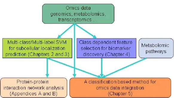
Figure 1.1 The developed methods, the chapters that discuss them, and how they
are related to omics data integration . . . 2
Figure 2.1 Graphical illustration of DPC and HAAP. HAAP looks at both adjacent and gapped amino acid pairs . . . 7
Figure 2.2 Multi-class Support Vector Machine structure . . . 10
Figure 2.3 Grid search for the best parameter values of the RBF kernelγ and SVM penalty factorC. The inner green contour lines show the regions of best performance . . . 12
Figure 2.4 The percentage of each location in Arabidopsis proteome . . . 16
Figure 2.5 Percentage of proteins with known locations in eSLDB matches with predicted locations . . . 17
Figure 2.6 The sample output of prediction results from StruLocPred server . . . 18
Figure 3.1 Extreme Learning Machine Network Structure . . . 24
Figure 3.2 Binary multi-label classification scheme . . . 25
Figure 3.3 The box plot of MF values in 100 runs using SSEC feature . . . 30
Figure 3.4 The box plot of MF values in 100 runs using HAAP feature . . . 31
Figure 3.5 The comparison between binary and multi-class approaches for three multi-label methods using SSEC feature . . . 32
Figure 3.6 The comparison between binary and class schemes for three multi-label methods using HAAP feature . . . 33
Figure 3.7 MLSubLoc server takes a protein sequence as input and allows users to choose any of the three features . . . 34 Figure 3.8 The sample output of MLSubLoc server using SSEC feature and binary
multi-label classification approach . . . 34 Figure 4.1 General framework for proposed class dependent and class independent
feature selection methods.The class dependent method uses different features (genes) for each category that needs to be identified. The class independent method uses the same set of features for all cancer classes. 38 Figure 4.2 The flowchart of class-dependent feature subset selection by MRBPSO 42 Figure 4.3 Class-dependent Multi-category Classification system determines the
class label of the testing sample based on the maximum probability esti-mate of trained models obtained using different class-dependent feature subsets . . . 44 Figure 4.4 The change of the best cross validation accuracies using SVM for
differ-ent feature set sizes in the feature pre-selection step for all eight datasets 47 Figure 4.5 9 Tumors. The number of simulations (or iterations) versus
classifica-tion accuracy for four proposed methods: MRBPSO/SVM, MRBPSO/FKNN, CDMC/SVM, and CDMC/FKNN . . . 50 Figure 4.6 11 Tumors. The number of simulations (or iterations) versus
classifica-tion accuracy. MRBPSO, Maximum Relevance Binary Particle Swarm Optimization; CDMC, Class Dependent Multi-category Classification; SVM, Support Vector Machine; FKNN, Fuzzy K Nearest Neighbor . . 52 Figure 4.7 Leukemia1 (left) and Leukemia2 (right). Class 1 and Class 2 represent
class-dependent genes selected by CDMC/SVM for ALL T-cell, and AML cancers for Leukemia1, and AML, ALL cancers for Leukemia2 re-spectively. For both datasets, Class 3 contains class-independent genes related to all three classes selected by MRBPSO/SVM. . . 53
Figure 4.8 Brain Tumor1 (Left) and Lung Cancer (Right). The class-dependent genes related to each cancer class and common genes involved in any two or three types of cancer identified by CDMC/SVM . . . 54 Figure 4.9 Frequency plots for genes selected by CDMC/SVM in 50 simulations
for all three cancer classes (Class 1 to Class 3) in Leukemia2 dataset. The gene IDs and gene names of top three genes are labeled in black boxes . . . 55 Figure 4.10 Frequency plots for genes selected by CDMC/SVM in 50 simulations
for all five cancer classes (Class 1 to Class 5) in Lung Cancer dataset. Top three most frequent genes are marked in black boxes with their gene IDs and names . . . 58
Figure 5.1 The classification-based framework for integrating omics data includes Gene-to-Metabolite (left), and Metabolite-to-Gene (right) work flows, which identify gene-predictive metabolites and metabolite-predictive genes respectively. . . 63 Figure 5.2 The sigmoid transformation of restricted initial velocities determines
that only a small percentage of variables in the training data can be selected. . . 65 Figure 5.3 The modules using the classification system in the first two steps of the
integration framework include SBPSO module for selecting represen-tative variables and parameters search module for obtaining a trained SVM model. . . 66 Figure 5.4 The comparison of prediction accuracies between BPSO- and
SBPSO-based integration methods for Gene-to-Metabolite work flow. . . 70 Figure 5.5 The comparison of prediction accuracies between BPSO- and
Figure 5.6 The percentage of each subcellular location for the selected 43 genes. Many proteins are predicted to be located in Chloroplasts, Mitochon-dria and Cell Membranes. . . 72 Figure 5.7 The box plot showing the variation of prediction accuracy in 30 runs
for SBPSO (N=1589), PCA (k=20), and NMF (k=30) using top-ranked 1589 genes and all metabolites for Gene-to-Metabolite (left) and Metabolite-to-Gene (right) integration flows. . . 74 Figure 5.8 The overlap of selected genes and metabolites from SBPSO-, PCA- and
NMF-based integration methods. . . 75 Figure 5.9 The percentage of gene-metabolite pairs between selected variables by
SBPSO and all 1589 variables within different correlation ranges. . . . 76 Figure 5.10 Gene and metabolite correlation network for selected variables. Genes
are in light blue ovals and metabolites are in green rectangular shapes. 80 Figure 5.11 The expression profiles of flower-specific genes (left) and accumulation
profiles of flower-specific metabolites (right). The expression in intern-ode and flower tissues is highlighted with a vertical red line . . . 81 Figure A.1 The predicted interactome containing 15242 interactions for grape using
one-way blast . . . 83 Figure A.2 The distribution of nodes degree for all 3682 proteins in the interaction
network . . . 84 Figure A.3 The predicted interactome including 2380 interactions using reciprocal
best blast hits method . . . 85 Figure A.4 The percentage of proteins in each predicted subcellular location in
grape proteome . . . 88 Figure A.5 The proteins from different locations are colored differently for
Figure B.1 Up and down regulated genes in cold stress with 2 fold change and p-value 0.05 cutoff . . . 93 Figure B.2 A meaningful gene regulatory network for 20 Arabidopsis cold response
genes . . . 94 Figure B.3 Cold response protein-protein interaction network visualized by Cytoscape 96
ACKNOWLEDGEMENTS
I would like to take this opportunity to express my thanks to those who helped me with various aspects of conducting research and the writing of this thesis. First and foremost, Dr. Julie A. Dickerson for her guidance, patience and support throughout this research and the writing of this thesis. Her insights and words of encouragement have often inspired me and renewed my hopes for completing my graduate education. I would also like to thank my committee members for their efforts and contributions to this work. I would additionally like to thank collabroators Anne Y. Fennell and Grant Cramer for their advice during my graduate study.
This work was funded by Bioinformatics and Computational Biology program at Iowa State University and the National Science Foundation (NSF) under Grant Number DBI-0604755.
ABSTRACT
High-throughput technologies produce genome-scale transcriptomic and metabolomic (omics) datasets that allow for the system-level studies of complex biological processes. The limitation lies in the small number of samples versus the larger number of features represented in these datasets. Machine learning methods can help integrate these large-scale omics datasets and identify key features from each dataset. A novel class dependent feature selection method inte-grates the F statistic, maximum relevance binary particle swarm optimization (MRBPSO), and class dependent multi-category classification (CDMC) system. A set of highly differentially expressed genes are pre-selected using the F statistic as a filter for each dataset. MRBPSO and CDMC function as a wrapper to select desirable feature subsets for each class and clas-sify the samples using those chosen class-dependent feature subsets. The results indicate that the class-dependent approaches can effectively identify unique biomarkers for each cancer type and improve classification accuracy compared to class independent feature selection meth-ods. The integration of transcriptomics and metabolomics data is based on a classification framework. Compared to principal component analysis and non-negative matrix factorization based integration approaches, our proposed method achieves 20-30% higher prediction accura-cies on Arabidopsis tissue development data. Metabolite-predictive genes and gene-predictive metabolites are selected from transcriptomic and metabolomic data respectively. The con-structed gene-metabolite correlation network can infer the functions of unknown genes and metabolites. Tissue-specific genes and metabolites are identified by the class-dependent fea-ture selection method. Evidence from subcellular locations, gene ontology, and biochemical pathways support the involvement of these entities in different developmental stages and tissues in Arabidopsis.
1. INTRODUCTION
Large-scale omics data such as transcriptomics, proteomics and metabolomics provides cellular activity information in an organism at the levels of genes, proteins and metabolites. Integrating omics data helps understand the cellular responses to enviromental perturbations and developmental events at the system level in plants. The challege lies in the deficiency of computational methods to mine and integrate these data.
The integration of omics data involves the application of various machine learning methods including classification, optimization, and feature selection etc. A variety of annotation infor-mation such as subcellular localization, gene ontology, and metabolic pathways help interpret the integration results.
The purpose of this dissertation is to develop novel machine learning methods for addressing key challenges during the integration of omics datasets. These methods are linked together to provide different biological insights for understanding the complex biological processes. Figure 1.1 illustrates all developed methods and how they are related to the data integration.
This document is organized into five chapters. Each chapter except for the introduction presents a manuscript that is either published in a journal or will be submitted to one for review. Chapter 2 introduces a multi-class support vector machine and three new protein features for predicting subcellular locations. Chapter 3 compares three multi-label classification methods under two schemes for the prediction of multiple subcellular locations for a given protein. The predicted locations are applied to the analyses of protein-protein interaction network, networks comparison, as well as omics data integration.
Chapter 4 proposes a novel class dependent feature selection method integrating F statistic, maximum relevance binary particle swarm optimization, and class dependent multi-category
Figure 1.1 The developed methods, the chapters that discuss them, and how they are related to omics data integration
classification system. Traditional feature selection methods select a set of common features that can differentiate all classes. The proposed method can select a few key features for each class. These features are the candidate biomarkers for different cancer, tissue, or trait. Compared to class independent methods, the proposed method achieves a much higher prediction accuracy as well.
Chapter 5 presents a classification based framework for integrating transcriptomics and metabolomics data. The framework consists of two integration work flows. Gene-predictive metabolites and metabolite-predictive genes are identified from the two flows. A few genes and metabolites specific to each tissue are also discovered by the proposed class dependent feature selection method in Chapter 4. Subcellular locations, gene ontology, and metabolic pathways provide various evidence to show that the identified entities are involved in the different de-velopmental stages and tissues in Arabidopsis. The time delay between gene expression and metabolite accumulation is also observed from the corresponding expression patterns.
interac-tion network and networks comparison analyses. Appendix A builds a protein-protein inter-action network for Vitis vinifera by homology modeling. The functions of three subnetworks are elucidated by GO enrichment analysis. Incorporating subcellular locations increases our confidence for some putative interacting pairs. Appendix B compares the gene regulatory net-work and protein-protein interaction netnet-work for cold stress in Arabidopsis. The results show a significant similarity between the two networks built from different data sources.
2. STRULOCPRED: STRUCTURE-BASED PROTEIN SUBCELLULAR LOCALISATION PREDICTION USING MULTI-CLASS SUPPORT
VECTOR MACHINE
A paper published in International Journal of Data Mining and Bioinformatics Wengang Zhou and Julie A. Dickerson
Abstract
Knowledge of protein subcellular locations can help decipher a proteins biological func-tion. This work proposes new features: sequence-based: Hybrid Amino Acid Pair (HAAP) and two structure-based: Secondary Structural Element Composition (SSEC) and solvent ac-cessibility state frequency. A multi-class Support Vector Machine is developed to predict the locations. Testing on two established data sets yields better prediction accuracies than the best available systems. Comparisons with existing methods show comparable results to ESL-Pred2. When StruLocPred is applied to the entire Arabidopsis proteome, over 77% of proteins with known locations match the prediction results. An implementation of this system is at http://wgzhou.ece. iastate.edu/StruLocPred/.
Introduction
Subcellular localisation is one of the key functional characteristics of proteins. Proteins must be localised to a correct cellular compartment to cooperate for a common physiological function. With the production of a huge amount of raw protein sequence data, the functional annotation of these data is an important task. There are three common experimental ap-proaches for determination of subcellular locations: cell fractionation, electron microscopy and
fluorescence microscopy. Currently, these methods are time-consuming and costly. Compu-tational methods have proved to be an efficient way to accurately determine the subcellular locations from protein sequences.
Numerous methods have been developed to predict the subcellular location using different classifiers and features. Most methods fall into two categories. They are either based on N-terminal sorting signals or Amino Acid Composition (AAC) information. Nakai and Kanehisa (1992) first introduced the use of sorting signals to predict subcellular location. Nielsen et al. (1999) applied neural networks to work on the prediction using signal sequences. Eventually, these individual methods are integrated into a well-known system TargetP (Emanuelsson et al., 2000).
Reinhardt and Hubbard (1998) used a neural network and AAC information to predict four types of subcellular locations for 2427 eukaryotic proteins. Hua and Sun (2001) applied SVM to the same data set and integrated this approach into an online system named SubLoc. Park and Kanehisa (2003) constructed a 7579 proteins data set with 12 types of subcellular locations from Swiss-Prot. Sixty SVM classifiers were trained using AAC and gapped amino acid pairs to predict a protein subcellular location. The results were determined by a majority-voting scheme. An improvement in accuracy was obtained.
Huang and Li (2004) proposed dipeptide information as a feature. They applied a Fuzzy k Nearest Neighbour (FKNN) classifier to the prediction problem. The model was tested on three data sets extracted from Swiss-Prot. There were 12,865 sequences. The data set was further reduced to 7203 and 3572 by removing high similarity sequences. The results showed that dipeptide composition was a useful feature. Bhasin and Raghava (2004) tried several kinds of features including PSI-BLAST information and their combinations. The system, ESLpred, is available online. It used SVMs to classify and was trained using 2427 proteins from Reinhardt. More recently, LOCSVMPSI (Xie et al., 2005) incorporated the position-specific scoring matrix evolutionary information from PSI-BLAST against the NCBI NR database. Su et al. (2007) proposed a hybrid method combining a multi-class SVM classifier based on 1-versus-1 strategy with a structural-homology-based method, which determines the locations from
top-ranked similar proteins with known locations. Another method PairProSVM (Mak et al., 2008) is developed by using PSI-BLAST profiles to obtain pairwise alignment scores as a feature vector.
In this study, we propose three new features for protein subcellular location prediction and investigate the use of a multi-class SVM to predict subcellular locations using these features. Testing on two benchmark data sets RH2427 and PK7579, results are very promising and comparable with the best accuracy in the literature. To compare the performance with latest available methods, we also tested our method on the BaCelLo independent data set. It shows that our method achieves 70.9% total accuracy and performs comparable with the current best method. We further applied these structure-based features to predict the locations for the entire Arabidopsis proteome. The proposed features and modules are implemented as web server named StruLocPred publicly available at http://wgzhou.ece.iastate.edu/StruLocPred/.
Protein features
Five types of features are investigated in this study: AAC, dipeptide composition, HAAP, structural element composition and solvent accessibility state frequency. Amino acid and dipeptide composition have been previously applied in other studies as discussed earlier.
Amino Acid Composition (AAC) Amino Acid Composition is the fraction of each
amino acid in a protein sequence. The fraction of all 20 natural amino acids is calculated using the following equation:
F raction of amino acid= T otal number of amino acid i
T otal number of amino acids in protein (2.1)
Dipeptide Composition (DPC) Dipeptide (amino acid pair) composition gives a fixed
pattern length of 400 (20 20), which represents the occurrence frequency of all amino acid pairs in the protein sequence. This feature encompasses the local order information of amino acids. The fraction of each dipeptide is calculated using the following equation:
F raction of dipeptide(i) = T otal number of dipeptide i
T otal number of dipeptides in the sequence (2.2)
Hybrid Amino Acid Pair (HAAP) This is a new sequence-based feature. It is a
combination of dipeptide and Amino Acid Pairs (AAPs) with a gap. As mentioned earlier for DPC, there are 400 types of AAPs on total. For each pair, we calculate its total number occurring between any two adjacent residues and any two residues with a gap. The fraction can be computed by the following equation:
F raction of AAP (i) = N umber of AAP i in adjacent and with a gap
N umber of AAP s in adjacent and with a gap in protein (2.3)
The dipeptide and HAAP features are illustrated in detail in Figure 2.1. For DPC and HAAP, the total numbers of amino acid pairs in the given protein sequence are L-1 and 2L-3, respectively, as shown in Figure 2.1.
Figure 2.1 Graphical illustration of DPC and HAAP. HAAP looks at both adjacent and gapped amino acid pairs
Secondary structures can indicate the subcellular locations of proteins in some situations. For example, previous work in protein structure studies showed that -helices are frequently observed in inner membrane proteins and -barrels are usually found in outer membrane proteins (Pautsch and Schulz, 1998). It has also been observed that the distribution of surface residues of a protein is correlated with its subcellular environments. Proteins from different locations do show characteristic differences, particularly at the surface, which is directly exposed to the
environment (Andrade et al.,1998). Therefore, we developed two structural features based on the assumption that there is a relationship between protein structures and subcellular locations.
Secondary Structural Element Composition (SSEC) The SSEC represents
fre-quencies of secondary structural elements (H, E, C) for each residue in a given protein sequence. H, E and C represent alpha helix, beta sheet and other structures, respectively. The feature is represented by a 60 (3 ×20) dimensional vector. The frequencies are calculated according to the following formula:
fik= N
k i
L (2.4)
Where i = (H, E, C); fik is the frequency of secondary structural element i occurring
at amino acid k and Nik is the total number of structural elements i found for amino acid
k in the whole protein sequence. L is the length of the protein sequence. The secondary structure prediction is made by PSIPRED 2.5 (Jones, 1999). This system requires calling the PSI-BLAST program. All default parameter values are used. We split the protein sequence into two parts with equal length for the purpose of capturing much structural information to distinguish subcellular locations for different proteins. For each half of the sequence, we obtain a 60 dimensional vector. Therefore, the total length of the feature vector is 120.
Solvent Accessibility State Frequency (SASF) The solvent accessibility contains
two states: buried (B) and exposed (E) for each amino acid. The solvent accessibility state frequency is a 40 (2 ×20) dimensional vector, which gives the frequency information for each state on all the 20 types of amino acids:
fik= N
k i
L (2.5)
Where i= (B, E); fik is the frequency of solvent accessibility state i occurring at amino
acidkandNk
i is the total number of accessibility stateifound for amino acidkin the protein
2002) was used to predict the solvent accessibility states for each residue. Similarly, we split each given protein sequence into two half and achieve an 80 dimensional vector for this feature.
Multi-class Support Vector Machine
The SVM (Vapnik, 1995) is a statistical learning method first proposed by Vapnik. It is based on the theories of VC dimension and structure risk minimisation. For two-class classification problems, SVMs use a non-linear mapping known as a kernel function to map the training data into a higher dimensional feature space, and then construct an optimal separating hyperplane in the higher dimensional space corresponding to a non-linear classifier in the input space. With the kernel functions and the high dimensional space, the hyperplane computation requires solving a quadratic programming problem:
minw,b,ξ 1 2kwk 2+CX i ξi (2.6) s.t.:yi(w·xi+b)≥1−ξi, i= 1,· · ·, m (2.7) C is a tuning parameter that allows the user to control the trade-off between classifying the training samples without error and maximising the margin. Instead of solving this primal problem, it is always a practice to solve its dual problem:
maxα m X i=1 αi− 1 2 m X i,j=1 αiαjyiyjK(xi, xj) (2.8) s.t.: m X i=1 αiyi = 0 (2.9) 0≤αi≤C,∀i (2.10)
αi denotes the Lagrange variable for the ith constraint. K(xi, xj) is the kernel function.
The three commonly used kernel functions include linear kernel, polynomial kernel and Radial Basis Function (RBF) kernel. The RBF kernel with a parameter γ (gamma) is shown in the following equation:
In recent years, multi-class SVMs have been widely used to solve multi-class problems. Most methods divide multi-class problems into several binary classification problems usually based on two strategies: One Versus Rest (OVR) or One Versus One (OVO). We used a multi-class SVM with a probability estimate implemented in LIBSVM 2.85 (Fan et al., 2005). This version SVM is implemented using OVO strategy. The classifier will give a probability estimate belonging to each class for every testing sample. Because of the complexity and non-linearity of subcellular prediction problem, we used RBF kernel in all our experiments. The penalty parameterCand RBF kernel parameterγ need to be tune up for each data set to get the best performance. The general multi-classifier structure is shown in Figure 2.2.
Figure 2.2 Multi-class Support Vector Machine structure
Performance measurements
Three measurements are used to evaluate the performance of classifiers. One is the accuracy, which is the percentage of correctly predicted proteins for each type of subcellular locations. Total accuracy is the percentage of all correctly predicted proteins in the data set. For the first small data set, leave-one-out cross validation is applied to get the accuracy. For the second one, we used 5-fold cross validation. The two accuracies are defined as follows:
Accu(i) = T Pi Ni , T A= Pc i=1T Pi N (2.12)
Where T Pi is the number of correctly predicted proteins in each location i, andNi is the
total number of proteins in location i. N is the total number of proteins in the data set. Matthews Correlation Coefficient (MCC) can overcome the shortcoming of accuracy on unbalanced data. For instance, a classifier may predict the entire training set as positive and not make any prediction on negative samples. In this case, the accuracy will be 1, and the MCC will be 0. Therefore, it is also used as a measure of the prediction performance for each location:
M CC(i) = p T Pi×T Ni−F Pi×F Ni
(T Pi+F Ni)(T Pi+F Pi)(T Ni+F Pi)(T Ni+F Ni)
(2.13) Where F Pi, T Ni and F Ni are false positive, true negative and false negative numbers,
respectively, for subcellular locationi.
Experiment results Data Sets
The RH2427 data set was created (Reinhardt and Hubbard, 1998) by extracting all the protein sequences from Swiss-Prot release 33. It consists of 2427 eukaryotic proteins within four subcellular location categories. There are 1097 nuclear proteins, 684 cytoplasmic proteins, 325 extracellular and 321 mitochondrial proteins.
The PK7579 data set was generated by Park and Kanehisa (2003). It contains 7579 pro-teins in 12 subcellular locations collected from Swiss-Prot release 39. Only those propro-teins with a single subcellular location annotation are selected. There are 671 chloroplast, 1241 cyto-plasmic, 40 cytoskeleton, 114 endoplasmic reticulum, 861 extracellular, 47 Golgi apparatus, 93 lysosomal, 727 mitochondrial, 1932 nuclear, 125 peroxisomal, 1674 plasma membrane and 54 vacuolar proteins in this data set.
The BaCelLo animal independent data set (Pierleoni et al., 2006) contains 1890 proteins in the training data set and 707 proteins in testing data set. As described in Pierleonis paper, proteins in the training data set were extracted from Swiss-Prot until version 41 and the testing data set used the remaining sequences until version 48.
Testing and validation
We first applied the multi-class SVM to predict four types of locations for RH2427 data set. The prediction results with leave-one-out cross validation using different features are listed in Table 2.1. By using leave-one-out cross validation, we leave one protein as test data and use all other proteins as training data each time. In all experiments, we chose to use RBF kernel since it usually performs best for linear inseparable problems. The grid search method is used to find the best parameter value combination of γ and C for SVM from the range of [2−10,2−9,· · ·,210] with step size 21. The search procedure is demonstrated in Figure 2.3. This
procedure is also called model selection. It is always necessary to find the best parameters for each specific data set for machine learning system to have the best performance. The chosen model can be subsequently applied to predict locations for unknown proteins. All results in Table 2.1 are performed by the proposed multi-class SVM and the accuracies are the best accuracies obtained by grid search for SVM parametersγ and C.
Figure 2.3 Grid search for the best parameter values of the RBF kernelγ
and SVM penalty factorC. The inner green contour lines show the regions of best performance
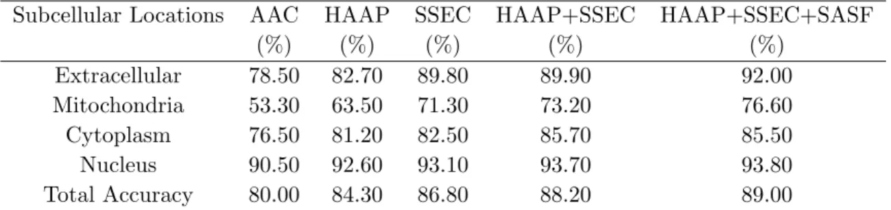
Table 2.1 Prediction accuracy comparison for RH2427 dataset using dif-ferent features
Subcellular Locations AAC HAAP SSEC HAAP+SSEC HAAP+SSEC+SASF
(%) (%) (%) (%) (%) Extracellular 78.50 82.70 89.80 89.90 92.00 Mitochondria 53.30 63.50 71.30 73.20 76.60 Cytoplasm 76.50 81.20 82.50 85.70 85.50 Nucleus 90.50 92.60 93.10 93.70 93.80 Total Accuracy 80.00 84.30 86.80 88.20 89.00
Groups of features usually perform better than single features because the combined fea-tures contain more information about subcellular location. Each feature might be a weak predictor and contribute only a small portion to the prediction. In our study, we combine two structure-based features SSEC (120D) and SASF (80D) with one sequence-based feature HAAP (400D). The total feature vector length is 600 dimensions. The best accuracy, 89.0%, is achieved when combining those three features. The corresponding best SVM parameter value combination is C = 16 and γ = 64. By using the same classifier, we can find that the accuracy obtained from the assembled features is about 9% higher than using conventional AAC alone. The accuracy is 2.5% higher using SSEC than using HAAP. This demonstrates the effectiveness of these proposed structural features.
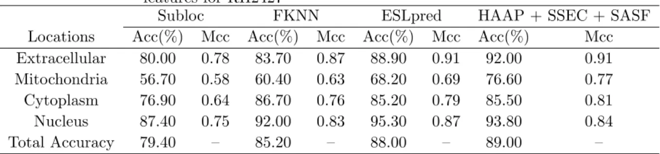
To validate the proposed method, we also compare it with other subcellular localisation prediction methods including SubLoc from Hua, FKNN from Huang and ESLpred from Bhasin. The comparison results are summarised in Table 2.2. The proposed method performs best among all methods. It outperforms fuzzy nearest neighbour using dipeptide feature almost 4% and binary SVM using AAC more than 9%. Our method is about 1% better than ESLpred in terms of total accuracy. However, for 3 out of 4 locations, our method works better than ESLpred in both accuracy and MCC values. Even though the overall accuracy is only 1% higher than ESLpred, it is already a big achievement on this data set. The main reason is that the data set contains 321 mitochondrial proteins (13% of entire data set). It is extremely hard to make improvement in prediction accuracy for mitochondria proteins, which prevent the further increase in total accuracy.
Table 2.2 Comparison with other best prediction methods using different features for RH2427
Subloc FKNN ESLpred HAAP + SSEC + SASF
Locations Acc(%) Mcc Acc(%) Mcc Acc(%) Mcc Acc(%) Mcc
Extracellular 80.00 0.78 83.70 0.87 88.90 0.91 92.00 0.91 Mitochondria 56.70 0.58 60.40 0.63 68.20 0.69 76.60 0.77
Cytoplasm 76.90 0.64 86.70 0.76 85.20 0.79 85.50 0.81
Nucleus 87.40 0.75 92.00 0.83 95.30 0.87 93.80 0.84
Total Accuracy 79.40 – 85.20 – 88.00 – 89.00 –
Table 2.3 Prediction accuracy comparison results for PK7579 data set
Location AAC (%) DPC(%) Park and Kanehisa (2003) (%) HAAP+SSEC(%)
Chloroplast 60.8 69.3 72.3 72.6 Cytoplasm 67.5 70.2 72.2 79.5 Cytoskeleton 55 62.5 58.5 65 ER 49.1 63.2 46.5 64.9 Extracellular 74.6 79.3 78 88.9 Golgi 12.8 27.7 14.6 55.3 Lysosome 66.7 63.4 61.8 81.7 Mitochondria 43.2 51.4 57.4 64.2 Nucleus 86.7 85.1 89.6 92.8 Peroxisome 16.8 28.8 25.2 34.4 Plasma 88.3 90.1 92.2 97.6 Vacuole 31.5 44.4 25 44.4 Total 73.1 76.2 78.2 84.4
We further applied our method to PK7579 data set, which contains 7579 proteins in 12 locations. The results are shown in Table 2.3. The predictions for using AAC, dipeptide and SSEC + HAAP features are all done using the multi-class SVM. Owing to computing resource limits and the fact that incorporating SASF results in less than a 1% improvement on accuracy (see Table 2.1), only the SSEC and HAAP features were implemented on this data set. For the same reason, we used five-fold cross-validation instead of leave-one-out. The grid search is also applied to find the best parameter values for SVM.
As shown in Table 2.3, the dipeptide feature works better than AAC since it incorporates the sequence order information. As expected, the combined feature of SSEC and HAAP performs better than dipeptide because it contains both structural and sequence information.
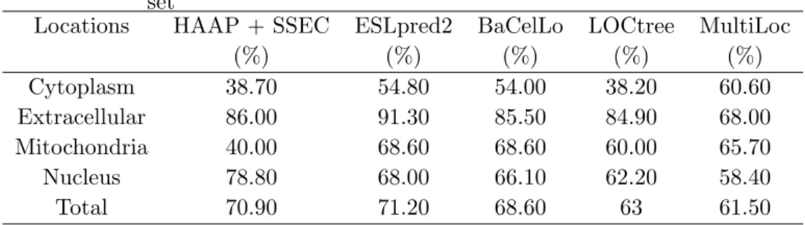
Table 2.4 The comparison of performance on the animal independent data set
Locations HAAP + SSEC ESLpred2 BaCelLo LOCtree MultiLoc
(%) (%) (%) (%) (%) Cytoplasm 38.70 54.80 54.00 38.20 60.60 Extracellular 86.00 91.30 85.50 84.90 68.00 Mitochondria 40.00 68.60 68.60 60.00 65.70 Nucleus 78.80 68.00 66.10 62.20 58.40 Total 70.90 71.20 68.60 63 61.50
The total accuracy 84.4% is achieved when using the combined feature. This is the best performance so far in the literature. Compared with Parks work, the total accuracy is improved about 6% using our method. The locations with fewer training samples, such as Golgi, ER and vacuolar, show the most improved accuracies. This provides a strong evidence for the usefulness of the proposed features. More importantly, we used only two features and it can be easily automated in future applications. However, Park used five different features and assembled 60 binary classifiers to improve the total accuracy to 78.2%.
Finally, we tested our method on the BaCelLo animal independent data set to compare the performance with the most recent best methods. To compare with other methods fairly, we retrained our classification model using HAAP and SSEC as features with 1890 training proteins and tested the performance on 707 testing proteins. The comparison of performance with other best available methods including BaCelLo, ESLpred2 (Garg and Raghava, 2008), MultiLoc (Hoglund et al., 2006) and LOCtree (Nair and Rost, 2005) is shown in Table 2.4. Our method can correctly predict 501 out of 707 proteins with a 70.9% total accuracy. It performs about 2%, 8%, 9% better on total accuracies compared with BaCelLo, LOCtree and MultiLoc, respectively, and about the same as ESLpred2. Specifically, our method can predict locations more accurately on nuclear and extracellular proteins with accuracies 78.8% and 86.0%, re-spectively. For locations with fewer training and testing proteins such as mitochondrion and extracellular, our method does not perform well since it focuses on the general performance for the whole data set.
Predicting locations in Arabidopsis
Arabidopsis is a well-known model organism and its protein sequences are available online at TAIR (Swarbreck et al., 2008). Unfortunately, most protein functions remain unknown and have not been characterised. We take the advantage of our high prediction accuracy method, and use PK7579 as the training data set to predict the subcellular locations for the entire Arabidopsis proteome. The HAAP and SSEC features are implemented in this application. The location with highest probability is assigned to each Arabidopsis protein. Figure 2.4 shows the percentage of each location in Arabidopsis proteome. A full list of Arabidopsis proteins and their predicted locations is available in the supplemental documentation for this paper.
Figure 2.4 The percentage of each location in Arabidopsis proteome
From the pie chart, we can see that nucleus proteins take about 40% in Arabidopsis pro-teome. This can be explained by the fact that most proteins are nucleus proteins from Stru-LocPred: Structure-based protein subcellular localisation prediction 11 our knowledge. On the other hand, membrane and cytoplasm proteins also have a high proportion partially because of the big amount of corresponding training proteins. Moreover, we checked the prediction results
with Arabidopsis Subcellular location database eSLDB (Pierleoni et al., 2007), which collects 2290 Arabidopsis proteins with experimentally determined locations. We took only those pro-teins annotated in eSLDB as Nucleus, Transmembrane, Cytoplasm, Extracellular and Plastid, and compare with their predicted locations to calculate the matching rate. 366 proteins are uniquely annotated as transmembrane proteins. More than 86% (316/366) of them match with our prediction results. A summary of the matching results for proteins with only one location listed in eSLDB is shown in Figure 2.5.
Figure 2.5 Percentage of proteins with known locations in eSLDB matches with predicted locations
StruLocPred server
The SVM modules and two protein features proposed in this paper have been imple-mented as web server StruLocPred using CGI python scripts. It is publicly available at http://wgzhou.ece.iastate.edu/StruLocPred/. The server allows the user to paste or type query protein sequence into the text area with FASTA format. It provides options for users to choose from SVM models trained with either RH2427 including 4 locations or PK7579 including 12 locations. Furthermore, the user is able to select any of the two proposed features, which are HAAP and SSEC, or their combination (Hybrid). The two conventional features AAC and
DPC are not implemented in the server since their performance is not satisfactory compared with our proposed features. The proposed feature SASF is not included as well because of re-source limit and the fact that it will not improve the performance greatly as stated in previous section. The prediction results consist of the predicted location and the corresponding prob-ability estimate using the chosen model. The predicted location is always the location with highest probability estimate across all locations. In the case of using SSEC as a feature, the output will include a fragment of the protein sequence and the predicted secondary structural element (H, E or C) for each residue. A sample output of prediction results is shown in Figure 2.6.
Figure 2.6 The sample output of prediction results from StruLocPred server
Conclusions and Discussions
Protein subcellular locations provide key clues for understanding the function of proteins. Computational prediction of subcellular localisation on the genome scale has become possible based only on amino acid sequences. In this paper, we proposed two structurebased features,
which are SSEC and solvent accessibility state frequency, and used a multi-class SVM to predict subcellular localisation. By testing on two benchmark data sets, we show that the prediction accuracies can reach 89.0% and 84.4%, respectively. These are comparable with the best accuracies in the literature even though we used fewer features with shorter vector length. We also compare the performance of our method with other best available methods based on an independent data set. The total accuracy of 70.9% is achieved. This shows that our method performs almost the best as ESLpred2.
We further applied this method to predict the subcellular locations for the entire Arabidop-sis proteome based on the secondary structural feature and HAAP. The percentage of each location in the proteome is illustrated. Most proteins are predicted to be nucleus proteins. This is feasible as most known proteins are from nucleus. From the matching results with 2290 known location proteins from eSLDB, 86% transmembrane protein locations match with their predicted ones. In general, the overall matching for proteins from five locations with the predicted locations is over 77%. This is very encouraging and demonstrates the effective-ness of the proposed structural features. Finally, the proposed SVM modules and features are implemented as web server at http://wgzhou.ece.iastate.edu/StruLocPred/.
Proteins have more opportunity to interact with proteins within the same subcellular lo-cation. Also, interacting proteins usually have similar functions. Interaction databases such as DIP (Salwinski et al., 2004) and BioGRID (Breitkreutz et al., 2008) are available now for several species. With the availability of proteome scale interaction network (Geisler-Lee et al., 2007), our next step will be to characterise proteins of unknown function by analysing their interacting partners from the same subcellular location in the interaction network. The subcellular location information can also provide additional evidence for verifying potential interactions.
3. MULTI-LABEL SUBCELLULAR LOCALIZATION PREDICTION BASED ON PROTEIN SEQUENCE AND STRUCTURAL FEATURES
A paper submitted to Journal of Bioinformatics and Computational Biology Wengang Zhou and Julie A. Dickerson
Abstract
Many proteins are located in multiple locations at different times and conditions. Cur-rent subcellular localization methods can only predict a single location for a given protein. We compare three multi-label classification methods based on binary and multi-class schemes using support vector machine, fuzzy k nearest neighbor, and extreme learning machine as clas-sifiers respectively. A new training and testing multi-label dataset is created from Uniprot for evaluating the performance of three proposed methods. Two protein features Hybrid Amino Acid Pair and Secondary Structural Element Composition help the multi-label prediction of subcellular locations. The results show that binary scheme outperforms multi-class scheme consistently for all three multi-label methods. The three methods achieve a similar microaver-age F-measure around 0.6 for binary scheme. The fastest and most stable multi-label method based on the support vector machine is implemented in a web server MLSubLoc. It is publicly available at http://wgzhou.ece.iastate.edu/MLSubLoc.
Introduction
Subcellular localization is a key functional characteristic of proteins. Proteins must be localized to correct cellular compartments to fulfill their biological roles. Experimental ap-proaches for determining subcellular locations are time-consuming and costly. Computational
methods can assign subcellular locations to proteins accurately, and gain functional clues for proteins from amino acid sequences. Numerous methods (Su et al., 2007; Lin et al., 2011) have been developed to predict single-label subcellular location using different classifiers and features.
Many proteins are present in multiple compartments to carry out different functions. Most proteins in Uniprot are experimentally annotated with multiple locations (Zhang et al., 2008). In mouse liver, 39% of all organellar proteins are in multiple locations (Foster et al., 2006). To the best of our knowledge, no research work has been conducted for multi-label prediction of subcellular locations. The multi-label subcellular localization prediction can provide a better picture for biologists to understand the function of proteins.
We develop three multi-label classification methods and evaluate them on a newly curated dataset using two previously described protein features. The best method is implemented in a web server named MLSubLoc. The server aims to help discover the actual function from the multiple predicted protein subcellular locations.
Protein Features
We proposed two novel protein features named Hybrid Amino Acid Pair (HAAP) and Secondary Structural Element Composition (SSEC) in previous work (Zhou et al., 2011). These features were shown to perform better than traditional features for single-label subcellular location prediction problems.
The HAAP is a sequence based feature. It is a combination of dipeptide and amino acid pairs with a gap (Park et al., 2003). There are total 400 types of amino acid pairs (AAPs). For each pair, we calculate its total number of occurrence between any two residues adjacently and with a gap. The fraction can be computed by the following equation:
F raction of dipeptide(i) = T otal number of dipeptide i
T otal number of dipeptides in the sequence (3.1)
The SSEC represents frequencies of secondary structural elements (H, E, C) for each residue in a given protein sequence. H, E and C represent alpha helix, beta sheet and other structures
respectively. The frequencies are calculated according to the following formula:
fik= N
k i
L (3.2)
Where i = (H, E, C); fik is the frequency of secondary structural element i occurring at
amino acid k and Nik is the total number of structural elements i found for amino acid k in
the whole protein sequence. Lis the length of the protein sequence. The secondary structure prediction is made by PSIPRED 2.5 (Jones, 1999).
Classifiers Review Support Vector Machine
The SVM (Vapnik, 1995) is a statistical learning method first proposed by Vapnik. It is based on the theories of VC dimension and structure risk minimisation. For two-class classification problems, SVMs use a non-linear mapping known as a kernel function to map the training data into a higher dimensional feature space, and then construct an optimal separating hyperplane in the higher dimensional space corresponding to a non-linear classifier in the input space. With the kernel functions and the high dimensional space, the hyperplane computation requires solving a quadratic programming problem:
minw,b,ξ 1 2kwk 2 +CX i ξi (3.3) s.t.:yi(w·xi+b)≥1−ξi, i= 1,· · ·, m (3.4) C is a tuning parameter that allows the user to control the trade-off between classifying the training samples without error and maximising the margin.
The three commonly used kernel functions include linear kernel, polynomial kernel and Radial Basis Function (RBF) kernel. The RBF kernel with a parameter γ (gamma) is shown in the following equation:
We used the SVM classifier implemented in LIBSVM 2.85 (Chang et al., 2001). RBF kernel is used in all our simulations. The penalty parameter C and RBF kernel parameter are tuned for each dataset using grid search program from LIBSVM to get the best performance.
Fuzzy K-Nearest Neighbor
K nearest neighbor (KNN) systems classify a testing sample according to its k nearest neighbors in the training samples with known classification labels. The sample is then assigned to the class that has the maximum number of neighbors.
Fuzzy k nearest neighbor (FKNN) (Keller et al., 1985; Sim et al., 2005) extends the KNN by introducing a fuzzy membership function and a distance weight. Fuzzy membership can be used to estimate the confidence level to each class and the weight raises the distance to k nearest neighbors to a certain power for the testing sample. The membership value ui(x) to
class i is calculated by the following formula:
ui(x) = Pk j=1ui(x(j))( x−x (j) −2/(m−1) ) Pk j=1( x−x(j) −2/(m−1) ) i= 1, ..., c (3.6)
Where k is the number of neighbors used and m is the fuzzifier variable which determines how the membership varies with distance.
Extreme Learning Machine
Extreme learning machines (ELM) were first proposed by Huang et al. in 2004. It is a new fast learning algorithm for single hidden layer feed forward neural network. The neural network structure is shown in Figure 3.1. It consists of three layers: input, hidden and output. The edges between input and hidden layers are called input weights. Similarly, edges linking the hidden layer and output layer are named output weights. Normally, the input weights are generated randomly at first. Both input and output weights will be adjusted during the training stage.
Given N distinct samples (Xj, Yj), where Xj is the n-dimensional feature vector of jth
Figure 3.1 Extreme Learning Machine Network Structure
network (SLFN) withM hidden neurons and activation function f(x) can be mathematically modeled as:
M X
i=1
Oif(Wi·Xj+Bi) =Tj, j= 1,2, ..., N (3.7)
Where Wi is the input weight vector between ith hidden neuron and all input neurons,
Oi = (Oi1, Oi2, , Oim) is the output weight vector connecting hidden layer and output layer
and m is the number of output neurons, Bi is the hidden biases vector with M dimension.
There exists a SLFN withO, B, andW that can approximate those given samples with zero errorPN
j=1kTj−Yjk= 0. Therefore, the previous equation can also be written in the matrix
format as: HO =Y. WhereY = (Y1, Y2, , YN)N×m,H =f(Wi·Xj+Bi)N×M andOM×m can
be calculated by Moore-Penrose Generalized Inverse.
Multi-label Classification
Multi-label classification associates each sample with a set of labels. We implemented three multi-label classification methods based on binary and multi-class approaches using Support Vector Machine, Extreme Learning Machine, and Fuzzy K Nearest Neighbor as classifiers. These three methods are referred as MLSVM, MLELM, and MLFKNN respectively.
For the binary approach, a binary classifier is built for each label (subcellular location). The samples associated with that label are assigned to one class and the rest are in another class. The final labels for the testing sample are the combination of predicted labels from all binary classifiers. The binary multi-label classification scheme is illustrated in Figure 3.2 in detail.
Figure 3.2 Binary multi-label classification scheme
For multi-class approach, the original label sets are organized into a few classes. The same label sets are put into one class. We then simply solve a multi-class classification problem. The multi-class SVM based on one versus one strategy implemented in Libsvm is used in this work. FKNN and ELM are multi-class classifiers inherently.
The binary datasets are highly unbalanced as there are only a small proportion of positive samples. Therefore, balanced accuracy (Yang et al., 2008) is used as the evaluation criterion to find the best parameters for each classifier. The best SVM parameters are found using grid search method in LIBSVM for each binary classifier Ch. Balanced accuracy (BAC) is defined
Balanced Accuracy= Sensitivity+Specif icity 2 (3.8) Sensitivity(Recall) = T P T P +F N (3.9) Specif icity= T N T N+F P (3.10)
Where T P,F N,T N, andF P represent true positives, false negatives, true negatives and false positives respectively.
Experiment Results Dataset
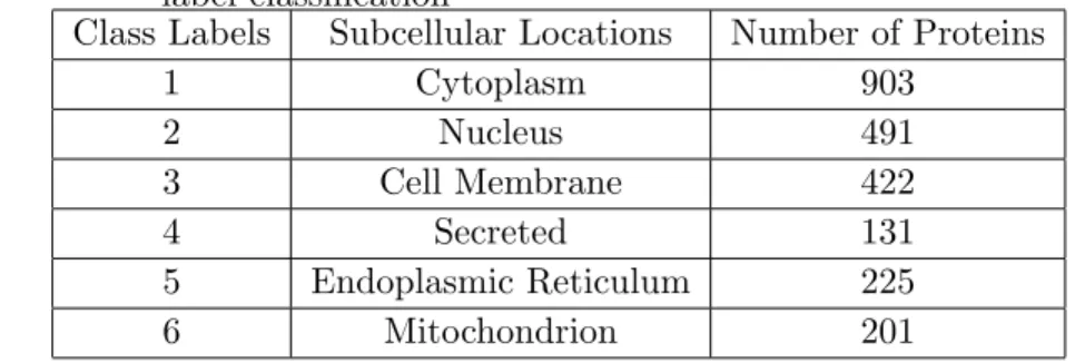
All protein sequences are collected from Uniprot/Swissprot database (The UniProt Con-sortium, 2010) release 2010 09. We used eukaryotic proteins with available subcellular location annotation information in the CC (comments) field. Proteins annotated with potential, prob-ably and by similarity are not included. We only keep proteins with at least two annotated locations from the following six subcellular locations: 1. Cytoplasm, 2. Nucleus, 3. Cell Membrane, 4. Secreted, 5. Endoplasmic Reticulum, and 6. Mitochondrion.
Furthermore, any protein sequences with less than 50 amino acids or with irregular charac-ters such as Z, X, and B are excluded from the dataset. Sequences with a high degree similarity are also removed by all-to-all sequence similarity search using the program BLASTCLUST. Proteins with more than 30% similarity in the full length are grouped into different clusters. Any two proteins in the same cluster are deemed to be too similar for use by prediction meth-ods. Therefore, we randomly pick one protein from each cluster. After these cleaning steps, 1118 remaining proteins located in at least two out of the six locations are summarized in Table 3.1.
Table 3.1 The number of proteins in each location used for binary multi--label classification
Class Labels Subcellular Locations Number of Proteins
1 Cytoplasm 903 2 Nucleus 491 3 Cell Membrane 422 4 Secreted 131 5 Endoplasmic Reticulum 225 6 Mitochondrion 201
Table 3.2 The best parameters found and the corresponding balanced ac-curacy (BAC) values for each label in MLSVM using HAAP and SSEC features
Class Labels SSEC HAAP
C γ BAC C γ BAC 1 4096 2 0.57 1024 2 0.59 2 4 128 0.62 64 2 0.59 3 4 128 0.64 4 512 0.6 4 16384 0.5 0.65 16 128 0.62 5 64 8 0.55 16384 0.125 0.58 6 4096 8 0.59 256 32 0.58 Parameter Setting
The original training and testing datasets contains 894 (80% total) and 224 (20% total) proteins respectively. For each label (subcellular location) in the training dataset, a binary classifier will be built and trained. The parameters that achieve the best 5-flod cross validation performance for that classifier are kept for later use in the testing stage.
The grid search method in LIBSVM is used to find the best parameter value combination ofC andγ for binary scheme MLSVM from the range of [2−10,2−9,· · ·,210] with step size 22. The parameter values of C and γ used in MLSVM and their corresponding BAC values for each label are listed in Table 3.2.
The two parameters in FKNN classifier are set as k= 15 andm = 1.2 in all experiments in this work. For ELM, we use sigmoid function f(x) = 1+1e−x as the activation function
experimental observation.
Evaluation Measurements
For assessing the performance of different multi-label methods, we defined two evaluation measurements: Exact Match Ratio (EMR) and Microaverage F-measure (MF). EMR and MF are calculated according to the following formulas:
EM R= N umber of correctly predicted samples
T otal number of testing samples (3.11)
M F = 2·P recision·Recall
P recision+Recall (3.12)
P recision= T P
T P +F P (3.13)
Where T P and F P refer to true positives and false positives respectively. Recall is the same as sensitivity defined in the previous section.
EMR requires all predicted labels have to match with all target labels for a testing sample. In most cases, it is very hard to achieve a complete match between two label sets. There-fore, EMR is expected to be comparatively low. MF is a comprehensive measurement as it takes partial matches between predicted and target labels into account by incorporating both precision and recall.
Performance Comparison
We compare the performance of three multi-label classification methods using both binary and multi-class approaches.
Binary Multi-label Scheme
The performance of three multi-label methods using binary approach is evaluated using protein features SSEC, HAAP, and their combination SSEC+HAAP on the original dataset
Table 3.3 The comparison of different binary multi-label methods using SSEC, HAAP, or their combination as features
Multi-label SSEC HAAP SSEC+HAAP
Methods EMR MF EMR MF EMR MF
MLSVM 0.18 0.62 0.16 0.59 0.20 0.63
MLFKNN 0.22 0.61 0.23 0.60 0.22 0.62
MLELM 0.16 0.59 0.15 0.59 0.14 0.61
Table 3.4 CPU time (in seconds) used on the testing dataset for all three methods
Methods SSEC HAAP SSEC+HAAP
MLSVM 5.7 13.9 19.3
MLFKNN 30.1 98.7 132.3
MLELM 27.3 87.5 116.0
as listed in Table 1. The comparison results of the three methods MLSVM, MLFKNN and MLELM are shown in detail in Table 3.3.
As observed from the table, MLSVM and MLELM have similar performance using either SSEC or HAAP as features. MLFKNN performs a little better with respect to EMR measure-ment than the other two methods. In general, MF values obtained from all three methods are around 0.6. The combined feature does improve the prediction ability slightly.
In addition to evaluate the proposed methods based on EMR and MF, we also investigated the running time cost of each method. The CPU time consumed by three multi-label methods using two different features is summarized in Table 3.4. Although the comparable performance of the three methods in terms of microaverage F-measure, their running time has a big differ-ence. MLSVM runs about 6 to 7 folds faster than MLFKNN and MLELM methods using all three features. The running time using the combined feature is much longer than using the other two features. All three multi-label methods run fastest when the SSEC feature is used.
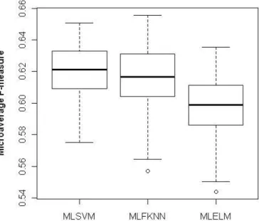
To test the stability of three proposed methods, we run each method 100 times. Each time a new dataset is created from the original dataset by random sampling without replacement. The first 80% proteins are chosen as training with all the rest as testing samples. The MF values in 100 runs are recorded for each method. The two box plots showing MF changes using
SSEC and HAAP features are shown in Figures 3.3 and Figure 3.4.
Figure 3.3 The box plot of MF values in 100 runs using SSEC feature
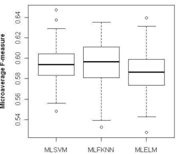
From both figures, we observe that MLSVM is always the most stable method with very small variance on MF values using both features. MF medians obtained from MLSVM and MLFKNN are almost the same. In both cases, MLELM has the worst performance. For using SSEC feature, MLSVM perform better than the other two methods.
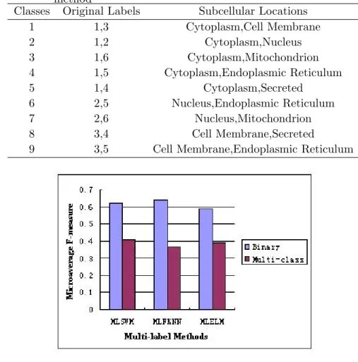
Multi-class Multi-label Scheme
To perform the multi-label classification with multi-class approach, we create a new dataset with 933 proteins extracted from the original 1118 proteins. The new dataset is organized into 9 classes. The detailed class information is specified in Table 3.5.
We select 80% of the 933 proteins for training and the remaining 20% as testing, and test the performance of the three multi-label methods MLSVM, MLFKNN, and MLELM in multi-class scheme using both SSEC and HAAP features.
The bar plots comparing MF values obtained from binary and multi-class approaches using SSEC and HAAP features are shown in Figures 3.5 and 3.6 respectively. The MF values for
Figure 3.4 The box plot of MF values in 100 runs using HAAP feature
binary approach are taken from Table 3.3.
As seen from the figures, for the multi-class scheme, MLSVM performs slightly better than the other two methods as well and achieves a microaverage F-measure around 0.4 using both features. All three methods achieve higher MF values using SSEC compared to HAAP.
We also observe that binary approach consistently outperforms multi-class approach for all three multi-label methods in terms of Microaverage measure using both features. The F-measures for multi-class methods are about 20% lower than their corresponding binary methods using the same classifier.
MLSubLoc Server
Due to the good performance and the fast running speed, we implement the method MLSVM and two protein features in a web server named MLSubLoc for the prediction of mul-tiple subcellular locations. The server is developed using PHP and Python scripts. MLSubLoc server and supplementary data are publicly accessible at: http://wgzhou.ece.iastate.edu/MLSubLoc.
Table 3.5 933 proteins used for multi-class multi-label classificaiton method
Classes Original Labels Subcellular Locations
1 1,3 Cytoplasm,Cell Membrane 2 1,2 Cytoplasm,Nucleus 3 1,6 Cytoplasm,Mitochondrion 4 1,5 Cytoplasm,Endoplasmic Reticulum 5 1,4 Cytoplasm,Secreted 6 2,5 Nucleus,Endoplasmic Reticulum 7 2,6 Nucleus,Mitochondrion 8 3,4 Cell Membrane,Secreted
9 3,5 Cell Membrane,Endoplasmic Reticulum
Figure 3.5 The comparison between binary and multi-class approaches for three multi-label methods using SSEC feature
either of the two implemented multi-label classification approaches, binary and multi-class. It also provides options for user to select from a combination of three protein features, SSEC, HAAP, and SSEC+HAAP. The web interface screenshot is shown in Figure 3.7.
The output differs depending on the different chosen multi-label approaches and protein features. For the binary approach, MLSubLoc only displays the predicted multiple subcellular locations. For the multi-class scheme, the probability estimates for predicted locations are displayed. When using SSEC as the feature, the output will also include a fragment of the protein sequence and the predicted secondary structural element (H, E or C) for each residue.
Figure 3.6 The comparison between binary and multi-class schemes for three multi-label methods using HAAP feature
Figure 3.8 shows a sample output of the prediction results.
Conclusions
Three multi-label classification methods are implemented for predicting multiple subcellular locations for a give protein. The performance of three multi-label methods MLSVM, MLFKNN, and MLELM are compared between binary and multi-class schemes using different protein features. The results show that binary scheme performs better than multi-class scheme for all three methods using both SSEC and HAAP features. MLSVM is the most stable method and has the shortest running time. The method MLSVM in binary and multi-class schemes and three protein features are implemented in a web server named MLSubLoc. The server is publicly accessible at http://wgzhou.ece.iastate.edu/MLSubLoc. The ability of predicting multiple locations will facilitate other analysis such as protein-protein interaction network modeling (Geisler-Lee et al., 2007).
Figure 3.7 MLSubLoc server takes a protein sequence as input and allows users to choose any of the three features
Figure 3.8 The sample output of MLSubLoc server using SSEC feature and binary multi-label classification approach
4. A NOVEL CLASS DEPENDENT FEATURE SELECTION METHOD FOR CANCER BIOMARKER DISCOVERY
A paper submitted to IEEE/ACM Transactions on Computational Biology and Bioinformatics
Wengang Zhou and Julie A. Dickerson
Abstract
Identifying key biomarkers for different cancer types can improve diagnosis accuracy and treatment. Gene expression data can help differentiate between cancer subtypes. However the limitation of having a small number of samples versus a larger number of genes represented in a dataset leads to the overfitting of classification models. Feature selection methods can help select the most distinguishing feature sets for classifying different cancers. A new class depen-dent feature selection approach integrates the F statistic, Maximum Relevance Binary Particle Swarm Optimization (MRBPSO) and Class Dependent Multi-category Classification (CDMC) system. This feature selection method combines filter and wrapper based methods. A set of highly differentially expressed genes (features) are pre-selected using the F statistic for each dataset as a filter for selecting the most meaningful features. MRBPSO and CDMC function as a wrapper to select desirable feature subsets for each class and classify the samples using those chosen class-dependent feature subsets. The performance of the proposed methods is evaluated on eight real cancer datasets. The results indicate that the class-dependent approaches can effectively identify biomarkers related to each cancer type and improve classification accuracy compared to class independent feature selection methods.