OpenCommons@UConn
Doctoral Dissertations
University of Connecticut Graduate School
5-25-2017
Bayesian Modeling and Inference for Nonignorably
Missing Longitudinal Response Data
Jing Wu
Follow this and additional works at:
https://opencommons.uconn.edu/dissertations
Recommended Citation
Wu, Jing, "Bayesian Modeling and Inference for Nonignorably Missing Longitudinal Response Data" (2017).Doctoral Dissertations. 1411.
Nonignorably Missing Longitudinal Response Data
Jing Wu, Ph.D.
University of Connecticut, 2017
Missing data are frequently encountered in longitudinal clinical trials. To better moni-tor and understand the progress over time, we must handle the missing data appropriately and thus examine whether the missing data mechanism is ignorable or nonignorable.
In this dissertation research, we develop models and carry out Bayesian inferences for both longitudinal binary response and count response data. For longitudinal binary re-sponse data, we develop a new probit model. It resolves the well-known weak identifiability issue of the variance of the random effects, and substantially improves the convergence and mixing of the Gibbs sampling algorithm. We adopt a sequence of one-dimensional condi-tional distributions for the missing data indicators via a logistic regression model. For the longitudinal count response data, we use the zero-inflated Poisson model for the response measurements, and propose a new conditional model for the missing data mechanism. The new model has the potential of reducing the number of nuisance parameters, allows us to model dropout and intermittent missing jointly, and provides a broad class of missing data mechanisms. We then investigate and characterize the conditions for propriety of the joint posterior distribution under both binary and Poisson cases, and propose a variation of Jeffreys’s prior as a remedy for impropriety of the posterior. In addition, we develop two efficient Gibbs sampling algorithms for both binary and Poisson cases, which allow us
to conveniently sample missing responses and to apply the collapsed Gibbs technique as well as the hierarchical centering technique within the Gibbs sampling framework.
The proposed methodologies and the sampling techniques are illustrated using real data from an HIV prevention clinical trial. A sensitivity analysis is carried out to assess the robustness of the posterior estimates under different prior specifications and missing data mechanisms. Two model assessment criteria, the deviance information criterion (DIC) and the logarithm of the pseudomarginal likelihood (LPML), are used to examine model fit. Extensive real data analyses are conducted to assess the performances of missing data mechanisms under different scenarios.
Nonignorably Missing Longitudinal Response Data
Jing Wu
B.S., Shanghai Jiao Tong University, China, 2012
A Dissertation
Submitted in Partial Fulfillment of the Requirements for the Degree of
Doctor of Philosophy at the
University of Connecticut 2017
Jing Wu
2017
Doctor of Philosophy Dissertation
Bayesian Modeling and Inference for
Nonignorably Missing Longitudinal Response Data
Presented by Jing Wu, B.S. Major Advisor Ming-Hui Chen Major Advisor Elizabeth D. Schifano Associate Advisor Jun Yan University of Connecticut 2017 iii
First and foremost, I would like to express my deep gratitude to my major advisor Prof. Ming-Hui Chen for his continuous support through all these years. Prof. Chen has sup-ported me not only by providing the unique assistantship and collaboration opportunities, but also being an incredibly wonderful academic and life mentor. I would like to thank him for leading me to the research area of statistics, partnering with me on the accumulation of advanced statistical knowledge, and inspiring me to pursue teaching and research as my lifetime career. Choosing him as my advisor is one of the best decisions I have made. I gratefully acknowledge my co-major advisor Prof. Elizabeth D. Schifano for her great guidance and insightful advice, which are extremely important to me in the whole process of my graduate study.
I would like to thank my associate advisor Prof. Jun Yan for all the kind help and advice on my job application and research work.
Special thanks to Pfizer Inc. for offering me the research fellow position and provid-ing me the precious two-year industry experience. I would like to especially thank Dr. Huaming Tan and Dr. Neal Thomas for imparting me the pharmaceutical knowledge, and giving me advice on both professional and personal development.
My sincere thanks also goes to the Center for Nursing Research for supporting my half-time graduate assistantship during the past three academic years. I am particularly thankful to Ms. Elise Bennett, Prof. Xiaomei Cong, Prof. Stephen Walsh, and Wanli Xu for their warmth and support.
It is my great honor to work with and learn from Dr. Anthony V. D’Amico of Harvard Medical School. This invaluable opportunity substantially enhances my understanding of survival analysis.
and company that makes my journey to the Ph.D. more delightful. I would also like to thank Ms. Tracy Burke and Ms. Megan Petsa for their helpful administrative assistance. Lastly, and most importantly, I want to dedicate this dissertation to my mother Yalian Chen and my father Guohui Wu, who always encourage and support me to pursue the life and career I adore. It is your unconditional love that leads me to conquer and to achieve.
Chapter 1: Introduction 1
1.1 Literature Review . . . 1
1.2 HIV Prevention Behavioral Intervention Clinical Trials . . . 3
1.3 Motivating Data . . . 5
1.4 Methodologies Overview . . . 9
1.5 Dissertation Outline . . . 11
Chapter 2: Models for Longitudinal Binary Response Data 12 2.1 The Proposed Models . . . 12
2.1.1 The Model for Longitudinal Binary Measurements . . . 12
2.1.2 Missing Data Mechanism . . . 15
2.2 Bayesian Inference . . . 16
2.2.1 The Likelihood Function . . . 16
2.2.2 Prior and Posterior Distributions . . . 17
2.2.3 Computational Development . . . 20
2.2.4 Bayesian Model Assessment . . . 25
2.3 A Simulation Study . . . 27
2.4 Analysis of the HIV Prevention Behavioral Data . . . 32
Chapter 3: Models for Longitudinal Count Response Data 42 3.1 The Proposed Methods . . . 42
3.1.1 The Model for Longitudinal Counts . . . 42
for Intermittent Missing . . . 44
3.1.3 Predictive Probabilities of Dropout and Intermittent Missing . . . . 48
3.2 Bayesian Inference . . . 49
3.2.1 The Likelihood Function . . . 49
3.2.2 Adjusted Intervention Effect . . . 50
3.2.3 Prior and Posterior Distributions . . . 51
3.2.4 Computational Development . . . 53
3.2.5 Bayesian Model Assessment . . . 60
3.3 Analysis of the HIV Prevention Behavioral Data . . . 62
Chapter 4: Assessment of Missing Data Mechanism 73 4.1 Motivation . . . 73
4.2 Assessment of Missing Data Mechanism in Section 2.1.2 . . . 74
4.3 Assessment of Missing Data Mechanism in Section 3.1.2 . . . 77
Chapter 5: Extension and Future Research Direction 87 5.1 Extensions to Choice of Link Functions . . . 87
5.2 Extensions to Missing Data Mechanism and Multiple Longitudinal Outcomes 88 5.2.1 Path Specific Model . . . 88
5.2.2 Joint Modeling of Multiple Types of Responses. . . 90
5.3 Extensions to Model Selection Criteria . . . 91
Appendix A: Proofs of Theorems 92
Appendix B: Additional Tables 97
1.1 Characteristics of Study Participants (N=1875) . . . 6
1.2 Missing Pattern of the Count Responses (ACASI-reported number of un-protected sex acts).. . . 8
2.1 Posterior Summaries under the Nonignorable Model with a N(0, 6) Prior and Jeffreys Prior When the Missingness Percentages Were 5.37%, 10.52%, 11.94%, and 14.18% . . . 33
2.2 Posterior Summaries under the Nonignorable Model with a N(0, 8) Prior and Jeffreys Prior When the Missingness Percentages Were 5.37%, 10.52%, 11.94%, and 47.14% . . . 34
2.3 Values of DICR|y(pD) and LPMLR|yunder Ignorable Missingness and
Non-ignorable Missingness with Various Priors for the HIV Prevention Behav-ioral Data . . . 35
2.4 Posterior Summaries under the Ignorable Model for the HIV Prevention Behavioral Data . . . 39
2.5 Posterior Summaries under the Nonignorable Model with a N(0,8) Prior
for the HIV Prevention Behavioral Data . . . 40
2.6 Posterior Summaries under the Nonignorable Model with Jeffreys Prior for the HIV Prevention Behavioral Data . . . 41
3.1 Values of DICW,R|y(pD) and LPMLW,R|y under Ignorable Missingness and
Nonignorable Missingness with Various Priors for the HIV Prevention Be-havioral Data . . . 63
Data. . . 68
3.3 Posterior Summaries under the Nonignorable Model with aN(0,9) Prior for the HIV Prevention Behavioral Data. . . 69
3.4 Posterior Summaries under the Nonignorable Model with Jeffreys Prior for the HIV Prevention Behavioral Data. . . 70
3.5 Posterior Summaries of the Adjusted Overall Intervention Effect under the Ignorable Model, Nonignorable Model with a N(0, 9) Prior and Jeffreys Prior. 72 4.1 Values of DICR|y (pD) and LPMLR|yfor Longitudinal Binary Variable and
Longitudinal Poisson Variable under Ignorable Missingness and Nonignor-able Missingness with Various Priors for the HIV Prevention Behavioral Data . . . 75
4.2 Posterior Summaries of the Adjusted Overall Intervention Effect under the Ignorable Model, Nonignorable Model with a N(0, 7) Prior and Jeffreys Prior. 77 4.3 Posterior Summaries under the Ignorable Model for the HIV Prevention
Behavioral Data. . . 78
4.4 Posterior Summaries under the Nonignorable Model with a N(0,7) Prior
for the HIV Prevention Behavioral Data. . . 79
4.5 Posterior Summaries under the Nonignorable Model with Jeffreys Prior for the HIV Prevention Behavioral Data. . . 80
4.6 Values of DICW,R|y(pD) and LPMLW,R|yfor Longitudinal Binary Variable
and Longitudinal Poisson Variable under Ignorable Missingness and Nonig-norable Missingness with Various Priors for the HIV Prevention Behavioral Data . . . 81
Data. . . 83
4.8 Posterior Summaries under the Nonignorable Model with aN(0,8) Prior for the HIV Prevention Behavioral Data. . . 84
4.9 Posterior Summaries under the Nonignorable Model with Jeffreys Prior for the HIV Prevention Behavioral Data. . . 85
B.1 Posterior Summaries under the Nonignorable Model with a N(0, 1) Prior and a N(0, 10) Prior when missing percentage is low. . . 97
B.2 Posterior Summaries under the Nonignorable Model with a N(0, 1) Prior and a N(0, 10) Prior when missing percentage is high. . . 98
1.1 Path Diagram of the binary responses (any unprotected sex acts), where 0 in circle indicates observed and 1 in circle indicates missing; and the two numbers in parentheses indicate the number of zero counts (the first, blue) and the number of ones (the second, red) of the binary response variable at each visit on the specific path. . . 7
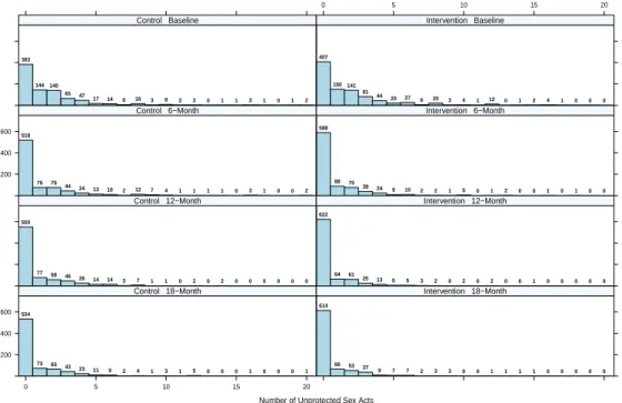
1.2 Trellis plots of the count responses (ACASI-reported number of unprotected sex acts). . . 9
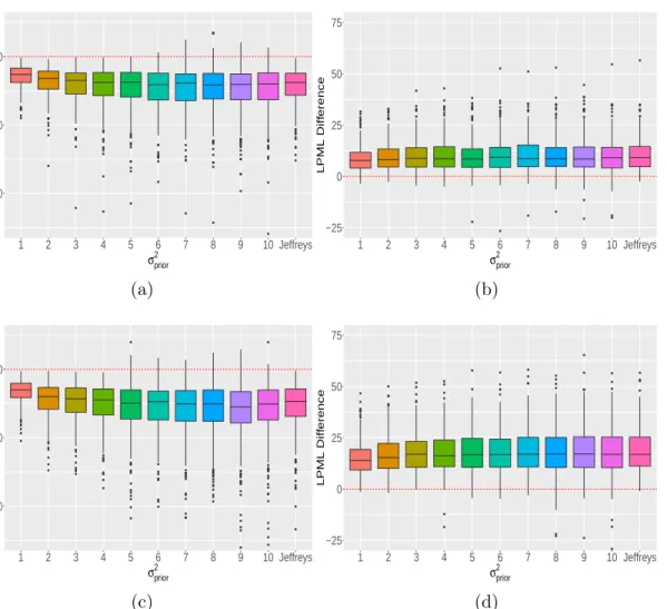
2.1 Plots of the DIC differences (a) and the LPML differences (b) when the missingness percentages were 5.37%, 10.52%, 11.94%, and 14.18%; and plots of the DIC differences (c) and the LPML differences (d) when the missingness percentages were 5.37%, 10.52%, 11.94%, and 47.14%. . . 30
Introduction
1.1 Literature Review
Intermittent missingness and dropout are frequently encountered in longitudinal stud-ies. Intermittent missingness occurs when the subject returns to the study after missing one or more visits and dropout refers to the situation where the subject permanently withdraws from the study.
Little and Rubin (2002) classified the type of missingness into three categories, “Miss-ing Completely at Random ” (MCAR) is where the probability of miss“Miss-ingness does not depend on either the observed or unobserved data. “Missing at Random” (MAR) is the situation where the probability of missingness does not depend on the unobserved data conditional on the observed data. “Missing Not at Random” (MNAR) is the setting in which the probability of missingness depends on the unobserved data. MCAR and MAR are typically referred to as ignorable missing data mechanisms since the missing data mech-anism does not need to be included in the likelihood specification, while MNAR is referred to as a nonignorable missing mechanism for obtaining the maximum likelihood estimates.
Nonignorable missing data is most frequently encountered in longitudinal studies, where data is gathered for the same subject repeatedly over time.
One approach for handling missing data is listwise deletion, in which all cases with missing values are deleted. This approach, however, introduces bias if the missingness is not MCAR. For MAR, inferential methods include maximum likelihood (Rubin, 1976; Ibrahim et al., 1999; Newman, 2003; Ibrahim et al., 2005), multiple imputation (Rubin, 2004; Royston and others, 2004; Sterne et al., 2009) and weighted estimating equations (Robins and Rotnitzky, 1995; Preisseret al., 2002). If the data are MNAR, one approach is to specify a parametric model for the missing data mechanism, and then jointly model the response variables and the missing data mechanism by incorporating them into the complete data log-likelihood. Three commonly used joint models are selection (Glynn
et al., 1986), pattern-mixture (Little, 1993), and shared-parameter models (Follmann and
Wu, 1995).
Ibrahimet al.(2001) proposed a general joint multinomial model for the missing data mechanism for longitudinal data, which nicely accommodates nonignorable missing re-sponse data with nonmonotone missingness patterns. They also devised a Monte Carlo EM algorithm, and derived the analytical form of the E- and M-steps for the normal random effects model. Huang et al. (2005) provided theoretical justifications of model identifiability for generalized linear models with nonignorably missing covariates where they mainly focused on missing covariates rather than missing response measurements. Albert (2000) considered the transition model, which is appropriate if one is interested in how the response and covariates are related to the missingness path of each subject. He examined the setting of intermittent missingness and proposed a transition model for lon-gitudinal binary data which allows for nonignorable intermittent missingness and dropout
of each subject. However, the model does not allow for correlations between the response variable within each subject, and it also does not consider the fact that an intermittent missing value at timetmust be followed by an observed value at some time point greater
than t(otherwise, it would be a dropout).
1.2 HIV Prevention Behavioral Intervention Clinical Trials
HIV, the human immunodeficiency virus, is a virus that attacks cells of the immune system (CD4) and interferes with the body’s ability to fight infections. If left untreated, HIV will ultimately lead to acquired immunodeficiency syndrome (AIDS). According to the statistics from AIDS.GOV, 36.7 (0.5%) million people worldwide are currently suffering from HIV/AIDS. So far, there is no treatment that can eradicate the HIV virus. The most effective therapy against HIV is called antiretroviral therapy (ART), which is the combination of several antiretroviral medicines used to suppress the progression of HIV disease.
In addition to the medical treatment, HIV prevention behavioral intervention also plays a critical role in reducing the unprotected sexual risk behavior, and prevent the growth of the virus. As has been widely recognized, HIV treatment as prevention should be bundled with behavioral interventions to maximize effectiveness (Kalichman et al., 2011).
More and more emphasis has been placed on HIV prevention behavioral research. Koblinet al.(2012) tested the efficacy of an HIV prevention behavioral intervention to re-duce sexual risk among African-American men who have sex with men (MSM). Kalichman
et al.(2011) concluded that a theory-based integrated behavioral intervention can improve
HIV treatment adherence and reduce HIV transmission risks. Moreover, there is a need for combination prevention as there is for combination treatment. Combination prevention should be based on scientifically derived evidence, with input and engagement from local communities that fosters the successful integration of care and treatment (Bekker et al., 2012).
In this dissertation research, we consider the data from an HIV prevention behavioral intervention clinical trial (Fisheret al., 2014) in South Africa from June 2008 to May 2010, where people living with HIV (PLWH) on antiretroviral therapy (ART) constitute a large population. However, a significant proportion of them do not achieve viral suppression. They serve as relatively healthy but infectious vectors for transmission of HIV virus. PLWH who engage in unprotected sex also place themselves at risk for other sexually transmitted infections, associated morbidity, and accelerated progression of HIV disease.
To reduce the risk, an one-on-one counseling session with trained lay counselors concerning sexual risk behavior reduction is introduced. The goal of this trial was to understand if a brief counseling intervention can significantly reduce HIV risk behavior among HIV-infected South Africans on ART.
1.3 Motivating Data
The data from the HIV prevention behavioral intervention clinical trial we consider were collected from sixteen urban, peri-urban, and rural primary healthcare clinics and community health centers in the uMgungundlovu and uMkhanyakude health districts of KwaZulu-Natal, South Africa from June 2008 to May 2010. The sixteen health districts were then randomized to intervention (8 clinics) and standard of care (8 clinics) arms. The total number of HIV-infected participants on ART was 1891 (967 for intervention and 924 for standard of care).
PLWH were invited to take part in the study and provided informed consent. Par-ticipation consisted of (1) completing audio computer- assisted self-interviews (ACASI) and interviewer-administered questionnaires at baseline, 6, 12, and 18 months, (2) pro-viding biological samples assessing sexually transmitted infections (STIs) at baseline, 12, and 18 months, and (3) consenting to medical chart reviews for CD4 count, HIV viral load, STIs, and health status. As part of routine clinical care, participants in the in-tervention (n = 967) and standard of care (n = 924) arms received counseling from lay counselors concerning issues relevant to PLWH on ART (e.g., adherence education and counseling). Participants at the 8 intervention clinics (n = 967) received brief, theory and evidence-based, tailored, one-on-one counseling sessions with trained lay counselors con-cerning sexual risk behavior reduction. Standard of care participants received standard of
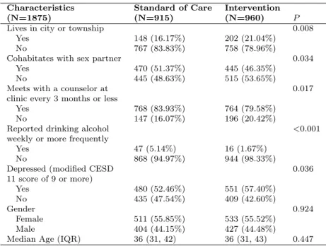
Table 1.1: Characteristics of Study Participants (N=1875)
Characteristics Standard of Care Intervention
(N=1875) (N=915) (N=960) P
Lives in city or township 0.008
Yes 148 (16.17%) 202 (21.04%)
No 767 (83.83%) 758 (78.96%)
Cohabitates with sex partner 0.034
Yes 470 (51.37%) 445 (46.35%)
No 445 (48.63%) 515 (53.65%)
Meets with a counselor at 0.017
clinic every 3 months or less
Yes 768 (83.93%) 764 (79.58%)
No 147 (16.07%) 196 (20.42%)
Reported drinking alcohol <0.001
weekly or more frequently
Yes 47 (5.14%) 16 (1.67%)
No 868 (94.97%) 944 (98.33%)
Depressed (modified CESD 0.036
11 score of 9 or more) Yes 480 (52.46%) 551 (57.40%) No 435 (47.54%) 409 (42.60%) Gender 0.924 Female 511 (55.85%) 533 (55.52%) Male 404 (44.15%) 427 (44.48%)
Median Age (IQR) 36 (31, 42) 36 (31, 43) 0.447
The final column indicates thep-values from the Mantel-Haenszel Chi-squared test(categorical covariates) and the Wilcoxon rank sum test (continuous covariates) for equality of proportions.
care safer sex promotion messages from counselors, typically involving standard condom promotion messaging. Assessments were carried out by a different individual in a separate research setting at the 4 specified time points within the 18-month study.
Figure 1.1: Path Diagram of the binary responses (any unprotected sex acts), where 0 in circle indicates observed and 1 in circle indicates missing; and the two numbers in parentheses indicate the number of zero counts (the first, blue) and the number of ones (the second, red) of the binary response variable at each visit on the specific path.
The longitudinal binary response variable is any ACASI-reported unprotected penile-vaginal or penile-anal sex acts in the past 4 weeks with partners of any HIV status, where 1 denotes the occurrence and 0 indicates otherwise. We excluded subjects who had missing values for the entire study, including baseline measurements from our analysis. We also excluded four subjects who had missing baseline covariates, so that the resulting number of subjects in our study cohort is 1875. Table 1.1 shows the characteristics of
these 1875 PLWH, and Figure 1.1 visually presents the path diagram of the longitudinal binary response data (any unprotected sex acts).
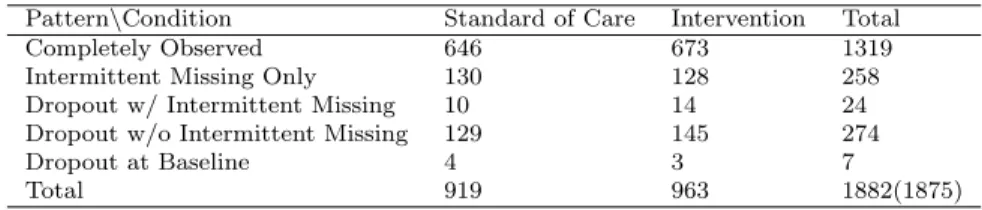
The longitudinal Poisson response variable we considered is the total number of ACASI-reported unprotected penile-vaginal or penile-anal sex acts in the past 4 weeks with part-ners of any HIV status. Therefore, the longitudinal Poisson response variable and the binary response variable are highly correlated. Furthermore, the two types of longitudinal measurements share with the same missing data pattern. We also expect that the longi-tudinal Poisson response variable contains more information than than the longilongi-tudinal binary response variable. Table 2.3 summarizes the missing pattern of the longitudinal count response data (ACASI-reported number of unprotected sex acts) and the number of unprotected sex acts by visit and treatment are visually exhibited in Figure 1.2.
Determining whether missing responses are ignorable or nonignorable is of great prac-tical interest in HIV intervention clinical trials, which greatly motivates our proposed methodology.
Table 1.2: Missing Pattern of the Count Responses (ACASI-reported number of unpro-tected sex acts).
Pattern\Condition Standard of Care Intervention Total
Completely Observed 646 673 1319
Intermittent Missing Only 130 128 258
Dropout w/ Intermittent Missing 10 14 24
Dropout w/o Intermittent Missing 129 145 274
Dropout at Baseline 4 3 7
Figure 1.2: Trellis plots of the count responses (ACASI-reported number of unprotected sex acts).
Number of Unprotected Sex Acts
Count 200 400 600 0 5 10 15 20 534 73 65 43 23 11 9 2 4 1 3 1 5 0 0 0 1 0 0 0 1 Control 18−Month 614 66 53 37 9 7 7 2 3 3 0 0 1 1 1 1 0 0 0 0 0 Intervention 18−Month 550 77 58 46 26 14 14 3 7 1 1 0 2 0 2 0 0 0 0 0 0 Control 12−Month 200 400 600 622 64 61 25 13 5 5 3 2 0 2 0 2 0 0 1 0 0 0 0 0 Intervention 12−Month 200 400 600 518 75 75 44 24 13 10 2 12 7 4 1 1 1 1 0 3 1 0 0 2 Control 6−Month 588 88 75 39 24 9 10 2 2 1 5 0 1 2 0 0 1 0 1 0 0 Intervention 6−Month 383 144140 65 47 17 14 6 16 3 8 2 3 0 1 1 3 1 0 1 2 Control Baseline 0 5 10 15 20 200 400 600 407 150141 81 44 20 27 6 20 3 4 1 12 0 1 2 4 1 0 0 0 Intervention Baseline 1.4 Methodologies Overview
One challenge of the probit mixed-effects regression model for longitudinal binary response data is the estimation of the variances of the random effects. In Chapter 2, we propose a new reparameterization technique to develop a new probit model with latent variables. Our proposed model not only makes the variance for the random effects more identifiable but it also improves convergence and mixing of the Gibbs sampling algorithm, particularly for the parameters involved in the covariance matrix of the random effects. Following Ibrahimet al.(2001, 2005), we adopt a sequence of one-dimensional conditional distributions for the missing data indicators via a logistic regression model, and further show that the posterior distribution is improper if improper uniform priors are specified for the regression coefficients corresponding to the missing binary responses in the logistic
regression models. To overcome this non-identifiability issue, we first specify normal priors for these regression coefficients and then use the DIC and LPML criteria to guide the choice of “optimal” normal priors for the regression coefficients. We further propose a variation of Jeffreys prior, which circumvents the identifiability issue all together. The proposed Jeffreys prior is attractive since it is relatively noninformative, guarantees that the joint posterior distribution is proper, and has similar performance as the “optimal” normal priors. Finally, the proposed joint model for the longitudinal binary responses and the missing data mechanism (ignorable or nonignorable) is computationally attractive since it allows us to conveniently sample missing binary responses and to apply the collapsed Gibbs technique (Liu, 1994) within the Gibbs sampling framework.
For the longitudinal count response data in Chapter 3, we apply the zero-inflated Pois-son model for the response measurements, and propose a new conditional model for the missing data mechanism. The new model has the potential of reducing the number of nuisance parameters, allows us to model dropout and intermittent missing jointly, and provides a broad class of missing data mechanisms, which includes the sequential condi-tional model (Ibrahim et al., 2001, 2005) as one special case. We then investigate and characterize the conditions for propriety of the joint posterior distribution under the new models, and propose a variation of Jeffreys prior as a remedy for impropriety of the pos-terior. In addition, we develop an efficient Gibbs sampling algorithm, which allows us to conveniently sample missing responses and to apply the hierarchical centering technique (Chenet al., 2000) within the Gibbs sampling framework.
1.5 Dissertation Outline
The rest of the thesis is organized as follows. In Chapter 2, we introduce a new probit model with latent variables, and presents a joint multinomial model for the missing data indicators. We then investigate and characterize the conditions for propriety of the joint posterior distribution, followed by a variation of Jeffreys prior as a remedy for impropriety of the posterior. In addition, we develop an efficient Gibbs sampling algorithm, and provide a detailed formulation of the partial DIC and conditional LPML criteria in the presence of missing data. An extensive simulation and a detailed analysis of the HIV prevention behavioral data are carried out in the end of this chapter.
Chapter 3 presents the model for longitudinal Poisson response variable, as well as the new missing data mechanisms for dropouts and intermittent missing. Again, we investigate and characterize the conditions for propriety of the joint posterior distribution, and provide a variation of Jeffreys prior to resolve the improper issue of the posterior. We then conduct the HIV prevention behavioral data analysis, using a new efficient Gibbs sampling algorithm. Extensive real data analyses are conducted in Chapter 4 to assess the performances of missing data mechanism under different scenarios. Future research directions are given in Chapter 5. The proofs of theorems are given in Appendix A. The additional tables are given in Appendix B.
Models for Longitudinal Binary Response Data
2.1 The Proposed Models
Suppose there are a total ofT visits and K health districts in a clinical trial. Let yt
denote the measurement for a patient at visit t in the kth health district (1 ≤ k ≤ K),
and yt = (y0, y1, . . . , yt)0 denote the vector containing all the measurements up to and
including visit t, for t = 0, . . . , T, where y0 represents the baseline measurement. Also,
denote byzthe intervention indicator such thatz= 0 if the subject belongs to the control
arm and z= 1 if the subject belongs to the intervention arm.
2.1.1 The Model for Longitudinal Binary Measurements
According to Verbeke (2005), for longitudinal measurements, it is often assumed thatyt
follows a pre-specified distributionF(β, t), depending on covariates and is parameterized
through a vectorβ, common to all subjects, and subject-specific random effectst. When
yt is binary, the probit mixed-effects regression model is assumed and given by
P(yt= 1|z,x1, k,β∗, τ∗, ζk, ∗t) = Φ(zβ ∗ 1t+x 0 1β ∗ 2t+τ ∗ ζk+∗t), (2.1) 12
for t = 0, . . . , T, where Φ is the N(0,1) cumulative distribution function, x1 is a
vec-tor of baseline covariates, β∗ = (β1∗t,β2∗0t)0 with β1∗t denoting the regression coefficient
corresponding to treatment condition and β∗2t is the vector of regression coefficients cor-responding to x1. Due to the design of the HIV prevention behavioral data that
six-teen health districts were randomized instead of patients, we introduce random effects
ζk i.i.d.
∼ N(0,1) with τ∗2(τ∗ > 0) being the variance, representing the random effect
for all the patients from the kth heath district, k = 1, . . . , K. We further assume that
∗ = (∗0, ∗1, . . . , ∗T)0∼N(0, σ2Σ), where Σ is a (T + 1)×(T + 1) correlation matrix with
(s, t)thentryρ|t−s|. However, under this formulation, the varianceσ2 of the random effects
cannot be estimated.
To better see this identifiability problem, we obtain an equivalent representation of the model given in (2.1) by introducing the latent variablesw∗ = (w∗0, . . . , w∗T). Following
Albert and Chib (1993), (2.1) can be reformulated as
yt= 1 ifw∗t ≥0, 0 ifw∗t <0, (2.2) and w∗t |∗t ∼N(zβ∗1t+x01β∗2t+τ∗ζk+∗t,1) (2.3) fort= 0,1, . . . , T, where∗ = (∗0, ∗1, . . . , ∗T)0 ∼N(0, σ2Σ).
First we note thatyt modeled in (2.2) is invariant with respect to the scale parameter
(variance) of w∗t. To be more specific, if we replacewt∗ in (2.3) by C·wt∗, whereC is any
nonnegative constant, (2.2) is still identical to (2.1). Therefore, the marginal variance of
w∗t as well as the marginal variance of ∗t are not identifiable. Another issue with this
is 1 +σ2, is partially confounded with the scale parameter σ2 in the binary response
model (See Kim et al. (2008) for a related discussion and Remark 2.1). These issues
ultimately imply that β∗ is essentially not identifiable and this leads to poor convergence of the Gibbs sampling algorithm. To circumvent these problems, we consider the following reparameterization: wt= wt∗ √ 1 +σ2, βt= β∗t √ 1 +σ2, τ = τ∗ √ 1 +σ2, t= ∗t √ 1 +σ2. (2.4)
After this reparameterization, we propose our equivalent but identifiable model as
P(yt= 1|z,x1, k,β, τ, ζk, t) = Φ{(zβ1t+x01β2t+τ ζk+t) p 1 +σ2}= π t, (2.5) or yt= 1 ifwt≥0, 0 ifwt<0, (2.6) and wt|t∼N(zβ1t+x01β2t+τ ζk+t, 1 1 +σ2) (2.7) for t = 0,1, . . . , T, where = (0, . . . , T)0 ∼ N(0, σ 2
1+σ2Σ). Under this new model, the marginal variance of wt equals 1, leading to a better separation between β and σ2, and
improving convergence and mixing of the Gibbs sampling algorithm. For simplicity, we let α denote 1+σ2σ2 throughout the remainder of the chapter.
The proposed model is attractive since (i)t captures the dependence of the
longitu-dinal measures, yt, over time; (ii) the time-varying vector of coefficients βt allows us to
assess effectiveness of the intervention over time; (iii) the random effect ζ adjusts for the effects of 16 health districts; and most importantly (iv) all the parameters involved in the model given by (2.5) or the model defined by (2.6) and (2.7) are identifiable.
Remark 2.1: After the reparameterization in (2.4), βt, as the ratio of β
∗
t and
√ 1 +σ2
is now identifiable. This implies that, in the original formulation of (2.3), a large value of σ2 corresponds to large absolute values of the elements in β∗ due to the dual role
σ2 plays in both the binary response and the latent variable model. It thus becomes
difficult to interpret the meaning of β∗, and leads to poor convergence of the Gibbs sampling algorithm. This phenomenon is also empirically observed in our analysis of the HIV data discussed in Section 1.3 by fitting the model defined by (2.2) and (2.3) without reparameterization, which further confirms the necessity of the reparameterization technique.
2.1.2 Missing Data Mechanism
LetRT = (R0, . . . , RT)0 denote the vector of the missing data indicators. The missing
data indicator, Rt, at timet is defined as
Rt= 0 ifyt is observed, 1 ifyt is missing.
DenotingP(Rt= 1|Rt−1,yt, z,x2,γt),Pt, a logistic regression model is assumed for
Pt: logit(Pt) = log Pt 1−Pt =zγ1t+x02γ2t+g(Rt−1,γ3t) +h(yt,γ4t), (2.8)
where x2 is a vector of baseline covariates, which may be different from x1, while g and
h are certain linear functions. We set g = 0 when t = 0 since there are no previous
missing indicators (Rt−1). Following Ibrahim et al. (1999, 2005), we construct the joint
distribution of R via a sequence of one-dimensional conditional distributions,
P(R0 =r0, . . . , Rt=rt|yt, z,x2,γ) = T
Y
t=0
Remark 2.2: If we assume thatP(Rt=m|Rt−1 =l,yt, z,x2,γt) depends on the
longitu-dinal measures only through the current and previous visits, we simply take h(yt,γ4t) =
γ4t1yt−1+γ4t2yt in (2.8). The model in (2.9) implies nonignorable missingness due to the
existence of intermittent missingness and dropout. We may also let h(yt,γ4t) = 0 if the
missingness is ignorable. (See Section 2.4 for further discussion.)
Remark 2.3: For t >0, we may choose g(Rt−1,γ3t) =R0t−1γ3t, which depends on all of
the previous missingness indicators. In this chapter, we set g(Rt−1,γ3t) =
Pt−1
j=0Rjγ3t.
The new covariate Pt−1
j=0Rj captures the cumulative number of missing response
indica-tors, reduces the number of nuisance parameters for modeling the missing data mechanism, and makes the nonignorable missing data mechanism more identifiable (See Section 2.2.2).
2.2 Bayesian Inference
2.2.1 The Likelihood Function
Suppose there arensubjects and assume that (zi, ki,x1i,x2i) are completely observed,
for all i = 1, . . . , n. Let yobs = (y10,obs, . . . ,y
0 n,obs) 0 and y mis = (y01,mis, . . . ,y 0 n,mis) 0, where
(yi,obs,yi,mis) are the observed and missing binary responses for the ith subject.
Let yi = (yi0, . . . , yiT), and RiT denote the collection of all missing data indicators
RiT = (Ri0, . . . , RiT). Denote by Dc = {yi, zi, ki,x1i,x2i, ζki,i,wi,Ri, i = 1, . . . , n}
the set of complete data and Dobs = {yi,obs, zi, ki,x1i, x2i,Ri, i = 1, . . . , n} is the set of
observed data. Denote by fy andfR the marginal densities ofy andR, respectively. Let
Let [A|B] denote the conditional distribution of A given B. We model the observed
data through the sequence of conditional distributions [y][R|y]. The complete data like-lihood function is therefore given by
L(θ|Dc) = n Y i=1 fy(yi|zi,x1i, ki, ζki,i,wi,θ)fR|y(RiT|yi, zi,x2i,θ) = n Y i=1 T Y t=0 1(wit≥0)yit1(wit <0)1−yit 1 p 2π(1−α) exp{−(wit−ziβ1t−x 0 1iβ2t−τ ζki −it) 2 2(1−α) } Pit1(rit=1)(1−Pit)1(rit=0) 1 √ 2π exp − ζk2 i 2 ! 1 p 2π|αΣ|exp − 1 2α 0 iΣ−1i . (2.10)
After integrating out the missing longitudinal responses yi,mis, ζki, i, and the latent
variables wi, the observed data likelihood function is given by
L(θ|Dobs) =X ymis Z n Y i=1 T Y t=0 1(wit≥0)yit1(wit<0)1−yit 1 p 2π(1−α)exp{− (wit−ziβ1t−x10iβ2t−τ ζki−it) 2 2(1−α) }dwPit 1(rit=1)(1−P it)1(rit=0) 1 √ 2πexp − ζk2 i 2 ! dζ 1 p 2π|αΣ|exp − 1 2α 0 iΣ −1 i d. (2.11)
2.2.2 Prior and Posterior Distributions
We assume that the joint prior density can be expressed as
π(θ) =π(β)π(γ)π(α)π(τ)π(ρ).
The joint posterior based on the observed data Dobs is written as
π(θ|Dobs)∝ L(θ|Dobs)π(θ). (2.12)
We first establish a useful proposition regarding the propriety of the posterior distri-bution when an improper uniform prior is assumed for γ.
Proposition 2.2.1. Suppose we take π(γ)∝1, the joint posterior in (2.12) is improper
regardless of whether π(β, α, τ, ρ) is proper or improper.
A sketch of the proof of the proposition is given in Appendix A. From Proposition 2.2.1, the joint posterior distribution is improper if π(γ) ∝ 1. The next proposition, based on
Chen and Shao (2001), states that under some mild conditions, the joint posterior is proper ifπ(γ) is proper, butπ(β, α, τ, ρ)∝1.
LetZi be the (T + 1)×(T+ 1) diagonal matrix with diagonal element being zi,X1i
is the matrix with all the row vectors equal x01i, and β = (β01, . . . ,β0T)0 is a vector of
lengthp. Denote byIc={i|Ri0 = 0, . . . , RiT = 0}the set of observations with no missing
visits, and ˜i = (i−1)(T + 1) + (t+ 1), for 1 ≤ i≤ n, 0 ≤ t ≤T. Let = (0i, i ∈ Ic)0,
ui = (ui0, . . . , ui,T)0, u = (ui0, i ∈Ic)0, where the uit’s are i.i.d N(0,1) random variables.
LetX∗ ={(Zi,X1i)0, i∈Ic}0 be the design matrix, where each row vector is defined asx0i.
We further introduceX∗obs to be the matrix with rows equal (1−yit)x
0
˜i, such thati∈Ic.
Proposition 2.2.2. Suppose we take π(γ) to be a proper prior, letπ(τ) be a proper prior
with a finite pth moment, and specify improper uniform priors for the other parameters.
The joint posterior in (2.12) is proper if the following conditions are satisfied: (C1) X∗ is of full rank; and (C2) there exists a positive vector a, i.e., each component ai >0, such
that X∗obs0a= 0.
Next, we consider Jeffreys prior (Jeffreys, 1946) regardingγ. Due to the involvement of the missing data in the design matrix, the conventional Jeffreys prior is computationally infeasible. However, we observe that Jeffreys prior based on a certain subset of the data is not only computationally feasible, but also leads to a proper posterior distribution (Chen et al., 2008). Thus, we propose a variation of Jeffreys prior, which is analytically
attractive. To be specific, we select a certain observed subset, denoted by ˜Dobs, such that
the likelihood function of the parameters does not involve any missing data. The logarithm of the joint likelihood function in (2.11) based on ˜Dobs is given by
`(θ|D˜obs) = log Z Y (i,t)∈D˜obs 1(wit≥0)yit1(wit<0)1−yit 1 p 2π(1−α)exp{− (wit−ziβ1t−x10iβ2t−τ ζki −it) 2 2(1−α) }dw 1 √ 2π exp − ζk2 i 2 ! dζp 1 2π|αΣ|exp − 1 2α 0 iΣ −1 i d + log Y (i,t)∈D˜obs Pit1(rit=1)(1−Pit)1(rit=0). (2.13)
For γt at visit t, we use a different observed subset to construct the prior, aiming to
utilize as many observations as possible. Indeed, the idea of using a subset of the data is equivalent to selecting the corresponding terms from the log-likelihood function. That is, if we takeh(yt,γ4t) =γ4tytfort= 0, andh(yt,γ4t) =γ4t1yt−1+γ4t2ytfort >0 in (2.8),
the log-likelihood of γt based on this subset of the data is given by
`(γt|Dc) = Pn i=1log Pit1(rit=1)(1−Pit)1(rit=0) 1(rit=0) t= 0, Pn i=1log Pit1(rit=1)(1−Pit)1(rit=0) 1(rit−1=0)1(rit=0) t >0, = Pn i=11(rit = 0) log(1−Pit) t= 0, Pn i=11(rit−1 = 0)1(rit= 0) log(1−Pit) t >0. We now specify the joint prior distribution for γt as
π(γt)∝|X∗t0DtX∗t|1/2, (2.14) where X∗t = 1(rit = 0)X∗it:i= 1, . . . , n 0 t= 0, 1(rit−1 = 0)1(rit= 0)X∗it:i= 1, . . . , n 0 t >0,
|.| represents the determinant of a matrix, X∗it = (z,x02,yit)0 if t = 0, and X∗it = (z,x02,
Pt−1
j=0Rj,yit−1,yit)0 fort >1. Fort= 1, since Ptj−=01Rj =R0= 0 for the subjects within
this subset, an improper uniform prior is essentially assumed for γ3t in π(γt) defined
by (2.14) while Jeffreys prior is constructed for the other parameters in γt such that
X∗it = (z,x02,yit−1,yit)0. Also, in (2.14), Dt is an n×n diagonal matrix with diagonal
elements being Pit(1−Pit). If the design matrix X∗t is of full column rank (Chen et al.,
2008), the prior for the corresponding parameters in γtis proper. In addition, we specify improper uniform priors for (β, α, ρ), and a truncated normal prior forτ.
2.2.3 Computational Development
The joint posterior distribution of (θ,ymis) based on the observed data is given by
π(θ,ymis|Dobs)∝ L(θ|Dc)π(θ), (2.15)
where L(θ|Dc) is defined in (2.10). Thus, the joint posterior distribution of (β,γ, α, τ, ρ)
is written as π(β,γ, α, ρ, τ,ymis,w,ζ,,|Dobs) ∝ n Y i=1 T Y t=0 1(wit ≥0)yit1(wit<0)1−yitPit1(rit=1)(1−Pit)1(rit=0) (1−α)−n(T+1)/2 n Y i=1 T Y t=0 exp −(wit−ziβ1t−x 0 1iβ2t−τ ζki −it) 2 2(1−α) n Y i=1 T Y t=0 exp −ζ 2 ki 2 ! (α)−n(T+1)/2 n Y i |Σ|−1/2exp − 1 2α 0 iΣ −1 i π(β)π(γ)π(α)π(τ)π(ρ). (2.16)
The Gibbs sampling algorithm requires sampling from the following full conditional distributions in turn:
(i) [ymis,γ|w,β,ζ,, α, τ, ρ, Dobs]; (ii) [w,β|ymis,γ,ζ,, α, τ, ρ, Dobs];
(iii) [α, ρ|ymis,w,β,γ,ζ,, τ, Dobs]; (iv) [|ymis,w,β,γ,ζ, α, τ, ρ, Dobs];
(v) [τ|ymis,w,β,γ,ζ,, α, ρ, Dobs]; (vi) [ζ|ymis,w,β,γ,, α, τ, ρ, Dobs]. (2.17)
For (i), we first collapse out the latent random variablesw via the following identity:
[ymis,γ,w,β|ζ,, α, τ, ρ, Dobs] = [ymis,γ|β,ζ,, α, τ, ρ, Dobs][w,β|ymis,γ,ζ,, α, τ, ρ, Dobs]
= [ymis|β,γ,ζ,, α, τ, ρ, Dobs][γ|ymis, Dobs][w,β|ymis,γ,ζ,, α, τ, ρ, Dobs], (2.18)
and then run a sub-Gibbs sampling algorithm to sample from the following full conditional distributions in turn: (ia)[ymis|β,γ,ζ,, α, τ, ρ, Dobs] and (ib)[γ|ymis, Dobs].
Sampling w and β in (ii) are straightforward since the components of w are condi-tionally independent truncated normal random variables, and β, conditional on the other parameters and variables, follows a multivariate normal distribution.
The posterior distribution of (α, ρ) in the binary response model is highly dependent
on the random effects . Directly sampling (α, ρ) from their full conditional distributions
will lead to slow convergence and poor mixing of the Gibbs sampling algorithm. Due to the introduction of the probit link and the latent variables w, we are able to analytically integrate out . For (iii), we again apply the collapsed Gibbs technique through the identity:
[α, ρ,|ymis,w,β,γ,ζ, τ, Dobs] = [α, ρ|ymis,w,β,γ,ζ, τ, Dobs][|ymis,w,β,γ,ζ, α, τ, ρ, Dobs].
Sampling in (iv) is also straightforward since the t are independent multivariate normal random variables conditional on the other parameters and variables.
Below, we briefly explain how to sample from these full conditional distributions.
Step (ia). For each missing response yit,mis, we compute qit as
qit= πit T0 Y j=t P(rij|rij−1,yij, yit= 1, z,x2,γ)+ (1−πit) T0 Y j=t P(rij|rij−1,yij, yit= 0, z,x2,γ) −1 πit T0 Y j=t P(rij|rij−1,yij, yit = 1, z,x2,γ),
where T0 = min(t+ 1, T), it refers to the tth visit for the ith observation, πit is
introduced in (2.5), and P(rij|rij−1,yij, z,x2,γ) is given in (2.8). We next sample
yit from a Bernoulli(qit) distribution.
Step (ib). We write the full conditional distribution ofγ as
π(γt|ymis, Dobs)∝ n Y i=1 P1(rit=1) it (1−Pit)1(rit=0)π(γt),
where Pit is established in (2.8). Let π(γ) be the Jeffreys prior constructed in
Section 2.2.2. We cannot use adaptive rejection sampling since Jeffreys prior is not log-concave (Chen et al., 2008). Thus, we use the localized Metropolis algorithm to sample γ.
Step (iia). We simply draw wit from a truncated N(ziβ1t+x01iβ2t+τ ζki +it,1−α)
distribution given yit, fori= 1, . . . , n, and t= 0, . . . , T.
Step (iib). Let ˜Xi = (zi,x01i)0. Assumingπ(βt)∝1, we sampleβt|ymis,w,ζ,, α, τ, ρ, Dobs
fort= 0, . . . , T from N n X i=1 ˜ X0iX˜i −1 n X i=1 ˜ X0i(wit−τ ζki−it), n X i=1 ˜ X0iX˜i −1 (1−α) .
Step (iii). Letµ1i= (wi0−ziβ10−x10iβ20−τ ζki, . . . , wiT −ziβ1T −x
0
1iβ2T −τ ζki)
0 and
Σ1−1 = α1Σ−1+1−1αI. The joint full conditional distribution [α, ρ|ymis,w,β,γ,ζ,, τ,
Dobs] is given by π(α, ρ|ymis,w,β,γ,ζ,, τ, Dobs) ∝ {α(1−α)}−n(T2+1)|Σ|− n 2π(α)π(ρ) n Y i=1 exp− 0 i(α1Σ −1+ 1 1−αI)i− 2 1−αµ 0 1ii+1−1αµ 0 1iµ1i 2 ∝ {α(1−α)}−n(T2+1)|Σ|− n 2π(α)π(ρ) n Y i=1 exp( 1 (1−α)2µ 0 1iΣ1µ1i−1−1αµ 0 1iµ1i 2 ) n Y i=1 exp − (i− 1 1−αΣ1µ1i) 0Σ 1−1(i−1−1αΣ1µ1i) 2 .
We next integrate out , and the joint full conditional distribution simplifies to
π(α, ρ|ymis,w,β,γ,ζ, τ, Dobs) ∝ {α(1−α)}−n(T2+1)|Σ|− n 2|Σ1| n 2 n Y i=1 exp( 1 (1−α)2µ 0 1iΣ1µ1i−1−1αµ 0 1iµ1i 2 )π(α)π(ρ).
(a). The full conditional distribution of α is given by
π(α|ymis,w,β,γ,ζ, τ, ρ, Dobs)∝ {α(1−α)} −n(T2+1)|Σ 1| n 2 n Y i=1 exp( 1 (1−α)2µ01iΣ1µ1i−1−1αµ01iµ1i 2 )π(α).
Since α is always between 0 and 1 exclusively, we introduceδ such that
α= 1 1 +e−δ
with support on (−∞,∞) to indirectly sample α. Thus
π(δ|ymis,w,β,γ,ζ, τ, ρ, Dobs) =π(α|ymis,w,β,γ,ζ, τ, ρ, Dobs)
eδ
Under a uniform prior specified for α, we use the localized Metropolis algorithm to
sample δ, and then convert it back toα.
(b). The full conditional distribution ofρ is given by
π(ρ|ymis,w,β,γ,ζ, α, τ, Dobs)∝ |Σ| −n 2|Σ1| n 2 n Y i=1 exp( 1 (1−α)2µ 0 1iΣ1µ1i 2 )π(ρ).
Since −1 < ρ < 1, we use a “de-constraining” transformation to sample ρ (Chen
et al., 2000):
ρ= −1 +e ξ
1 +eξ −∞< ξ <∞.
Thus
π(ξ|ymis,w,β,γ,ζ, α, τ, Dobs) =π(ρ|ymis,w,β,γ,ζ, α, τ, Dobs) 2eξ
(1 +eξ)2.
Assume that a Uniform(−1,1) prior is specified forρ. Sinceπ(ξ|,β, α,ymis, Dobs) is
not log-concave, we again use the localized Metropolis algorithm to sample ξ, and
then convert it back to ρ.
Step (iv). Based on the derivation in Step (iii), draw i from aN
1
1−αΣ1µ1i,Σ1
.
Step (v). The full conditional distribution of τ is given by
π(τ|ymis,w,β,γ,ζ,, α, ρ, Dobs) ∝exp ( − Pn i=1 PT t=0(wit−ziβ1t−x01iβ2t−τ ζki−it) 2 2(1−α) ) π(τ).
Assume τ follows the truncated normal priorτ ∼N(0,10)1(τ >0). We then draw
τ from the posterior distribution
N Pn i=1 PT t=0ηitζki Pn i=1 PT t=0ζki2 1−α + 1 10 , Pn 1 i=1 PT t=0ζki2 1−α + 1 10 1(τ >0), where ηit=wit−ziβ1t−x01iβ2t−it.
Step (vi). The full conditional distribution of ζk is given by π(ζk|ymis,w,β,γ,, α, τ, ρ, Dobs) ∝exp ( − P {i|ki=k} PT t=0(wit−ziβ1t−x01iβ2t−τ ζki−it) 2 2(1−α) ) exp − P {i|ki=k} PT t=0ζk2i 2 ! .
We then draw ζk from a N
P {i|ki=k} PT t=0ηit1−τα nk(T+1) τ 2 1−α+nk(T+1) , 1 nk(T+1) τ 2 1−α+nk(T+1) distribution fork= 1, . . . ,16, wherenk is the total number of patients in thekthhealth district,
i.e., nk=P{i|ki=k}1.
2.2.4 Bayesian Model Assessment
It is of great practical interest to try to assess whether the missingness is ignorable or nonignorable. In this section, several Bayesian model assessment criteria are considered, namely, the DIC relating to the missing data model (DICR|y)(Yao et al., 2015; Mason
et al., 2012), and the LMPL relating to the missing data model (LPMLR|y) (Zhanget al.,
2014a).
Since our focus is on the missing data mechanism, these criteria are applied only to the distribution of the missing data indicators. Both criteria are computationally attractive, and can be implemented with any types of priors, i.e., informative, noninformative, or even improper priors.
DICR|y. Let ψ = (γ,ymis) denote the vector of the missing data model parameters
of interest, where we view ymis as nuisance parameters. For the missing model in (2.8),
D(ψ) =−2Pn i=0
PT
t=0[ritηitr−log(1+exp(ηrit))]. For computingD(ψ), we need to estimate
several discrete parameters such as the binary response ymis. The posterior mean of ymis, which is no longer binary, may not be a desirable estimate to be applied in the DICR|y
formula. Instead, we may use the posterior mode, which maintains the binary nature of these parameters. Another possible choice given in Huang et al. (2005) is that we apply the linear predictor ηitr directly to the DICR|y formula. Therefore, we have DICR|y =
D(ηr) + 2p
D, whereηitr =E[ziγ1t+x02iγ2t+g(Rit−1,γ3t) +h(yit,γ4t)|Dobs],pD =D(ψ)−
D(ψ) is the effective number of parameters in the model, and D(ψ) = E[D(ψ)|Dobs].
This modification is appropriate since the model for the missing data indicators depends on ψ only through the linear predictor ηr. Moreover, with the introduction of ηr in the computation of DICR|y, we no longer need to worry about the discreteness of the
parameters since ηr is always continuous. Similar to the traditional DIC, the model with the smallest DICR|y value is the most optimal among all the models under consideration.
LPMLR|y. To assess the missing data mechanism, we adopt the conditional LPML
(Hansonet al., 2011), where the pseudomarginal probability, i.e.,Qn
i=1P(RiT|yi, zi,xi,γ),
is used to quantify the model’s predictive ability. Let Dobs(−i∗) ={RjT, j= 1, . . . , i−1, i+
1, . . . , n} ∪ {(yj,obs, zj,xj), j = 1, . . . , n} denote the observed data with RiT deleted. Let
ψ1 = (β, τ,ζ, α, ρ), and ψ= (ψ1,γ). Then we have
π(ψ,ymis,|D (−i∗) obs )∝ n Y j=1 fy(yj|ψ, zj,xj,j)f(j|α, ρ) ×Y j6=i fR|y(RjT|γ,yj, zj,xj)π(ψ).
The simplified conditional predictive ordinate CPOi (Chen et al., 2000; Hanson et al., 2011) can be written as CPOi = Z X yi,mis fR|y(RiT|γ,yi, zi,xi)π(ψ,ymis,|D (−i∗) obs )ddψ = R P 1 ymis 1 fR|y(RiT|γ,yi,zi,xi)π(ψ,ymis,|Dobs)ddψ ,
and the logarithm of the pseudomarginal likelihood is given by LPMLR|y = n X i=1 log(CPOi).
Let{(ψb,ymis,b,b), b= 1, . . . , B}denote a Gibbs sample of (ψ,ymis,) from (2.15) and let
b represent the bth iteration. A Monte Carlo estimate of CPO
i is given by CPOi = 1 B B X b=1 1
fR|y(RiT|yi,obs, zi,xi,ψb,yi,mis,b,i,b)
!−1 .
Similar to the conventional LPML, a large value of LPMLR|y indicates a more favorable
model.
2.3 A Simulation Study
In this section, we conduct a simulation study to investigate the empirical performance of the proposed method. In the data generation, we first generated n= 2000 baseline
co-variates as follows: x1i ∼ N(0,1), x2i|x1i ∼ Bernoulli(1/(1 + exp(−0.2−0.2x1i))), and
the intervention indicator zi ∼Bernoulli(0.5). Similar to the HIV prevention behavioral
data, we set the total number of visits equal 4. Let ∗ in (2.1) follow a N(0, σ2Σ)
distri-bution, whereσ2 = 2 (α≈0.667) and Σ is a 4×4 AR(1) correlation matrix withρ= 0.8.
The longitudinal binary response variable yit was generated from a Bernoulli distribution
with the probability of yit= 1 given by
where β∗t = (β0∗t, β1∗t, β2∗t, β3∗t)0 for t = 0,1,2,3. To reproduce the longitudinal binary
response data pattern of the HIV prevention behavioral data, we set
β∗00 β∗10 β∗20 β∗30 = −1.0 0.5 1.0 0.4 −1.0 0.5 1.0 −0.2 −1.0 0.5 1.0 −0.4 −1.0 0.5 1.0 −0.6 . (2.20)
We then generated the missing data indicatorRit∼Bernoulli(Pit), where Pit is given by
logit(Pit) =γ0t+x1iγ1t+x2iγ2t+ziγ3t+ t−1
X
j=0
Rijγ4t+yit−1γ5t+yitγ6t. (2.21)
The missing data mechanism is, therefore, nonignorably missing sincePitin (2.21) depends
on the unobserved datayit−1 andyit whenRi,t−1 =Rit = 1. Letγt= (γ0t, γ1t, γ2t, γ3t, γ4t,
γ5t, γ6t)0 fort= 0,1,2,3. We set γ00 γ10 γ20 γ30 = −2.50 0.50 −0.50 −0.50 0.00 0.00 0.00 −2.00 0.50 −0.50 −0.25 −0.25 0.50 0.40 −2.80 0.50 −0.50 0.25 −0.60 1.30 1.70 −2.80 0.50 −0.50 0.50 0.60 −0.50 1.70 . (2.22)
Under this setting, the average missingness percentages across the 250 simulated data sets were 5.37%, 10.52%, 11.94%, and 14.18% at t= 0,1,2,3, respectively.
To further examine the performance of the proposed method, we also considered an-other scenario, in which the missingness percentage of the last visit (t = 3) was set to
47.14% and the missingness percentages at the other time points remained the same. This was achieved by setting γ03 in (2.22) equal -0.50. In the simulation, we assigned the
true values to the initial values for each parameter. After discarding the first 500 itera-tions of the sampler, we used the subsequent 5,000 iteraitera-tions for computing the posterior summaries.
We fit both the ignorable and nonignorable models to the simulated data generated from the nonignorable model. For the ignorable model, we set γ5t and γ6tin (2.21) equal
0 so that Pit depends only on the intervention indicator, the covariates x2, as well as the
cumulative number of missing visits, which all were observed. For the nonignorable model, we considered Jeffreys prior for γt in (2.14), as well as a N(0, σ2prior) prior for γ6t, where
σ2prior= 1,2, . . . ,10.
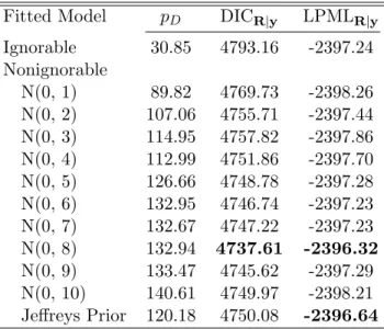
When the missingness percentage was low (similar to the real data), the median (IQR) of DICR|y under the ignorable model was 4562.49 (4490.64, 4641.60). The nonignorable
model with a N(0, 10) prior had the smallest median value of DICR|y (4473.76 (4381.28,
4465.02)). The median (IQR) of LPMLR|y under the ignorable model was -2281.40
(-2320.90, -2245.39). Among all the normal priors, the nonignorable model with a N(0, 6) prior had the largest median value of LPMLR|y (-2273.04 (-2313.26, -2234.85)), and
the nonignorable model with the Jeffreys prior had the largest value (-2272.85 (-2311.38, -2235.87)) of LPMLR|y among all the models under consideration.
For the high missingness percentage scenario (47.14% missing at the last visit), the median (IQR) of DICR|y under the ignorable model was 5673.07 (5605.66, 5741.60). The
nonignorable model with a N(0, 10) prior still had the smallest median value of DICR|y
(5559.20 (5471.43, 5644.64)). The median (IQR) of LPMLR|y under the ignorable model
was -2836.63 (-2870.99, -2802.92). Among all the normal priors, the nonignorable model with a N(0, 8) prior had the largest median value of LPMLR|y (-2816.79 (-2858.90,
-2781.31)), and the nonignorable model with the Jeffreys prior had the largest value (-2815.01 (-2849.76, -2780.99)) among all the models under consideration.
Let the “DIC Difference” be the DICR|y under the nonignorable model minus the
−400 −200 0 1 2 3 4 5 6 7 8 9 10 Jeffreys σprior2 DIC Diff erence −25 0 25 50 75 1 2 3 4 5 6 7 8 9 10 Jeffreys σprior2 LPML Diff erence (a) (b) −400 −200 0 1 2 3 4 5 6 7 8 9 10 Jeffreys σprior2 DIC Diff erence −25 0 25 50 75 1 2 3 4 5 6 7 8 9 10 Jeffreys σprior2 LPML Diff erence (c) (d)
Figure 2.1: Plots of the DIC differences (a) and the LPML differences (b) when the missingness percentages were 5.37%, 10.52%, 11.94%, and 14.18%; and plots of the DIC differences (c) and the LPML differences (d) when the missingness percentages were 5.37%, 10.52%, 11.94%, and 47.14%.
under the nonignorable model minus the LPMLR|yunder the ignorable model. Figure 2.1
shows the plots of the DIC differences and the LPML differences versus different priors (N(0, σ2prior)’s or Jeffreys) specified under the nonignorable model under the two scenarios
with different missingness percentages. From Figure 2.1, we see that (i) the DIC differences first decrease and then slightly increase asσprior2 increases (Figure 2.1(a) and Figure 2.1(c));
and (ii) the LPML differences first increase and then slightly decrease as σprior2 increases
(Figure 2.1(b) and Figure 2.1(d)) under both scenarios. Based on Figure 2.1(a) and Figure 2.1(b), when the missingness percentage is low, the nonignorable model withN(0,6)
seemed to have the best relative performance. For the high missingness percentage case (Figure 2.1(c) and Figure 2.1(d)), the nonignorable model withN(0,9) tended to perform
comparatively better. Moreover, all of the boxes for the “DIC Difference” were below 0, and all of the boxes for the “LPML Difference” were above 0, indicating that both DICR|y
and LPMLR|y were in favor of the nonignorable model over the ignorable model. Also,
as the missingness percentage increases, the boxes for both “DIC Difference” and “LPML Difference” became further away from the horizontal line (y= 0), implying that the power
of the two criteria increased as the missingness percentage increased.
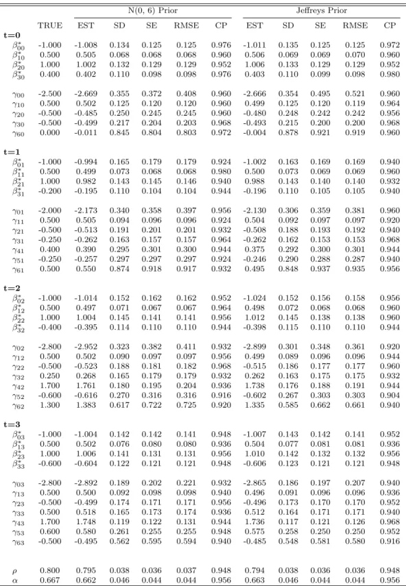
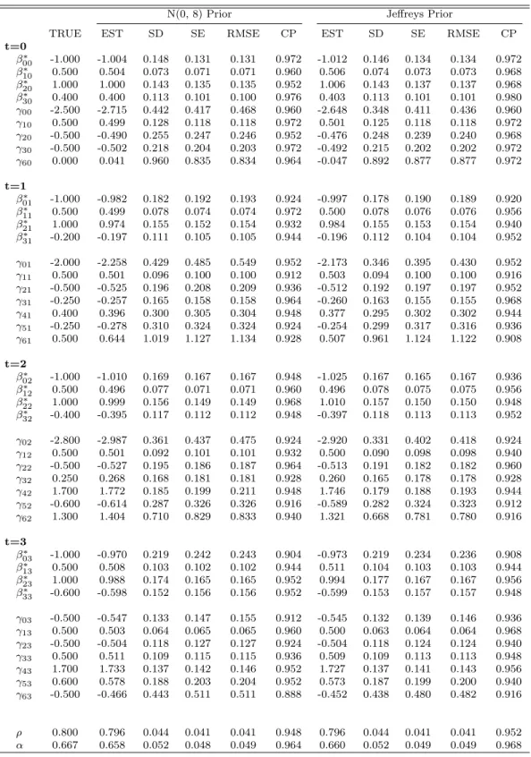
Tables 2.1 and 2.2 show the true value of the parameter (True), the posterior mean (Est), the standard deviation of the estimate (SD), the average of the posterior standard deviations (SE), the root of the mean squared error of the posterior mean (RMSE), and the coverage probability (CP) of the 95% highest posterior density (HPD) interval for each parameter across 250 simulations under the nonignorable models with the N(0,6) prior
and Jeffreys prior for the low missingness percentage case and the nonignorable models with theN(0,8) prior and Jeffreys prior for the high missingness percentage case. We see
SDs, SEs, and RMSEs were close to each other; and (iii) CPs for most of the parameters were approximately 95%, except for some of theγ5tandγ6t. The posterior estimates under
the other priors are given in Tables B.1 and B.2 in the Supplemental Materials. From these tables, we see that the posterior estimates were quite robust to the specification of the N(0, σ2prior) prior under the nonignorable model.
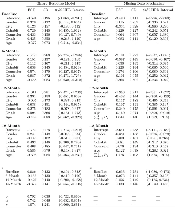
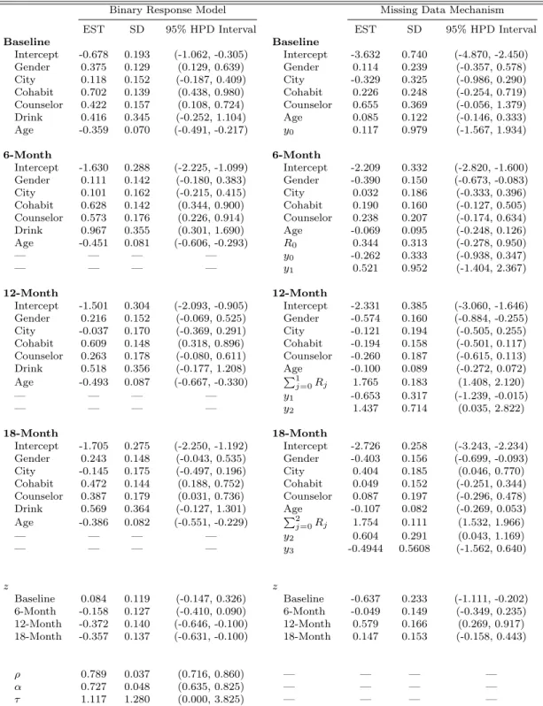
2.4 Analysis of the HIV Prevention Behavioral Data
In this section, we carry out a detailed analysis of the HIV prevention behavioral data discussed in Section 1.3. The baseline covariates in the response model and missing data mechanism include Gender (1=female), City (1=Lives in city or township), Cohabit (1=Cohabitates with sex partner), Counselor (1=Meets with a counselor at least every 3 months), Drink (1=Reported drinking alcohol weekly or more frequently), and Age. Except for Age, which is continuous, all other covariates are binary. Due to the rare events of Drink in the “missing” group of patients, the Drink covariate is not identifiable, and is therefore excluded in the missing data mechanism. For the missing data mechanism, we also consider covariatesyt, andPtj−=01Rjat thetthvisit. For the HIV prevention behavioral
data, we have K = 16 health districts and T = 3, where t = 0 denotes “baseline”, and
visits t = 1 to t = 3 correspond to the three follow-up visits at 6, 12, and 18 months.
The continuous covariate Age was standardized for numerical stability in the posterior computations.
In all the Bayesian computations, we used 20,000 MCMC samples, which were taken from every fifth iteration, after a burn-in of 10,000 iterations for each model to compute all posterior summaries, including posterior means (ESTs), posterior standard deviations (SDs), 95% HPD intervals, DIC, and LPML. The code was written in FORTRAN 95
Table 2.1: Posterior Summaries under the Nonignorable Model with a N(0, 6) Prior and Jeffreys Prior When the Missingness Percentages Were 5.37%, 10.52%, 11.94%, and 14.18%
N(0, 6) Prior Jeffreys Prior
TRUE EST SD SE RMSE CP EST SD SE RMSE CP
t=0 β∗00 -1.000 -1.008 0.134 0.125 0.125 0.976 -1.011 0.135 0.125 0.125 0.972 β∗ 10 0.500 0.505 0.068 0.068 0.068 0.960 0.506 0.069 0.069 0.070 0.960 β∗ 20 1.000 1.002 0.132 0.129 0.129 0.952 1.006 0.133 0.129 0.129 0.952 β∗30 0.400 0.402 0.110 0.098 0.098 0.976 0.403 0.110 0.099 0.098 0.980 γ00 -2.500 -2.669 0.355 0.372 0.408 0.960 -2.666 0.354 0.495 0.521 0.960 γ10 0.500 0.502 0.125 0.120 0.120 0.960 0.499 0.125 0.120 0.119 0.964 γ20 -0.500 -0.485 0.250 0.245 0.245 0.960 -0.480 0.248 0.242 0.242 0.956 γ30 -0.500 -0.499 0.217 0.204 0.203 0.968 -0.493 0.215 0.200 0.200 0.968 γ60 0.000 -0.011 0.845 0.804 0.803 0.972 -0.004 0.878 0.921 0.919 0.960 t=1 β∗ 01 -1.000 -0.994 0.165 0.179 0.179 0.924 -1.002 0.163 0.169 0.169 0.940 β∗11 0.500 0.499 0.073 0.068 0.068 0.980 0.500 0.073 0.069 0.069 0.960 β∗21 1.000 0.982 0.143 0.145 0.146 0.940 0.988 0.143 0.140 0.140 0.932 β∗31 -0.200 -0.195 0.110 0.104 0.104 0.944 -0.196 0.110 0.105 0.105 0.940 γ01 -2.000 -2.173 0.340 0.358 0.397 0.956 -2.130 0.306 0.359 0.381 0.960 γ11 0.500 0.505 0.094 0.096 0.096 0.924 0.504 0.092 0.097 0.097 0.920 γ21 -0.500 -0.513 0.191 0.201 0.201 0.932 -0.508 0.188 0.193 0.192 0.940 γ31 -0.250 -0.262 0.163 0.157 0.157 0.964 -0.262 0.162 0.153 0.153 0.968 γ41 0.400 0.390 0.295 0.301 0.300 0.944 0.375 0.292 0.300 0.301 0.944 γ51 -0.250 -0.257 0.297 0.297 0.297 0.924 -0.246 0.290 0.288 0.287 0.940 γ61 0.500 0.550 0.874 0.918 0.917 0.932 0.495 0.848 0.937 0.935 0.956 t=2 β∗ 02 -1.000 -1.014 0.152 0.162 0.162 0.952 -1.024 0.152 0.156 0.158 0.956 β∗ 12 0.500 0.497 0.071 0.067 0.067 0.964 0.498 0.072 0.068 0.068 0.960 β∗22 1.000 1.004 0.145 0.141 0.141 0.956 1.012 0.145 0.138 0.138 0.960 β∗32 -0.400 -0.395 0.114 0.110 0.110 0.944 -0.398 0.115 0.110 0.110 0.944 γ02 -2.800 -2.952 0.323 0.382 0.411 0.932 -2.899 0.301 0.348 0.361 0.920 γ12 0.500 0.502 0.090 0.097 0.097 0.956 0.499 0.089 0.096 0.096 0.944 γ22 -0.500 -0.523 0.188 0.181 0.182 0.968 -0.515 0.186 0.177 0.177 0.960 γ32 0.250 0.268 0.165 0.179 0.179 0.932 0.262 0.163 0.175 0.175 0.932 γ42 1.700 1.761 0.180 0.195 0.204 0.936 1.738 0.176 0.188 0.191 0.944 γ52 -0.600 -0.616 0.270 0.316 0.316 0.916 -0.602 0.267 0.303 0.303 0.904 γ62 1.300 1.383 0.617 0.722 0.725 0.920 1.335 0.585 0.662 0.661 0.940 t=3 β∗03 -1.000 -1.004 0.142 0.142 0.141 0.948 -1.007 0.143 0.142 0.141 0.952 β∗13 0.500 0.502 0.076 0.080 0.080 0.936 0.504 0.077 0.081 0.081 0.936 β∗ 23 1.000 1.006 0.141 0.131 0.131 0.956 1.010 0.142 0.132 0.132 0.956 β∗33 -0.600 -0.604 0.122 0.121 0.121 0.948 -0.606 0.123 0.121 0.121 0.948 γ03 -2.800 -2.892 0.189 0.202 0.221 0.932 -2.865 0.186 0.197 0.207 0.940 γ13 0.500 0.500 0.092 0.098 0.098 0.940 0.496 0.091 0.096 0.096 0.936 γ23 -0.500 -0.499 0.174 0.171 0.171 0.956 -0.496 0.173 0.170 0.170 0.952 γ33 0.500 0.518 0.165 0.173 0.174 0.936 0.512 0.164 0.171 0.171 0.940 γ43 1.700 1.748 0.119 0.122 0.131 0.944 1.736 0.117 0.121 0.126 0.968 γ53 0.600 0.580 0.261 0.255 0.255 0.948 0.575 0.258 0.250 0.250 0.952 γ63 -0.500 -0.495 0.562 0.595 0.594 0.940 -0.485 0.548 0.581 0.580 0.916 ρ 0.800 0.795 0.038 0.036 0.037 0.948 0.794 0.038 0.036 0.036 0.948 α 0.667 0.662 0.046 0.044 0.044 0.956 0.663 0.046 0.044 0.044 0.956
Table 2.2: Posterior Summaries under the Nonignorable Model with a N(0, 8) Prior and Jeffreys Prior When the Missingness Percentages Were 5.37%, 10.52%, 11.94%, and 47.14%
N(0, 8) Prior Jeffreys Prior
TRUE EST SD SE RMSE CP EST SD SE RMSE CP
t=0 β∗ 00 -1.000 -1.004 0.148 0.131 0.131 0.972 -1.012 0.146 0.134 0.134 0.972 β∗ 10 0.500 0.504 0.073 0.071 0.071 0.960 0.506 0.074 0.073 0.073 0.968 β∗20 1.000 1.000 0.143 0.135 0.135 0.952 1.006 0.143 0.137 0.137 0.968 β∗30 0.400 0.400 0.113 0.101 0.100 0.976 0.403 0.113 0.101 0.101 0.980 γ00 -2.500 -2.715 0.442 0.417 0.468 0.960 -2.648 0.348 0.411 0.436 0.960 γ10 0.500 0.499 0.128 0.118 0.118 0.972 0.501 0.125 0.118 0.118 0.972 γ20 -0.500 -0.490 0.255 0.247 0.246 0.952 -0.476 0.248 0.239 0.240 0.968 γ30 -0.500 -0.502 0.218 0.204 0.203 0.972 -0.492 0.215 0.202 0.202 0.972 γ60 0.000 0.041 0.960 0.835 0.834 0.964 -0.047 0.892 0.877 0.877 0.972 t=1 β∗ 01 -1.000 -0.982 0.182 0.192 0.193 0.924 -0.997 0.178 0.190 0.189 0.920 β∗11 0.500 0.499 0.078 0.074 0.074 0.972 0.500 0.078 0.076 0.076 0.956 β∗21 1.000 0.974 0.155 0.152 0.154 0.932 0.984 0.155 0.153 0.154 0.940 β∗31 -0.200 -0.197 0.111 0.105 0.105 0.944 -0.196 0.112 0.104 0.104 0.952 γ01 -2.000 -2.258 0.429 0.485 0.549 0.952 -2.173 0.346 0.395 0.430 0.952 γ11 0.500 0.501 0.096 0.100 0.100 0.912 0.503 0.094 0.100 0.100 0.916 γ21 -0.500 -0.525 0.196 0.208 0.209 0.936 -0.512 0.192 0.197 0.197 0.952 γ31 -0.250 -0.257 0.165 0.158 0.158 0.964 -0.260 0.163 0.155 0.155 0.968 γ41 0.400 0.396 0.300 0.305 0.304 0.948 0.377 0.295 0.302 0.302 0.944 γ51 -0.250 -0.278 0.310 0.324 0.324 0.924 -0.254 0.299 0.317 0.316 0.936 γ61 0.500 0.644 1.019 1.127 1.134 0.928 0.507 0.961 1.124 1.122 0.908 t=2 β∗02 -1.000 -1.010 0.169 0.167 0.167 0.948 -1.025 0.167 0.165 0.167 0.936 β∗ 12 0.500 0.496 0.077 0.071 0.071 0.960 0.496 0.078 0.075 0.075 0.956 β∗ 22 1.000 0.999 0.156 0.149 0.149 0.968 1.010 0.157 0.150 0.150 0.948 β∗32 -0.400 -0.395 0.117 0.112 0.112 0.948 -0.397 0.118 0.113 0.113 0.952 γ02 -2.800 -2.987 0.361 0.437 0.475 0.924 -2.920 0.331 0.402 0.418 0.924 γ12 0.500 0.501 0.092 0.101 0.101 0.932 0.500 0.090 0.098 0.098 0.940 γ22 -0.500 -0.527 0.195 0.186 0.187 0.964 -0.513 0.191 0.182 0.182 0.960 γ32 0.250 0.268 0.168 0.181 0.181 0.928 0.260 0.165 0.178 0.178 0.928 γ42 1.700 1.772 0.185 0.199 0.211 0.948 1.746 0.179 0.188 0.193 0.944 γ52 -0.600 -0.614 0.287 0.326 0.326 0.916 -0.589 0.282 0.324 0.323 0.912 γ62 1.300 1.404 0.710 0.829 0.833 0.940 1.321 0.668 0.781 0.780 0.916 t=3 β∗03 -1.000 -0.970 0.219 0.242 0.243 0.904 -0.973 0.219 0.234 0.236 0.908 β∗13 0.500 0.508 0.103 0.102 0.102 0.944 0.511 0.104 0.103 0.103 0.944 β∗ 23 1.000 0.988 0.174 0.165 0.165 0.952 0.994 0.177 0.167 0.167 0.956 β∗ 33 -0.600 -0.598 0.152 0.156 0.156 0.952 -0.599 0.153 0.157 0.157 0.948 γ03 -0.500 -0.547 0.133 0.147 0.155 0.912 -0.545 0.132 0.139 0.146 0.936 γ13 0.500 0.503 0.064 0.065 0.065 0.960 0.500 0.063 0.064 0.064 0.968 γ23 -0.500 -0.504 0.118 0.127 0.127 0.924 -0.504 0.118 0.124 0.124 0.940 γ33 0.500 0.511 0.109 0.115 0.115 0.936 0.509 0.109 0.113 0.113 0.948 γ43 1.700 1.733 0.137 0.142 0.146 0.952 1.727 0.137 0.141 0.143 0.956 γ53 0.600 0.578 0.188 0.203 0.204 0.952 0.573 0.187 0.199 0.200 0.940 γ63 -0.500 -0.466 0.443 0.511 0.511 0.888 -0.452 0.438 0.480 0.482 0.916 ρ 0.800 0.796 0.044 0.041 0.041 0.948 0.796 0.044 0.041 0.041 0.952 α 0.667 0.658 0.052 0.048 0.049 0.964 0.660 0.052 0.049 0.049 0.968