San Jose State University
SJSU ScholarWorks
Master's Projects Master's Theses and Graduate Research
Spring 2018
Resolving Cold Start Problem Using User
Demographics and Machine Learning Techniques
for Movie Recommender Systems
Sahil Motadoo
San Jose State UniversityFollow this and additional works at:https://scholarworks.sjsu.edu/etd_projects
Part of theComputer Sciences Commons
This Master's Project is brought to you for free and open access by the Master's Theses and Graduate Research at SJSU ScholarWorks. It has been
Recommended Citation
Motadoo, Sahil, "Resolving Cold Start Problem Using User Demographics and Machine Learning Techniques for Movie Recommender Systems" (2018).Master's Projects. 649.
DOI: https://doi.org/10.31979/etd.548a-yyn2 https://scholarworks.sjsu.edu/etd_projects/649
Resolving Cold Start Problem Using
User Demographics and Machine Learning Techniques for Movie Recommender Systems
A Project Presented to
The Faculty of the Department of Computer Science San José State University
In Partial Fulfillment
of the Requirements for the Degree Master of Science
by Sahil Motadoo
© 2018 Sahil Motadoo ALL RIGHTS RESERVED
The Designated Project Committee Approves the Project Titled Resolving Cold Start Problem Using
User Demographics and Machine Learning Techniques for Movie Recommender Systems
by Sahil Motadoo
APPROVED FOR THE DEPARTMENT OF COMPUTER SCIENCE SAN JOSÉ STATE UNIVERSITY
May 2018
Dr. Teng Moh Department of Computer Science Dr. Melody Moh Department of Computer Science Dr. Robert Chun Department of Computer Science
ABSTRACT
Resolving Cold Start Problem Using
User Demographics and Machine Learning Techniques for Movie Recommender Systems
by Sahil Motadoo
There is a substantial increase in demand for recommender systems which have applications in a variety of domains. The goal of recommendations is to provide relevant choices to users. In practice, there are multiple methodologies in which recommendations take place like Collaborative Filtering (CF), Content-based filtering and Hybrid approach. For this paper, we will consider these approaches to be traditional approaches. The advantages of these approaches are in their design, functionality and efficiency. However, they do suffer from some major problems such as data sparsity, scalability and cold start to name a few. Among these problems, cold start is an intriguing area which has been plaguing recommender systems. Cold start problem occurs when the recommender system is not able to recommend new users/items since there is data sparsity. Researchers have formulated innovative techniques to alleviate cold start and the existing research conducted in this area is tremendous since the problem materializes in different use cases. Cold start is categorized into three problems. The first problem is when new users needs product recommendations from the system. The second problem is when new products listed in the system need to be recommended to existing users. The last problem is when new users and new products are present and the recommender engine needs to generate relevant recommendations. In this thesis, we concentrate on the first problem, where a user who is completely new to the system needs quality recommendations. We use a movie recommendation platform as our use case to analyze user demographics and find similarities between existing and new users to produce relevant recommendations.
ACKNOWLEDGMENTS
I thank my advisor Dr. Teng Moh for his patience, guidance and honest feed back of my work throughout the year. I extend my gratitude towards my committee members Dr. Melody Moh and Dr. Robert Chun for their valuable time and advice. Last but not the least, I thank my friends, family and everyone who has supported and encouraged me within these two years to pursue my ambitions.
TABLE OF CONTENTS
CHAPTER
1 Introduction . . . 1
1.1 Types of Recommender Systems . . . 1
1.1.1 Collaborative Filtering . . . 1
1.1.2 Content-based Filtering . . . 2
1.1.3 Hybrid Approach . . . 2
1.2 Problems in Recommender Systems . . . 3
1.2.1 Data Sparsity . . . 3
1.2.2 Scalability . . . 4
1.2.3 Shilling . . . 4
1.2.4 Grey Sheep . . . 4
1.2.5 Black Sheep . . . 4
1.2.6 Cold Start Problem . . . 5
2 Related Work . . . 6
2.1 Demographic Approach . . . 6
2.2 Social Media Approach . . . 7
2.3 Miscellaneous Approaches . . . 9
3 Proposed Solution . . . 10
3.1 Dataset . . . 10
3.2 Process Pipeline . . . 11
3.4 Clustering Algorithm . . . 12
3.4.1 K-means . . . 13
3.4.2 Expectation Maximization . . . 14
3.4.3 Canopy Clustering . . . 15
3.5 Training Classifier Models . . . 15
3.5.1 Decision Stump . . . 16
3.5.2 J48 . . . 16
3.5.3 Naive Bayes . . . 17
3.6 Scoring and Voting . . . 17
3.7 Similarity Factor (SF) . . . 18
3.8 SIMILAR-USER-GENRE-INTEREST . . . 20
3.9 Recommendation . . . 20
3.10 Steps In The Proposed Pipeline . . . 20
4 Experimental Results and Analysis . . . 23
4.1 Parameter Selection for Process Pipeline . . . 23
4.1.1 Choosing the Number of Clusters (NoC) . . . 23
4.1.2 Choosing the Number of Genres (NoG) for Recommendation 24 4.2 Classification Accuracy . . . 26
4.3 Decision Stump Analysis . . . 26
4.4 System Accuracy . . . 29
4.5 Runtime Analysis . . . 34
5 Conclusion . . . 37
LIST OF TABLES
1 Differences between Proposed Solution and Baseline . . . 23
2 WEKA metrics for K-means, EM and Canopy (100k) . . . 27
3 WEKA metrics for K-means, EM and Canopy (1M) . . . 28
4 Attributes of data instances . . . 29
5 Runtime analysis (ML 100k, 943 users) . . . 35
LIST OF FIGURES
1 Pipeline for Proposed Solution . . . 11
2 Number of Clusters (NoC) for ML 100k . . . 24
3 Number of Clusters (NoC) for ML 1M . . . 24
4 Number of Genres (NoG) for ML 100k . . . 25
5 Number of Genres (NoG) for ML 1M . . . 25
6 Classifier Model Accuracy for ML 100k . . . 27
7 Classifier Model Accuracy for ML 1M . . . 28
8 Number of Clusters (NoC) for Decision Stump Model (ML 100k & ML 1M) . . . 30
9 Percentage Increase in False Positives (compared to 1 similar user) on Increasing Number of Similar Users in Baseline for ML 100k using EM clustering . . . 31
10 Percentage Increase in False Positives (compared to 1 similar user) on Increasing Number of Similar Users in Baseline for ML 1M using EM clustering . . . 31
11 Percentage Increase in False Positives (compared to 1 similar user) on Increasing Number of Similar Users in Baseline for ML 100k using K-means clustering . . . 32
12 Percentage Increase in False Positives (compared to 1 similar user) on Increasing Number of Similar Users in Baseline for ML 1M using K-means clustering . . . 32
13 Percentage Increase in False Positives (compared to 1 similar user) on Increasing Number of Similar Users in Baseline for ML 100k using Canopy clustering . . . 33
14 Percentage Increase in False Positives (compared to 1 similar user) on Increasing Number of Similar Users in Baseline for ML 1M using Canopy clustering . . . 33
15 Overall Recommendation Accuracy, Precision and Recall for ML
100k . . . 34 16 Overall Recommendation Accuracy, Precision and Recall for ML 1M 34 17 Runtime for ML 100k . . . 35 18 Runtime for ML 1M . . . 36
CHAPTER 1 Introduction
1.1 Types of Recommender Systems
Recommender systems play a very important role in the lives of modern consumers. The primary purpose of providing users with quality recommendations make these systems very useful to the businesses they cater. E-commerce businesses such as Amazon, e-Bay, Netflix, Spotify are based on recommender systems. For example, a user who purchases products on Amazon, will get recommendations when he/she will interact with the platform. Factors like user activity in a session, time of item purchase, browsing history are considered as input to the design of recommender systems. Such data will be considered as attributes which allow the system to build user profiles and provide personalized recommendations [1]. All recommender systems, irrespective of the underlying technique, conform to these steps. According to modern research conducted on recommender systems, there are three popular techniques to tackle this recommendation problem. In this paper we are going to focus on movie recommender systems. In general we define a target user to be a user for whom the system is building a recommendation list.
1.1.1 Collaborative Filtering
In collaborative filtering technique by using a similarity measure, similar users to the target user are calculated. This similarity metric is based on the movie interests of other users. The interest of a user for a movie is further dependent on the rating given by that user to that movie. The movies rated by these similar users are then used to build a recommendation list for the target user. For a given target user ’v’, its similar users 𝑢1,𝑢2, ... 𝑢𝑘 are calculated. Movies rated by 𝑢𝑖 where 1≤𝑖≤𝑘 are
then recommended to the target user ’v’ [1] [2]. There are two types of collaborative filtering techniques:
In user-based CF [2], the top ’k’ nearest neighbors to a user are calculated using a similarity measure. A weighted average of the ratings given by the similar users to the target user’s unrated movies is taken as a score to decide if the movies should be recommendations. For example, if weighted average of the rating given to a movie by the similar users is 4 (on scale of 1 to 5, 1 being lowest and 5 being highest), the movie can be considered as a recommedation to the target user.
In item based CF [2], intuitively, two movies are considered similar if many common users have rated them highly. Generally, this technique has an advantage over user-based similarity because item profiles do not change as fast as user profiles do; users watch and rate a lot of movies over time because of which user profiles change quickly.
1.1.2 Content-based Filtering
In content-based filtering, movies similar to the ones rated highly by the user are recommended. In this technique, recommender systems use and keep track of movie profiles. A user ’v’ who has rated the movie ’y’ is recommended the movie ’z’ if the movie ’z’ is similar to the movie ’y’ by some attribute (like movie genre, actor, director etc) [1]. This indicates that the recommender system was able to infer meaningful information from the item profiles and make a recommendation. An example of this would be a movie recommender engine in which a user rates certain movies highly [2]. So a movie profile is built using movie attributes such as genre, rating, cast, director etc based on the highly rated movie by the target user. User history is an important parameter for this technique.
1.1.3 Hybrid Approach
A proposed methodology by researchers in which the benefits of both collaborative and content based approaches are combined is called a hybrid approach to recommender
systems [1]. In this, the recommendations given by CF approach are further filtered using content-based filtering or vice versa. Specific systems have been designed using hybrid solutions to alleviate recommender engine problems. An example of this is job recommender systems [2]. In this, social media content is used as data for designing a hybrid system to generate job openings for recommendations.
1.2 Problems in Recommender Systems
In these techniques, data availability translates to technique efficiency. Collab-orative filtering is a technique which is used widely by recommender systems. As mentioned, the abundance of user and movie information can leverage the algorithm to give outstanding results. In case of low availability of data in terms of user attributes like demographics, browsing patterns or insufficient movie and user characteristics, many problems like cold start, data sparsity, scalability, shilling attacks etc. plague the system [1]. In contrast to the benefits of using CF, content-based filtering and hybrid solutions, we review these problems which serve as intriguing areas of research:
1.2.1 Data Sparsity
This is a common problem faced in current recommender systems [3]. When the number of users and /or movies in a system are large and the rating information/prior rating history for that movie are less/unavailable, there is data sparsity problem. Matrix factorization and other techniques used in recommendations use a matrix such as the user vs item rating matrix. This can be infeasible since the number of users and items within any given system is generally more in comparison to the ratings. Alternating Least Squares (ALS) is used to predict these missing ratings, which is a viable solution to the data sparsity problem.
1.2.2 Scalability
When the number of movies rated within a system increases, due to limited resources and computational complexity of existing algorithms, the recommender system cannot function efficiently. [4]. In terms of computational resources, many modern technologies such as cloud computing can be used to scale the system. Also there are technological challenges involved with scaling the machine learning model with the increase in system information.
1.2.3 Shilling
Shilling attacks is another interesting problem that plagues recommender sys-tems. Shilling is when there is a negative bias within the system, in which users intentionally rate movies with negative comments/ratings in order to gain edge over a competitor [5] [4] [6]. Research conducted in this domain has shown that user based CF and hybrid models have proven to be effective against shilling attacks [7]. Stabilizing the system when unwanted changes were introduced in the user-rating matrix, data normalization in neighbor based CF approach are some of the other powerful techniques that have proven to prevent shilling.
1.2.4 Grey Sheep
A situation may arise where users are not matched to other users within a system to produce a user profile. Without user profiles it becomes practically impossible to generate recommendations [4].
1.2.5 Black Sheep
This problem arises due to sparse data within the system where the user preferences are not aligned with other users in terms of consistency [8] [9]. The lack of data within the system does not allow the system to generate a user profile which it can use to provide recommendations.
1.2.6 Cold Start Problem
This scenario occurs when the system is unable to predict/generate ratings for prior movies [4] [10]. This causes obstacles in generating user profiles and item profiles which is the core entity for any recommender engine. The cold start problem is broadly categorized as [1]:
1. User cold start: New users registered to the system, with no previous interaction need relevant, personalized recommendations
2. Item cold start: New item is introduced in the catalogue, where no user has rated/interacted with it
3. User-Item cold start: New users and items are present within the system and they need to be utilized appropriately
In this paper, we concentrate on the user cold start problem.
The rest of the paper is structured as follows: Chapter 2 we discuss related work done in this area; Chapter 3 documents a proposed solution for this problem; Chapter 4 gives insight about the experiment design and results; Chapter 5 provides for a reasonable conclusion; Chapter 6 deals with the potential future aspects which could be explored.
CHAPTER 2 Related Work
In this paper, we have reviewed related research in order to obtain a thorough understanding of how cold start occurs within different use cases. Aspects such as design, methodology and various experiments conducted were carefully studied in order to help with the design and implementation of our proposed approach.
2.1 Demographic Approach
In paper [4], A. K. Pandey and D. S. Rajpoot utilize demographic data in order to resolve coldstart. Their approach is based on the idea of clustering and classification based models. They structure their execution pipeline in two modes namely: Online and Offline. In the offline mode, the users demographic data is clustered using the k-means clustering algorithm with the help of Waikato Environment for Knowledge Analysis (WEKA) framework . In the online mode, new users having demographic characteristics are assigned clusters utilizing the Decision Stump (DS) and J48 classification models. Once the new user is designated to a cluster, they use a similarity factor metric to compute the similar users within the cluster. From the similar users, the best similar user is found and the average movie ratings of this user and his occuaption are considered as threshold values for recommending movies to the new user. The authors of the paper achieve good classification accuracy for J48 algorithm. However, decision stump performs poorly and there is no justification provided in the paper for this. Another drawback is that the authors do not specify system wide accuracy of using this approach. Also, utilizing the occupation attribute as a final check along with the average rating threshold leads to a problem of overfitting. However, the paper does exhibit a unique perspective of utilizing user demographics within both clustering and classification (online and offline modes) to recommend movies to new user.
In paper [11], A. Bhatia emphasizes further on the importance of demographic data. They call the activities and attributes of a user as the persona of that user. Moreover, a persona is used to calculate similarity between two users. Using persona, this paper elaborates on the importance of using attributes in an attempt to resolve the cold start problem. For this, he devised an algorithm which uses similarity based on attributes in order to build a similarity matrix. For example, if there are ’n’ users in a system, an n x n similarity matrix is calculated using the attribute data. The users were then clustered such that the purity of each cluster is maximized. The purity measure calculated was 0.72. One of the drawbacks of this paper was that it did not calculate system wide accuracy. Another drawback is that the data used for training was mock data which was randomly generated barring no resemblance to real life structure of data. The paper does, however, show promise as it explains its use in resolving cold start problems.
2.2 Social Media Approach
In paper [10], the authors were able to alleviate cold start using social media information for movie recommendations. Their goal was to generate concepts from user tweets. Concepts are attributes associated with the user interests. This approach is effective since it does not require the user to provide any information about favorite movies, genres etc. The paper explores how after generating user concepts, they can compare them to movie metadata(movie plot) in order to establish a relation between users and movie types. They used an approach of bag of words in which a tweet is associated with a movie plot based on its Term Frequency - Inverse Document Frequency (TF-IDF) score. Cosine similarity was used to establish similarity between tweet and movie plot. The interesting approach utilized in the movie recommendation stage was to store the genre of the movie which was found similar to the users
tweet. Based on the genre count maintained per user, they were able to understand which genre interested a user the most and were able to provide recommendations accordingly. They achieved good results with 53% of users receiving a 100% accurate recommendation. This paper is a perfect example of how social media information could be leveraged to identify user preferred movies. The drawback of this approach though is that some users may not be willing to disclose tweet information. Especially if this recommender engine requests permission for accessing users twitter profile. In the wake of privacy related breaches, especially on social platforms, it may not be a viable approach for users not willing to disclose sensitive information.
Paper [12] is another example where social media information is leveraged for recommendations. The principle involved in this paper is the use of social network transformation engine called iSoNTRE. This engine is used to analyze user profiles on twitter in order to extract concepts. This technique of extracting concepts is similar to the one used in paper [10]. After extracting these concepts, they calculate their importance level. Information structured as directories, wikipedia topics are a few examples of sources which are used in extracting concepts from users twitter feed. Importance level of these concepts are calculated using frequency. The fascinating feature of iSoNTRE is that it can be plugged in to an existing recommender engine or can act in standalone mode. In standalone mode, using collaborative filtering and cosine similarity in a user-user based setting, they utilized this approach for recommending short life resources. Apparently short life resources expire and do not have enough ratings associated with them, but with the help of user concept importance, they can associate a rating to them. Through their experiments the authors of the paper concluded that upto 14% of the users clicked on the short life recommendations. Due to the idea of calculating interesting concepts, users can be
exposed to recommendations which are relevant to them.
2.3 Miscellaneous Approaches
In paper [13], J. J. Vie et al. study a non-traditional scenario of cold start where the goal is to recommend manga and anime for new users. The approach they used was a standard user-rating matrix which was sparse and poster information. They developed a pipeline called BALSE (Blended Alternate Least Squares with Explanations). Their idea was to rely on information where available, so they would refer to the user-rating matrix or the poster as needed for information. They used ALS on the user-rating matrix, utilized a Illustration2Vec library to interpret information from posters and utilized a regularized linear regression on the user-rating row to get user preference information (extension of the ALS). Finally they used Stein’s Gate which combines the output of the individual processes and returns a final rating. The interesting approach is the consumption of information from two different sources to resolve cold start.
In paper [3], A. Sang and S. Vishwakarma have implemented a simple yet effective technique to resolve cold start and data sparsity problem. Because cold start deals with less or no data about the new user in the system, they have tried to focus on information about the items instead. The paper presents results of implementing the item-based knn. Item-based knn calculates similarity between two items and tries to predict the rating for movie ’m’ rated by user ’i’. If the predicted score is high, that movie is considered as a recommendation. Using this technique, they obtained a normalized mean absolute error of 0.73. This paper does not calculate system-wide accuracy and this makes it difficult to evaluate the efficacy of the approach. However, this implementation does not have any performance overhead.
CHAPTER 3 Proposed Solution
The goal is to utilize user demographics to provide a focussed, streamlined recommendation to new users within the system. This user has no prior rating history and is completely new to the system. We design a pipeline which takes two factors into account:
1. Reduce processing of data to achieve recommendations for new users
2. Efficient techniques to recommend movies to new user after computing similar users
For machine learning and classification models, we use WEKA framework for analyzing and creating the models. WEKA is an efficient tool which can preprocess raw data, filter attributes and run a suite of machine learning algorithms with post model analytic statistics. All important metrics for measuring model effectiveness such as True Positive Rate (TPR), False Positive Rate (FPR), Receiver Operating Characteristic (ROC), Precision-Recall (PR) can be easily calculated and analyzed.
3.1 Dataset
We use the user demographics information present in MovieLens (100k and 1M) database files. The attributes in consideration for the experiment are as follows: ∙ User ID
∙ Age ∙ Gender ∙ Occupation
∙ Movie ID ∙ Rating
MovieLens 100k consists of 100,000 ratings of 943 users on 1682 movies. MovieLens 1M consists of 1,000,209 ratings of 6040 users on 3900 movies.
3.2 Process Pipeline
We divide the solution into three main parts -1. Cluster the existng users.
2. Classify the new users into one of clusters.
3. Identify recommendations based on the results obtained from (2).
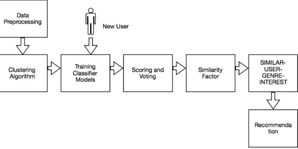
Figure 1: Pipeline for Proposed Solution
Fig. 1 gives an overall idea of the system pipeline design. We preprocess the data using WEKA [4]. After this, the attributes are given as an input to a clustering algorithm. We train classification models on the clustered data. These classifiers are
then used to assign new users to a cluster. Then, for the new user we analyze and calculate the similar users from within the assigned cluster. After this, we calculate the most frequent genres from the list of movies that the similar users have rated highly. Using this information, we recommend those movies with a high rating and top genre to the new users.
3.3 Data Preprocessing
The standard MovieLens dataset is used. Other than all the necessary movie attributes such as ratings, movie IDs and genre, we utilize user demographics associated with user IDs. Our goal at this stage is to transform the data into appropriate format which could be interpreted by the WEKA tool. Once in its native format, the tool analyzes the attributes and we can conduct experiments by subjecting the data to various preprocessing mechanisms, machine learning algorithms, classification techniques and generate metrics with statistical analysis. We perform preprocessing using the following steps:
1. Load file containing demographic information of users in WEKA GUI Explorer, one of the many suites available within the WEKA framework
2. Open the file using the ARFF editor
3. Remove the user ID information associated with the demographic attributes 4. Save the file as .arff
We now have our data in the required format.
3.4 Clustering Algorithm
The preprocessed data is now subjected to clustering. In clustering, data is meaningfully grouped in different sets, called clusters based on the demographic variety [4]. Clustering allows us to segregate data so that we can concentrate only
on a specific subset for obtaining relevant information. Since one of the objectives is to decrease the amount of data being processed, clustering serves as a simple, yet effective msachine learning technique to achieve the same. In our experiments we explore three different clustering mechanisms:
3.4.1 K-means
K-means is a partitioning based clustering algorithm, which is useful in separating data into ’k’ number of clusters which are independent of each other [14]. In big data, k-means is one of the simplest machine learning technique which allows researchers to investigate a subset of the entire dataset for experiments and analysis. In our use case, we segregate users based on their demographic attributes into ’k’ clusters. K-means can be implemented using the following steps [15]:
1. Initialize all the data points within the space. 2. Randomly select ’k’ cluster centers.
3. Calculate euclidean distance between each datapoint and cluster center. 4. If the distance of a datapoint to a specific cluster center is minimum as compared
to the other cluster centers, we assign the datapoint to former cluster. 5. Recompute new cluster center.
6. If re-assignment of a datapoint does not take place, then stop the algorithm, else repeat step (3).
This method ensures that the location of these datapoints will keep changing until the distance metric change is negligible. Also, k-means could run for a fixed number of iterations as a termination condition. For our experiments distance between cluster
center and datapoint is calculated using Euclidean distance, represented as [15]: 𝐸𝑢𝑐𝑙𝑖𝑑𝑒𝑎𝑛 𝐷𝑖𝑠𝑡𝑎𝑛𝑐𝑒 = ⎯ ⎸ ⎸ ⎷ 𝑛 ∑︁ 𝑖=1 (𝑦−𝑦𝑖)2 (1)
where yi = datapoint in consideration
y = centroid in consideration where yi ̸= y
n = total number of datapoints
3.4.2 Expectation Maximization
Expectation Maximization transforms the data into linear combinations of a variety of normal distributions where the aim is to continually find the maximum likelihood (log likelihood) until there is no change of this value within the data [15]. So there are two critical steps within EM: the expectation step and the maximization step. EM is implemented stepwise as follows:
1. In the expectation step, a function is derived which computes variable approxi-mation using log likelihood.
2. In the maximization step, this log likelihood function value is maximized which helps in computing the hidden variables within the next expectation step. 3. Stop the process when the log likelihood of the data does not change or is
negligible.
We choose expectation maximization as a technique to run our experiments with since it is resilient to noise in data, works well with linear data and there is no limit to the number of clusters which can be created.
3.4.3 Canopy Clustering
Canopy clustering is a sophisticated version of the k-means data clustering algorithm [16]. Like k-means, canopy clustering also relies on the distance metric for clustering data. The only difference is that canopy utilizes two thresholds (T1 and T2). Distance between a randomly chosen datapoint (canopy) and other points are calculated. If the distance is less than T1, that point is considered to be a strong point and gets assigned to the canopy. If the distance is less than even T2, then the point is considered to be weak and is removed from the set of points. This process is carried out iteratively with the remaining datapoints (which are not eliminated by the T2 threshold value). Canopy clustering can be implemented stepwise as follows:
1. Set the two thresholds T1 and T2 (T1 >T2).
2. Remove a datapoint from the collection of datapoints, this point is a new cluster(canopy).
3. For every remaining point in the set, assign to a new cluster (canopy) if the distance is less that T1.
4. If the distance is less that T2, we remove point from the set of points. 5. Repeat (2) until there are no more datapoints remaining.
This canopied data is then internally subject to the k-means clustering which gives us the final clustered data. In our experiments, we utilize this clustering technique for comparison between other techniques. All these algorithms are implemented using WEKA framework.
3.5 Training Classifier Models
The goal of clustering is to create meaningful subsets of data. It is essential to have a mechanism to process the data subset of interest without manually analyzing each
cluster. In order to tackle this problem as well as to improve the overall robustness of the system pipeline, we train the clustered data on various classifier models. This machine learning technique enables the system to access and analyze the cluster of interest with minimal possible computations involved. We train three classifier models on the clustered data:
3.5.1 Decision Stump
Decision stump is a weak one level classifier which is commonly used along with AdaBoost (Boosting) algorithms in order to improve the overall efficiency of the classifier [17]. Structurally, a decision stump tree consists of an internal node which is immediately connected to the terminal nodes. It practically bases its decision on a single attribute within the dataset. Decision stumps work on the principle of confidence rated predictions and work well in boosting techniques; where weak classifiers together form an overall strong classifier [18]. In paper [4], decision tree is used as a standalone classification model for cluster assignment.
3.5.2 J48
J48 classifier algorithm is a modification of the C4.5 algorithm [19]. The algorithm creates a decision tree based on a greedy top-down approach [20] where each attribute which can classify all instances in the best possible manner is considered. This process continues in a recursive fashion until all the data is classified. Normalized information gain, i.e. the difference of entropy levels found between attributes is utilized to select the best attribute for classification. The steps of the J48 algorithm are as follows:
1. Split each attribute of an instance until a subset of instances are present within the same class.
2. Leaves are labelled with the same class if instances are present within that class. 3. Information gain is calculated and the attribute with the highest entropy
differ-ence is used in making a decision.
4. A sublist created on the decision based on the best selected attribute is added as a child node to the decision node.
5. Repeat steps (1) to (4) on the sublist created.
J48 is a robust classification algorithm which works extremely well with continuous and distinct data which also allows for data pruning after the model is created. In paper [4], J48 is also used as a standalone classification model for cluster assignment.
3.5.3 Naive Bayes
Naive Bayes is a probabilistic approach to classifying large data sets. The underlying principle that the classification algorithm assumes is that the attributes are independent of each other [21]. Using the Bayes Theorem conditional probability, it calculates the instances which belong to a particular class.
3.6 Scoring and Voting
At this stage, the pre-requisites to the system are complete. We have different classifiers trained on the clustered data. So when a new user is exposed to the system, we need to ’’score’’ the user to assign him a cluster. The goal here is to discover a subset of the data which is significant to our new user in terms of further computations within the pipeline. As mentioned, we do not want to explore the entire dataset in order to achieve our final result. Scoring new user attributes against classifiers trained on the clustered data will decide the cluster of interest which makes the system efficient.
We use an ensemble technique in which all three trained classifiers predict the resultant cluster to which the new user should be associated. A majority vote decides the final cluster. Such a re-enforcement mechanism increases system robustness and ensures that the we do not assign an incorrect cluster.
3.7 Similarity Factor (SF)
The scoring and voting mechanism ensures that the incoming user is assigned to the appropriate cluster which allows us to find similar users, which is the next step in this proposed solution [4]. The goal here is to find as many similar users to the new user based on the given attributes. We find similar users in the following fashion:
Let (𝑢1, 𝑢2, 𝑢3...𝑢𝑖, ...𝑢𝑛) be the users in the cluster where target user v has been
classified (1≤𝑖≤𝑛)
Let sim(𝑢𝑖, v) be the similarity between user 𝑢𝑖 and v, then we have
𝑠𝑖𝑚(𝑢𝑖, 𝑣) = 𝑊𝑎𝑔𝑒𝑖+𝑊𝑔𝑒𝑛𝑑𝑒𝑟𝑖 +𝑊𝑜𝑐𝑐𝑢𝑝𝑎𝑡𝑖𝑜𝑛𝑖 (2)
Let,
v.age be the age of the target user 𝑢𝑖.age be the user 𝑢𝑖’s age
ageDifference = (max(age) - min(age) within cluster) then,
if(|𝑢𝑖.age - v.age|) < ageDifference
𝑊𝑎𝑔𝑒𝑖 = 1− |𝑢𝑖.𝑎𝑔𝑒−𝑣.𝑎𝑔𝑒| 𝑎𝑔𝑒𝐷𝑖𝑓 𝑓 𝑒𝑟𝑒𝑛𝑐𝑒 (3) else 𝑊𝑎𝑔𝑒𝑖 = 0 (4) if (𝑊𝑎𝑔𝑒𝑖 <0) 𝑊𝑎𝑔𝑒𝑖 = 0 (5) Let,
v.gender be the gender of the target user 𝑢𝑖.gender be the user 𝑢𝑖’s gender
then,
if(𝑢𝑖.gender == v.gender)
𝑊𝑔𝑒𝑛𝑑𝑒𝑟𝑖 = 1 (6)
else
𝑊𝑔𝑒𝑛𝑑𝑒𝑟𝑖 = 0 (7)
Let,
v.occupation be the occupation of the target user 𝑢𝑖.occupation be the user𝑢𝑖’s occupation
then,
if(𝑢𝑖.occupation == v.occupation)
𝑊𝑜𝑐𝑐𝑢𝑝𝑎𝑡𝑖𝑜𝑛𝑖 = 1 (8)
else
𝑊𝑜𝑐𝑐𝑢𝑝𝑎𝑡𝑖𝑜𝑛𝑖 = 0 (9)
In this way, the similarity factor of every old user within the cluster is calculated w.r.t the new user. Higher the similarity factor value, the more similar are the users. For the sake of our experiments we set the similarity factor threshold as 0.90, all users equal or above this value are considered to be similar. The intuition is that at least one attribute between the user and target user should the same. For example, if one of the attributes between gender, age and occupation of user and target user is the same, the similarity is at least 1. But in a situation where gender and occupation are not the same, but the target user’s age is within close range of the other, then according to equation (3), there is a possibility of getting a similarity value less than 1. Considering that the difference between user age and target user age is less, we set 0.90 as the similarity threshold.
3.8 SIMILAR-USER-GENRE-INTEREST
The goal is to provide a streamlined recommendation. To ensure this, we need to extract some meaningful information from the similar users based on demographics. The intutive idea is to calculate the most frequently rated genres and streamline rec-ommendations. We do this by choosing the movies rated highly by similar users which have genres matching the frequently rated genres. Calculated collective genres along with a high movie rating could serve as ideal parameters for movie recommendations at this stage.
For every new user, v, we can generate a genre of interest based on v’s similar users
1. For each of v’s similar user:
a. Create a hash map of genre-count
b. Find list of movies that the user has highly rated c. for each movie in list:
for each genre of the movie:
increment count of the genre in hash map of genre-count d. return top n-genres as those with the most counts
3.9 Recommendation
Using the SIMILAR-USER-GENRE-INTEREST information, we flag only those movies which belong to the pool of genres and whose movie rating is high. All flagged movies are then brought up as recommendations to the new user within the system.
3.10 Steps In The Proposed Pipeline
We summarize the steps involved in our proposed pipeline as follows: 1. Format user data file to user.arff.
2. To cluster users in ’k’ clusters:
a. Obtain clusters using either k-means, EM or canopy clustering algorithms. b. Save this file as ucluster.arff.
3. Train Decision Stump, J48 and Naive Bayes classifier models with ucluster.arff as input.
4. For each new user v: a. For each classifier:
i. Obtain prediction score for each cluster.
ii. Consider classifier vote as the cluster with the highest prediction score.
b. Use voting to assign final cluster to user:
i. Assign the cluster voted by majority of classifiers.
ii. In case of no majority vote, assign cluster with the highest prediction score.
c. Generate similar users for v: Compute similarity factor between v and users within the cluster.
d. Compute SIMILAR-USER-GENRE-INTEREST .
e. Recommend movies to v, based on the top 4 genres selected by SIMILAR-USER-GENRE-INTEREST.
We implement the cluster generation and classification models by utilizing WEKA framework JAR files on the classpath of a shell file (.sh) which houses the actual cluster generation/classification model commands. The voting and scoring phase is
executed in a similar manner using a shell script pointing to the WEKA JAR files. SF and SIMILAR-USER-GENRE-INTEREST computations are implemented using Java code.
CHAPTER 4
Experimental Results and Analysis
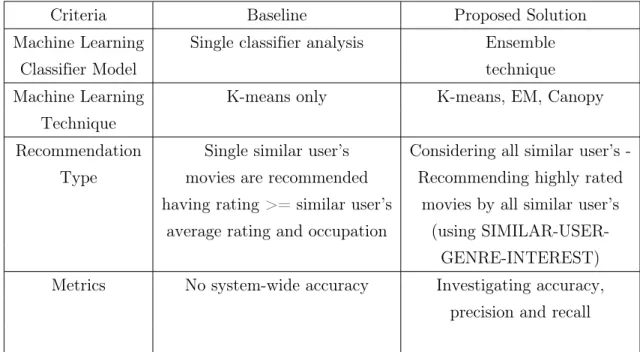
We establish paper [4] as our baseline paper. In Table 1 we see the difference between the proposed solution and the baseline.
Table 1: Differences between Proposed Solution and Baseline Criteria Baseline Proposed Solution Machine Learning Single classifier analysis Ensemble
Classifier Model technique
Machine Learning K-means only K-means, EM, Canopy Technique
Recommendation Single similar user’s Considering all similar user’s -Type movies are recommended Recommending highly rated
having rating >= similar user’s movies by all similar user’s average rating and occupation (using
SIMILAR-USER-GENRE-INTEREST) Metrics No system-wide accuracy Investigating accuracy,
precision and recall
4.1 Parameter Selection for Process Pipeline
4.1.1 Choosing the Number of Clusters (NoC)
All our experiments were implemented using 3 clusters.
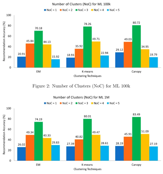
Fig. 2 and Fig. 3 refers to the system accuracy vs the number of clusters for the EM, K-means and Canopy clustering algorithms in MovieLens 100k and 1M datasets respectively. The accuracy increases from NoC = 1 to NoC = 3. This is because the false positive rates are high for NoC = 1 and NoC = 2. We get the highest system accuracy for all algorithms when we set NoC = 3. Increasing the number of clusters more than 3 also causes a decrease in the accuracy of the recommendation.
Figure 2: Number of Clusters (NoC) for ML 100k
Figure 3: Number of Clusters (NoC) for ML 1M
4.1.2 Choosing the Number of Genres (NoG) for Recommendation
Fig. 4 and Fig. 5 refer to system accuracy vs number of genres for EM, K-means and Canopy clustering algorithms in the MovieLens 100k and 1M dataset respectively. System accuracy increases as we increase NoG = 1 to NoG = 4. Increasing the NoG greater than 4 decreases the overall system accuracy. Examining the data dump
we see an increase in false positives as we keep increasing the number of genres for recommendation.
That is why we choose NoG = 4 for our experiments.
Figure 4: Number of Genres (NoG) for ML 100k
4.2 Classification Accuracy
We utilize the WEKA frameworks functionality to generate our classification models. They are created using a 10-fold stratified cross-validation mechanism. We create these classifiers keeping the number of clusters as 3.
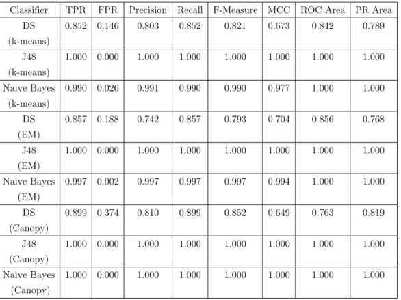
Table 2 and Table 3 show metrics generated by the WEKA framework for the 100k and 1M dataset respectively. We see the TPR, FPR, Precision, Recall, F-Measure, Matthews Correlation Coefficient (MCC), ROC curve area and PR curve area. These characteristics help us develop a deeper understanding about the overall robustness of the classification strategies used per machine learning technique. It can be seen that the J48 classification algorithms perform outstandingly well in both the data sets as per the metrics. Decision stump on the other hand performs poorly in terms of the metrics for the k-means clustering algorithm in the 1M dataset and its overall performance as per the metrics is less compared to the other classifier models.
From Fig. 6 - Fig. 7, we observe that J48 and Naive Bayes classifier models classify data instances correctly with a very low misclassification rate. The decision stump on the other hand has a huge misclassification rate in both the 100k and 1M datasets for all the machine learning algorithms (this is further elaborated on in the next section). The decision stump classification results are better for EM and canopy clustering in comparison to k-means, which is why we are considering its decision in conjuction with the votes given by other classifiers, but is not a practical solution on its own.
4.3 Decision Stump Analysis
From Table 2 and Table 3, we see that decision stump classifier model has low values for different metrics. The number of misclassfied instances are more for all the
Table 2: WEKA metrics for K-means, EM and Canopy (100k)
Classifier TPR FPR Precision Recall F-Measure MCC ROC Area PR Area
DS 0.852 0.146 0.803 0.852 0.821 0.673 0.842 0.789 (k-means) J48 1.000 0.000 1.000 1.000 1.000 1.000 1.000 1.000 (k-means) Naive Bayes 0.990 0.026 0.991 0.990 0.990 0.977 1.000 1.000 (k-means) DS 0.857 0.188 0.742 0.857 0.793 0.704 0.856 0.768 (EM) J48 1.000 0.000 1.000 1.000 1.000 1.000 1.000 1.000 (EM) Naive Bayes 0.997 0.002 0.997 0.997 0.997 0.994 1.000 1.000 (EM) DS 0.899 0.374 0.810 0.899 0.852 0.649 0.763 0.819 (Canopy) J48 1.000 0.000 1.000 1.000 1.000 1.000 1.000 1.000 (Canopy) Naive Bayes 1.000 0.000 1.000 1.000 1.000 1.000 1.000 1.000 (Canopy)
Figure 6: Classifier Model Accuracy for ML 100k machine learning algorithms in both the 100k and 1M data sets.
Table 3: WEKA metrics for K-means, EM and Canopy (1M)
Classifier TPR FPR Precision Recall F-Measure MCC ROC Area PR Area
DS 0.691 0.164 0.519 0.691 0.590 0.512 0.812 0.616 (k-means) J48 1.000 0.000 1.000 1.000 1.000 1.000 1.000 1.000 (k-means) Naive Bayes 0.973 0.011 0.975 0.973 0.973 0.963 0.997 0.994 (k-means) DS 0.963 0.041 0.929 0.963 0.945 0.925 0.969 0.931 (EM) J48 1.000 0.000 1.000 1.000 1.000 1.000 1.000 1.000 (EM) Naive Bayes 0.998 0.003 0.998 0.998 0.998 0.995 1.000 1.000 (EM) DS 0.834 0.134 0.740 0.834 0.782 0.701 0.845 0.728 (Canopy) J48 1.000 0.000 1.000 1.000 1.000 1.000 1.000 1.000 (Canopy) Naive Bayes 0.999 0.001 0.999 0.999 0.999 0.998 1.000 1.000 (Canopy)
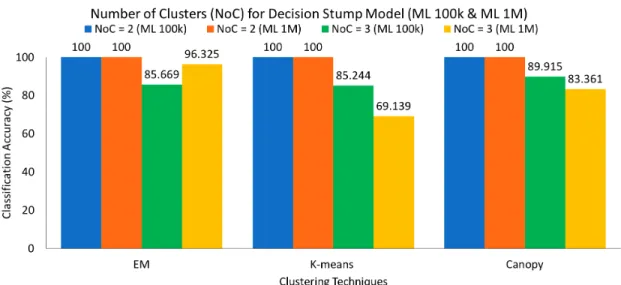
where we run decision stump classifier where the number of clusters are set to 2 & 3 respectively for all the machine learning algorithms. It can be seen from Fig. 8 that there is a huge decrease in classification accuracy when the cluster size is increased to 3. We know that the decision stump is a one-level decision tree which on its own is a very weak classifier. On observing the dataset, we have the following attributes:
Table 4: Attributes of data instances user ID gender age occupation
The decision stump algorithm needs only a single attribute to make a classification decision. By default, it chooses the attribute with exactly two values. On scanning the datapoints it recognizes gender to be an attribute which can take two values either ’male’ or ’female’. So it makes a decision based on this attribute. When we set the number of clusters to 3, it is unable to make a decision based on the gender attribute alone since there are 3 clusters in which to classify the instances. This causes a huge misclassification and low accuracy in terms of correctly classified instances. In another experiment, we ran the algorithm on the dataset without the gender attribute, the algorithm then changes its classification criterion to the age attribute where it computes the average age of all datapoints. Datapoints with age more than the average is put in one cluster and those with age less than average in another. In this way, it is able to classify into two clusters [18].
Thus we use an ensemble technique which acts as a re-enforcing mechanism and ensures that we assign the appropriate cluster to the new user.
4.4 System Accuracy
The baseline paper does not provide a system wide (recommendation) accuracy for its proposed solution. So in order to establish a baseline accuracy metric, we calculate the accuracy of the baseline which is 46.335% for the MovieLens 100k and
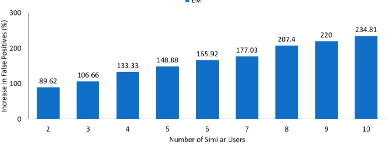
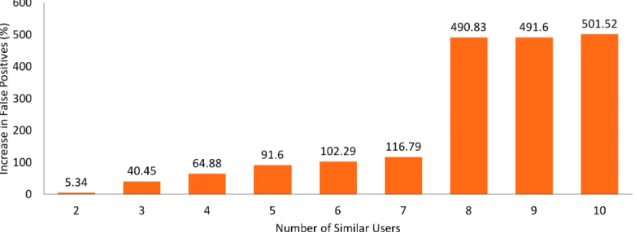
Figure 8: Number of Clusters (NoC) for Decision Stump Model (ML 100k & ML 1M) 51.77% for the 1M dataset. We observed the movie recommendation data dump for this approach and noticed that the number of false positives contributed towards the low accuracy measure. In Fig. 9 - Fig. 14 we increased the number of similar users whose movies were being recommended to the new user and observed an increase in percentage of false positives w.r.t a single similar user (in the baseline) for all clustering techniques and datasets. The understanding here is that, the baseline computes similar users and then recommends movie list from the best similar user having a rating which is greater than or equal to their calculated average rating and occupation. On observing the dump, we see that there were many movies which were falsely classified as recommendations. This fact shows promise for using the SIMILAR-USER-GENRE-INTEREST algorithm.
To improve the accuracy of the overall system, we rely on providing relevant, personalized recommendations by using the genre attribute. We chose 15 users randomly as part of our test set. We filter the recommendations based on the user genre. After calculating similar users, we compute
SIMILAR-USER-GENRE-Figure 9: Percentage Increase in False Positives (compared to 1 similar user) on Increasing Number of Similar Users in Baseline for ML 100k using EM clustering
Figure 10: Percentage Increase in False Positives (compared to 1 similar user) on Increasing Number of Similar Users in Baseline for ML 1M using EM clustering INTEREST of all the similar users. By doing so, we filter and stream line the recommendation to new user. We get the best results with the canopy clustering algorithm with an accuracy of 83.49% as seen in Fig. 16. There is an increase in accuracy as the size of the dataset increases. Precision and Recall rates for the 100k
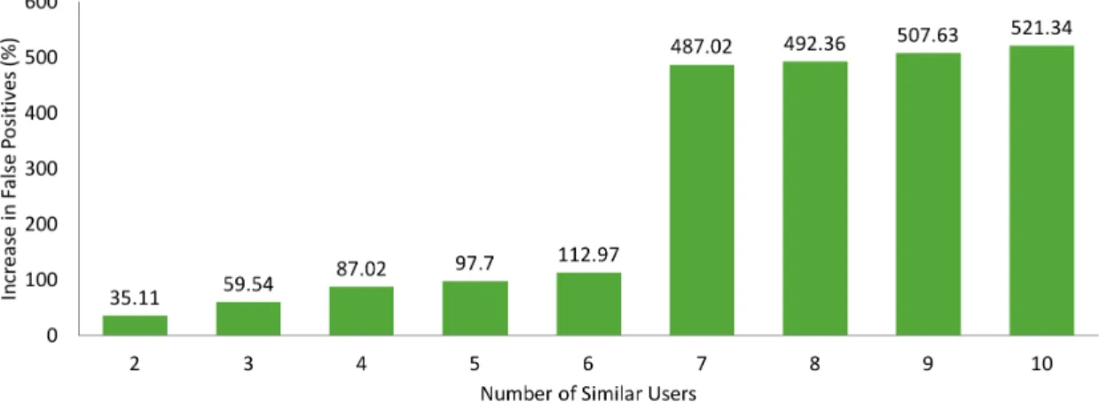
Figure 11: Percentage Increase in False Positives (compared to 1 similar user) on Increasing Number of Similar Users in Baseline for ML 100k using K-means clustering
Figure 12: Percentage Increase in False Positives (compared to 1 similar user) on Increasing Number of Similar Users in Baseline for ML 1M using K-means clustering dataset fluctuates as seen in Fig. 15, whereas for the 1M dataset it is almost consistent (3% - 4 % change).
For clarity we define the metrics we use to determine robustness of our proposed solution:
Figure 13: Percentage Increase in False Positives (compared to 1 similar user) on Increasing Number of Similar Users in Baseline for ML 100k using Canopy clustering
Figure 14: Percentage Increase in False Positives (compared to 1 similar user) on Increasing Number of Similar Users in Baseline for ML 1M using Canopy clustering
𝐴𝑐𝑐𝑢𝑟𝑎𝑐𝑦 = 𝑇 𝑃 +𝑇 𝑁
𝑇 𝑃 +𝑇 𝑁+𝐹 𝑃 +𝐹 𝑁 (10)
𝑃 𝑟𝑒𝑐𝑖𝑠𝑖𝑜𝑛= 𝑇 𝑃
𝑅𝑒𝑐𝑎𝑙𝑙= 𝑇 𝑃
𝑇 𝑃 +𝐹 𝑁 (12)
Figure 15: Overall Recommendation Accuracy, Precision and Recall for ML 100k
Figure 16: Overall Recommendation Accuracy, Precision and Recall for ML 1M
4.5 Runtime Analysis
The statistics in Table 5 and Table 6 show when a single user is exposed to the pipeline. We represent the analysis graphically in Fig. 17 and Fig. 18 respectively. We
measured system performance time for the baseline and our proposed approach to see if there is a difference in runtime for both methods. As expected, we see a significant increase in computation time for the larger 1M and 100k dataset as compared to the baseline. This increase in runtime for the proposed solution is due to the post processing involved in SIMILAR-USER-GENRE-INTEREST computation and then recommending movies as opposed to the simple look-up of similar user movies.
Table 5: Runtime analysis (ML 100k, 943 users)
ML Training Post Total Percentage
Technique And Scoring (ms) Procesing (ms) Time (ms) Increase In Runtime
Baseline 1250 836 2086 N/A
EM 1140 1974 3114 49.28%
K-means 1250 1839 3089 48.08%
Canopy 1190 2163 3353 60.73%
Table 6: Runtime analysis (ML 1M, 6040 users)
ML Training Post Total Percentage
Technique And Scoring (ms) Procesing (ms) Time (ms) Increase In Runtime
Baseline 1540 5710 7250 N/A
EM 1420 10338 11758 62.17%
K-means 1540 9812 11352 56.57%
Canopy 1540 11369 12909 78.05%
CHAPTER 5 Conclusion
The proposed method is promising in terms of generating recommendations for new users with no prior history in the system. The use of ensemble classification models in categorizing new users is efficient and reliable as seen by its high classification accuracy and re-enforcing mechanism after which potential similar users are filtered out using the similarity factor metric. This method alleviates one of the drawbacks of collaborative filtering which suffers from cold start. There is a possibility of generalizing the proposed method which can further be applied to any recommender system, as long as user demographics and system-specific item characteristics are available.
CHAPTER 6 Future Work
Recommender systems are usually of two types: relevant recommendations and diverse recommendations. Using only user demographics can work so much as to provide an entry point to the new user within the system. The proposed system aims at a focused, streamlined recommendation, a recommender system of the former type. Diverse recommendations are important in any product platform since it broadens user perspective, which essentially translates to more data which could be leveraged to improve recommendation quality, system performance etc. The variety in accurate recommendations could increase user base and revenue stream for the platform. An example of diverse recommendations within this scenario could be combining demographic and social media information of a user, to get a varied recommendation. With this idea in mind, research could be conducted to provide for diverse recommendations as well in a cold start scenario.
This paper concentrates only on the new user recommendation problem. The use of demographics in conjunction with product information could also be used to explore new product or new user to new product problems of cold start as well. For example, develop some heuristics between people of specific demographics who buy/own/rate certain products. Such a model could be used to analyze the latter two problems of cold start.
A caching mechanism for the proposed solution where recommendation lists for new users are stored, so we do not need to recompute similarity and collective genre information which should ideally reduce the runtime. The recommendation list can be updated after a specified time frame in order to incorporate latest movie related information.
LIST OF REFERENCES
[1] P. Parhi, A. Pal, and M. Aggarwal, ‘‘A survey of methods of collaborative filtering techniques,’’ pp. 1--7, 2017.
[2] M. Agrawal, T. Gonçalves, and P. Quaresma, ‘‘A hybrid approach for cold start recommendations,’’ pp. 1--6, 2017.
[3] A. Sang and S. K. Vishwakarma, ‘‘A ranking based recommender system for cold start data sparsity problem,’’ pp. 1--3, 2017.
[4] A. K. Pandey and D. S. Rajpoot, ‘‘Resolving cold start problem in recommendation system using demographic approach,’’ pp. 213--218, 2016.
[5] J. Bobadilla, F. Ortega, A. Hernando, and A. GutiéRrez, ‘‘Recommender systems survey,’’ Know.-Based Syst., vol. 46, pp. 109--132, July 2013.
[6] P. Melville and V. Sindhwani, ‘‘Recommender systems,’’ pp. 829--838, 2010. [7] X. Su and T. M. Khoshgoftaar, ‘‘A survey of collaborative filtering techniques,’’
Adv. in Artif. Intell., vol. 2009, pp. 4:2--4:2, Jan. 2009.
[8] S. Solanki and D. S. Batra., ‘‘Recommender system using collaborative filtering and demographic characteristics of users,’’ International Journal on Recent and
Innovation Trends in Computing and Communication (IJRITCC), vol. 3, pp.
4735 -- 4741, July 2015.
[9] X. Li, ‘‘Collaborative filtering recommendation algorithm based on cluster,’’ vol. 4, pp. 2682--2685, 2011.
[10] P. Nair, M. Moh, and T. S. Moh, ‘‘Using social media presence for alleviating cold start problems in privacy protection,’’ pp. 11--17, 2016.
[11] A. Bhatia, ‘‘Community detection for cold start problem in personalization: Com-munity detection is large social network graphs based on users 2019; structural similarities and their attribute similarities,’’ pp. 167--171, 2016.
[12] C. A. Q. Rana, H. Salima, F. Usama, and C. Hammam, ‘‘From a "cold" to a "warm" start in recommender systems,’’ pp. 290--292, 2014.
[13] J. J. Vie, F. Yger, R. Lahfa, B. Clement, K. Cocchi, T. Chalumeau, and H. Kashima, ‘‘Using posters to recommend anime and mangas in a cold-start scenario,’’ vol. 03, pp. 21--26, 2017.
[14] S. Arora and I. Chana, ‘‘A survey of clustering techniques for big data analysis,’’ pp. 59--65, 2014.
[15] G. Ahalya and H. M. Pandey, ‘‘Data clustering approaches survey and analysis,’’ pp. 532--537, 2015.
[16] H. Zhou, X. Ma, L. Zhou, Z. Yu, and X. Zeng, ‘‘An efficient parallel method for canopy clusteing with multi-core platform,’’ pp. 1--3, 2014.
[17] D. Su, P. Fung, and N. Auguin, ‘‘Multimodal music emotion classification using adaboost with decision stumps,’’ pp. 3447--3451, 2013.
[18] X. Jun, Y. Lu, Z. Lei, and X. Hui, ‘‘Boosting decision stumps to do pairwise classification,’’ Electronics Letters, vol. 50, no. 12, pp. 866--868, 2014.
[19] N. Bhargava, S. Sharma, R. Purohit, and P. S. Rathore, ‘‘Prediction of recurrence cancer using j48 algorithm,’’ pp. 386--390, 2017.
[20] N. Satyanarayana, Y. Ramadevi, and K. K. Chari, ‘‘High blood pressure prediction based on AAA using J48 classifier,’’ pp. 121--126, 2018.
[21] N. Kumar and S. Khatri, ‘‘Implementing weka for medical data classification and early disease prediction,’’ pp. 1--6, 2017.