Incremental and Parallel
Learning Algorithms for Data
Stream Knowledge Discovery
Doctoral Thesis
byLei Zhu
Submitted in Partial Fulfillment of the Requirements of the
D.Comp. Program
Department of Computing and Information Technology UNITEC Institute of Technology
New Zealand Feb 2018
Incremental and parallel are two capabilities for machine learning algorithms to accommodate data from real world applications. Incre-mental learning addresses streaming data by constructing a learning model that is updated continuously in response to newly arrived sam-ples. To solve the computational problems posed by large data sets, parallel learning distributes the computational efforts among multiple nodes within a cloud or cluster to speed up the calculation. With the rise of BigData, data become simultaneously large scale and stream-ing, which is the motivation to address incremental and parallel incre-mental (PI) learning in this work.
This research first considers the incremental learning alone, in the graph max-flow/mcut problem. An augmenting path based in-cremental max-flow algorithm is proposed. The proposed algorithm handles graph changes in a chunking manner, updating residual graph via augmentation and de-augmentation in response to edge capacity increase, decrease, edge/node adding and removal. The theoretical guarantee of our algorithm is that incremental max-flow is always equal to batch retraining. Experiments show the deterministic com-putational cost save (i.e., gain) of our algorithm with respect to batch retraining in handling graph edge adding.
The proposed incremental max-flow is then applied to upgrade an existing batch semi-supervised learning algorithm known as graph minicuts to be incremental. In batch graph minicuts, a graph is learned from input labeled and unlabeled data, and then a min-cut is con-ducted on that graph to make the classification decision. In the pro-posed modification, the graph is updated dynamically for accommo-dating online data adding and retiring. Then the proposed incremen-tal max-flow algorithm is adopted to learn min-cut from the resulting
that the proposed algorithm outperforms state-of-the-art stream clas-sification algorithms.
In the incremental max-flow, the training speed is not satisfactory when the data set is huge. A straightforward solution is to combine parallel data processing with incremental learning. Previously, par-allel and incremental learning are often treated as two separate prob-lems and solved one after another. Alternatively in this work, these two learning problems are solved in one process (i.e., PI integration).
To simplify the learning, this research considers a base model in which incremental learning can be implemented by merging knowl-edge from incoming data and parallel learning can be performed by merging knowledge from simultaneous learners (i.e., in knowledge mergeable condition). As a result, this work develops a parallel in-cremental wESVM (weighted Extreme Support Vector Machine) algo-rithm, in which the parallel incremental learning of the base model is completed within a single process of knowledge merging. Specifi-cally, the wESVM is reformulated such that knowledge from subsets of training data can be merged via simple matrix addition. As such, the proposed algorithm is able to conduct parallel incremental learn-ing by merglearn-ing knowledge from data slices arrivlearn-ing at each incremen-tal stage. Both theoretical and experimenincremen-tal studies show the equiva-lence of the proposed algorithm to batch wESVM in terms of learning effectiveness. In particular, the algorithm demonstrates desired scala-bility and clear speed advantages to batch retraining.
In the field of data stream knowledge discovery, this work investi-gates incremental machine learning and invents a wESVM-based par-allel learning and incremental learning integrated system. The limi-tation of this work is that PI integration applies only to models that satisfy the knowledge mergeable condition. Future work should in-vestigate how to release this constraint and expand PI integration to other models such as SVM and neural network.
First and foremost I want to thank my supervisors Prof. Shaoning Pang, Prof. Abdolhossein Sarrafzadeh and Prof. Kazushi Ikeda. It has been an honor to be their doctorate student. I really appreciate all their contributions of suggestions, time, and guidance to make my doctorate experience productive and stimulating. The passion they have for their research is motivational and contagious for me. I am also thankful for very useful and essential comments they have pro-vided, helping to keep me on the right track.
I would like to thank Dr. Chandimal Jayawardena and Dr. Iman Ardekani for their help throughout the D.Comp. Program. I am also grateful to Prof. Dennis Viehland for his great contribution on helping improve the language of this thesis.
Finally, I would like to thank all members of the DMLI group, which has been a source of friendships as well as useful suggestions and collaboration. This includes, but is not limited to: Lei Song, Jane Zhao, Yiming Peng, Simon Dacey, Peter Zhang, Shahid Ali, Denis Lavrov, Tony Shi, Steven Zhang, Holmes He, Fred Li, Veronique Blanchet, David Lu, Elle Musoke, and Charles Duan.
Abstract iii Acknowledgements v 1 Introduction 2 1.1 Background . . . 2 1.2 Research Roadmap . . . 3 1.3 Contribution . . . 5 1.4 Thesis Organization . . . 7
2 Max-flow Problem and Max-flow Algorithms 9 2.1 Introduction . . . 9
2.1.1 Definitions and Problem Statement . . . 9
2.1.2 Max-flow Applications . . . 11
2.2 Batch Max-flow Algorithms . . . 14
2.2.1 Augmenting Path . . . 14
2.2.2 Boykov-Kolmogorov (BK) Algorithm . . . 15
2.2.3 Incremental Breadth First Search (IBFS) Algorithm 19 2.2.4 Push Relabel Algorithm . . . 23
2.3 Incremental Max-flow Algorithms . . . 28 vii
2.3.1 Incremental Push Relabel . . . 28
2.3.2 Excesses IBFS Algorithm . . . 34
2.4 Summary . . . 38
3 Proposed Incremental Max-flow Algorithm 40 3.1 Introduction . . . 40
3.1.1 Motivation . . . 40
3.2 Preliminary . . . 42
3.3 Proposed Incremental and Decremental Max-flow Al-gorithm . . . 44
3.3.1 Incremental Max-Flow Setup . . . 44
3.3.2 Decremental Max-Flow . . . 46
3.3.3 Incremental Max-flow . . . 52
3.3.4 Complexity Analysis . . . 54
3.4 Experiments and Discussions . . . 55
3.4.1 Experiment Setup . . . 55
3.4.2 Results of Learning Graphs Continuously Expand-ing . . . 56
3.4.3 Results of Learning Graphs Continuously Shrink-ing . . . 58
3.5 Summary . . . 61
4 Implement the Proposed Incremental Max-flow on Semi-supervised Learning 66 4.1 Introduction . . . 66
4.1.1 Semi-supervised Learning . . . 66
4.1.2 Graph Mincuts Algorithm . . . 67
4.2 Preliminary . . . 69
4.2.1 Graph Construction . . . 69
4.2.2 Solve Min-Cut . . . 70
4.3 Implement Incremental Decremental Max-flow on In-cremental Semi-supervised Learning . . . 71
4.3.1 Graph Updating . . . 72 viii
4.3.2 Min-cut Updating . . . 72
4.4 Experiments and Discussions . . . 73
4.4.1 Graphical Demonstration . . . 73
4.4.2 Static Classification . . . 78
4.4.3 Drifting Concept Tracing . . . 80
4.4.4 Stream Learning . . . 82
4.5 Summary . . . 85
5 Parallel Incremental Learning Integration 89 5.1 Introduction . . . 89
5.2 Motivation: PI Integration via Knowledge Merging . . 90
5.3 Knowledge Mergeable Algorithms . . . 91
5.3.1 LPSVM . . . 91
5.3.2 ESVM . . . 94
5.3.3 wLPSVM and wESVM . . . 95
5.4 Summary . . . 98
6 Proposed PI integrated algorithm 100 6.1 Introduction . . . 100
6.2 Preliminary . . . 101
6.3 Proposed PI Integrated wESVM . . . 102
6.3.1 wESVM Reformulation for Merging . . . 103
6.3.2 Incremental and Decremental wESVM . . . 108
6.3.3 PI Integrated wESVM . . . 110
6.3.4 MapReduce based Implementation . . . 114
6.3.5 Speedup Analysis . . . 117
6.4 Experiments . . . 120
6.4.1 Equivalence to Batch Retraining . . . 121
6.4.2 Parallel Efficiency Evaluation . . . 121
6.4.3 Incremental Effectiveness . . . 126
6.4.4 Comparison with Other Algorithms . . . 128
6.5 Summary . . . 130 ix
7 Conclusion and Future Works 135
7.1 Conclusion . . . 135 7.2 Future Works . . . 137
1.1 The research roadmap of this thesis. . . 6 2.1 An example of graphs min-cut used for computer
vi-sion applications. Left is the graph constructed and the right is the min-cut result. . . 11 2.2 An example of max-flow search through augmenting
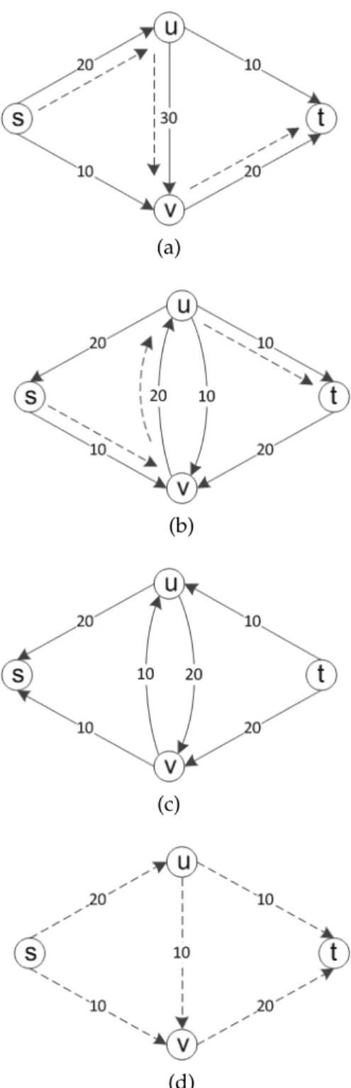
path. (a) initial residual graph with the first found s− t path shown in dotted lines; (b) augmented residual graph with newly found s − t path; (c) current aug-mented residual graph, where augmenting path termi-nates since no more s − t path can be found; (d) the obtained actual max-flow. . . 16 2.3 An example of trees S and T in BK algorithm.
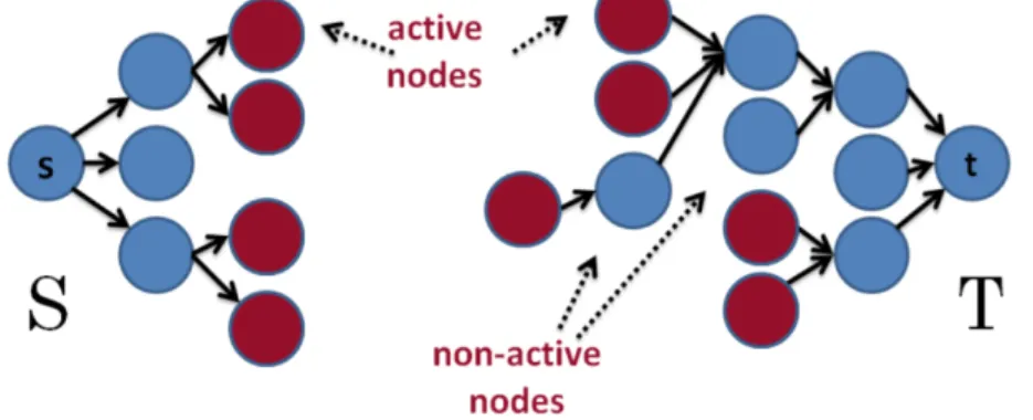
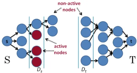
Non-active and Non-active nodes are marked as blue and red re-spectively. . . 17
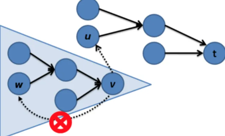
2.4 An example of the search trees S (red nodes) and T (blue nodes) at the end of the growth stage when a path (yellow line) from the source s to the sink t is found. Active and passive nodes are labeled by letters A and P, correspondingly. Free nodes appear in black. . . 17 2.5 An example of adoption step on a nodev. An orphan
sub-tree is shown in the triangle. The solid edges are residual edges which are tree edges and the dashed edges are residual edges which are not tree edges. Nodeucan be selected as a parent ofv. Butwcannot be selected as a parent forv, because there is no residual path fromw tot(the path terminates atv). . . 18 2.6 An example of a forward pass of IBFS. Note that during
a forwardSgrown pass, active nodes exist only in level DsofS. . . 20
2.7 An example of augmentation step of IBFS. The parent edges of the orphan nodes are saturated during this augmentation. The triangles represent the orphan sub trees that are created after the augmentation. Note the augmenting path is always a shortest s−t path in the residual graph. . . 21 2.8 An example of adoption step of IBFS, in which orphan
vis relabeled. The solid edges are residual edges which are tree edges. The dashed edges are residual edges which are not tree edges. The triangles represent or-phan sub trees. Node v finds uas the lowest potential parent and performs a relabel withuas his new parent. The children ofv then become orphans themselves and will be processed later during this adoption phase. . . 22 2.9 An example of max-flow search through push relabel.
Part A . . . 26 xii
2.10 An example of max-flow search through push relabel. Part B . . . 27 3.1 An example of cycle flow. (a) the residual graph; (b) the
actual flow. . . 47 3.2 An example of the formation of a cycle flow in flow
changing. (a) the initial s − t flow s − a− b − c−t; (b) a news−tflows−c−a−tis added due to newly inserted edges; (c) flows−a−tremoved due to edge removal; (d) flows−c−tremoved due to edge removal, what left is a cycle flowa−b−c−a. . . 62 3.3 An example of cycle flow cancellation. (a) initial graph;
(b) initial residual graph; (c) initial flow; (d) objective graph, where edge(u, v)need to be removed from ini-tial graph; (e) a u−v path is found in current residual graph; (f) the complete cycle u −w −v −u is found; (g) the residual graph after sending1 flow along cycle u−w−v−u; (h) now edge(u, v)can be removed safely. 63 3.4 An example of decremental max-flow learning through
de-augmentation. (a) objective graph; (b) initial resid-ual graph, a flow of 10 should be sent from v to u in order to release the capacity on (u, v); (c) a t −s path goes through(v, u)shown in dotted lines; (d) residual graph after de-augmenting thet−spath, now(u, v)has enough capacity to be reduced; (e) reduce the capacity of(u, v)by30and remove the empty edge, and obtain the residual graph of (a); (f) the actual max-flow on (a). 64 3.5 Gain and ANr for graph expanding . . . 65 3.6 Gain and ANr for graph shrinking . . . 65 4.1 Graphical demonstration of the proposed algorithm. Part
A . . . 74 xiii
4.2 Graphical demonstration of the proposed algorithm. Part B . . . 76 4.3 Graphical demonstration of the proposed algorithm. Part
C . . . 77 4.4 oMincut incremental and decremental learning on five
stages concept drift, with the final stage compared to batch learning. The transductive performance in terms of classification error rate is given at each stage in paren-theses as (a) (6.43 percent), (b) (3.59 percent), (c) (4.46 percent), (d) (3.20 percent), (e) (4.40 percent) and (f) (4.40 percent). . . 83 4.5 Two stream learning scenarios . . . 84 4.6 Sliding window snapshot learning on KDD streams . . 86 4.7 The variation of learners performance against the label
ratio. . . 87 4.8 The variation of learners performance against the label
ratio. . . 87 6.1 MapRedce work flow . . . 101 6.2 Running time against data size . . . 123 6.3 Speedup in terms of total execution time and node
av-erage time . . . 124 6.4 Speedup at Map and Reduce phases . . . 125 6.5 Percentage of time taken by Map and Reduce at
differ-ent data sizes . . . 127 6.6 Training time comparison . . . 133
3.1 Notations . . . 41
3.2 Results for graph expanding on 500 nodes . . . 57
3.3 Results for graph shrinking on 500 nodes . . . 59
3.4 Results for graph shrinking on 50 nodes . . . 60
4.1 Notations . . . 68
4.2 Accuracy comparison on UCI datasets . . . 79
4.3 Two-class recall comparison on imbalanced datasets . . 81
6.1 Incremental (Inc), parallel (Par) and PI integrated (PI) wESVM learning outcome differences against that of batch wESVM. . . 121
6.2 Training time of batch, incremental (Inc), Parallel (Par) and PI integrated (PI) wESVM algorithm . . . 128
6.3 Datasets description . . . 129 6.4 Classification capability without class-imbalance. Exp. 1 131 6.5 Classification capability with class-imbalance. Exp. 2 . 132
Chapter 1
Introduction
1.1
Background
The goal of machine learning can be stated as to build a computational model from what has been observed in the past Gama (2012). In the early days, research studies and practices in machine learning focused on batch learning, in which the complete data set is available at once to the algorithm that generates a decision model. The assumption be-hind batch learning is that samples are generated randomly according to a stationary probability distribution. The learning objective is to es-timate this distribution with the samples that are available.
Fast developments in information and communication technolo-gies, data collection and processing methods have introduced dra-matic changes. Currently, data are often presented in continuous streams, representing the current state of a stationary or non-stationary envi-ronment Muthukrishnan et al. (2005). To learn from these data streams, incremental learning constructs a learning model that is updated con-tinuously in response to newly arrived samples Joshi & Kulkarni (2012).
For the incremental model, the input samplesx1, x2, . . . , xn, . . .
ar-rive sequentially, item by item (known as online learning) or set by set (known as chunk learning) Muthukrishnan et al. (2005). There are two types of incremental models:
1. Insert only model: only adding samples is allowed;
The assumption behind insert only models is that samples are gener-ated sequentially and randomly according to a stationary probability distribution. Thus the incremental learning of insert only models is to accumulate samples over time for improving the estimation of the underlying distribution Zhang et al. (2010). On the other hand, insert-delete models assume a shifting probability distribution, and only the most recent samples are useful for estimating the current distribution Elwell & Polikar (2011). Thus the model is updated by accommo-dating knowledge from the newly arrived samples, while discarding knowledge from the samples that are no longer up-to-date.
In the literature, the activity of acquiring knowledge from new samples is also known as incremental learning (in the narrow sense), as distinguished from decremental learning, which is the operation of retiring knowledge from old samples.
Due to recent developments in data collection technologies, data sets are becoming increasingly larger. Processing these large scale data sets poses considerable difficulties, especially for computation-ally expensive machine learning algorithms. Parallel processing is an attractive technique for scaling up and speeding up algorithms, and this also applies for machine learning algorithms. Parallel learning accelerates the learning procedure by distributing the large computa-tional efforts among a set of nodes within a cloud or cluster Upad-hyaya (2013).
1.2
Research Roadmap
Incremental learning (IL) has been extensively studied in the litera-ture and many approaches have been applied to achieve incremental capability. In general, existing IL models can be summarized into two categories in terms of the approach to deriving incremental capability: 1) model updating in which the current model is modified to incorpo-rate the knowledge from newly appeared data samples, and 2) model
ensemble in which a new model is built based on a chunk of incoming data and the knowledge is combined via an ensemble of individual models. In real-world application, incremental learning plays a major role in data analytics, big data processing, robotics, image processing, etc. Gepperth & Hammer (2016).
In the era of BigData, data are being produced in variety of struc-tured, semi-strucstruc-tured, and unstructured forms, and being presented as a mixture of numerical records, graphs, XML documents, text files, images, audio, video, etc. Sivarajah et al. (2017) Gandomi & Haider (2015). Among all types of data, it is worth noting that graph data have been been occurring more frequently, representing communi-cation network, power supply/consumption network, websites link structure, and users linkage in social network Kleinberg & Tardos (2005).
For graph modelling, max-flow is a fundamental model for solv-ing many complex graph problems such as maximum cardinality bi-partite matching and minimum path cover in directed acyclic graph Kleinberg & Tardos (2005). Also, max-flow has been employed in va-riety of applications such as network bottleneck identification, energy minimization in computer vision, and graph-based clustering. For in-cremental learning of max-flow, existing algorithms focus on the push relabel mechanism which involves a great amount of operations in neighbour search, flow push, and node relabel, thus push relabel has higher empirical computational complexity. Augmenting path, the other track of max-flow, is still open for exploration.
For BigData processing, parallel incremental max-flow is a straight-forward solution. The difficulty of parallelizing incremental max-flow lies at: 1) For augmenting path based incremental max-flow, it is an it-erative path searching process followed by path de-augmentation or augmentation, where there is no existing solutions to parallelize the search for multiple edge disjoint paths; and 2) For push relabel based incremental max-flow, it is computationally very expensive to
iden-tify neighbour disjoint active nodes for parallel push and relabel. In general, the difficulty here is lack of sub-problems that one does not affect the other. In other words, we are not able to merge max-flow knowledge from sub-graphs.
For the parallelization of model-updating-based IL, we consider the following scenario: given a base model whose knowledge can be merged with that of other model, then IL can be implemented by merging knowledge from incoming datasets (each dataset generates one model), and parallel learning can be also performed by merging knowledge from a set of independent learners that work on different data slices.
More interestingly, in this scenario both parallel and incremen-tal learning are achieved via an unified computing process. In other words, parallel and incremental learning are integrated into one sys-tem, a parallel incremental (PI) integrated system.
The advantage of a PI integrated system lies at:
1. The system is simplified as one data processing routine instead of two, for parallel and incremental function respectively; and 2. The system supports better distributed learning environment,
because knowledge mergable condition ensures that the learn-ing can be carried out with no restriction on time and location. As such, developing PI integrated algorithms is a significant work that we are going to address in this thesis. As a summary, Figure 1.1 presents the research roadmap of this thesis.
1.3
Contribution
Our contributions in this thesis are summarized as follows:
1. We derive an incremental max-flow algorithm based on aug-menting path algorithm. The proposed algorithm is capable of
Figure 1.1: The research roadmap of this thesis.
handling all possible graph changes, with a theoretical guaran-tee that the incremental max-flow equals always to batch retrain-ing. The proposed algorithm has deterministic computational cost savings with respect to batch retraining in handling graph edge adding, and gives much faster converging speed compared to incremental push relabel.
2. We apply our incremental max-flow algorithm to upgrade an ex-isting batch semi-supervised learning algorithm know as graph minicuts to be incremental. The proposed incremental graph mincuts is capable of accommodating both addition and retire-ment of labelel and unlabeled samples. The proposed system is found to be less sensitive to the amount of labelled data (in
terms of the ratio to the whole training data) as compared to K-NN, SVM, and SVM self-training.
3. We raise PI integration (parallel and incremental integrated learn-ing), a new concept of parallel incremental learning. PI integra-tion deals with both parallel and incremental learning as one problem and solves the problem by applying one characteris-tic calculator (i.e., base model). The advantage of PI integration is that it simplifies the design and implementation of parallel in-cremental algorithms, and it suits real world distributed learn-ing environments.
4. We propose a new concept of knowledge mergeable condition to judge if a learning model can be used as the base model of PI integration.
5. We develop the first PI integration algorithm based on wESVM (weighted Extreme Support Vector Machine). The proposed par-allel incremental wESVM always gives the exactly same learning result as batch retraining, it scales well in response to both num-ber of nodes and data size, and our incremental learning has clear speed advantage to batch learning.
1.4
Thesis Organization
The rest of this thesis is organized as follows. Chapter 2 gives a com-prehensive review the of max-flow problem and existing batch and incremental max-flow algorithms. Chapter 3 presents the proposed augmenting path based incremental max-flow algorithm, including algorithm derivation and evaluation. In Chapter 4, the proposed in-cremental max-flow algorithm is applied to upgrade an existing batch semi-supervised learning algorithm, graph minicuts, to be incremen-tal. Chapter 5 identifies a family of knowledge mergeable algorithms.
In Chapter 6, we derive a PI integrated learning system. Chapter 7 contains the conclusions drawn from this thesis.
Max-flow Problem and Max-flow
Algorithms
2.1
Introduction
Incremental max-flow is the first problem we address in this work. In this chapter, we first give an overview of max-flow, starting with the definition of the max-flow problem, followed by applications of max-flow. Then we give a comprehensive review of existing max-flow algorithms including batch and incremental ones.
2.1.1
Definitions and Problem Statement
A directed graphG = hV, E, Ci is defined by a set of nodes V, a set of directed edgesE, and a edge capacity function C : E → R+∪ {0} which maps each edge(u, v)to a non-negative capacity valueC(u, v). In the context of max-flow/min-cut, a graph has two special nodes: sources and sink t, which is the start and end point of flow respec-tively.
are satisfied: f(u, v) = −f(v, u), ∀(u, v)∈V ×V; (2.1a) f(u, v)≤C(u, v), ∀(u, v)∈V ×V; (2.1b) X u f(u, v) = 0, ∀v ∈V \ {s, t}. (2.1c) In literature, 2.1a, 2.1b and 2.1c are known as flow antisymmetry, edge capacity and mass balance constraint, respectively Ford & Fulkerson (1962). Let net flowF = P
u∈V f(u, t)be the summation of flows into
sinkt. Then, the max-flow problem is to determine a flow fromstot with the maximum net flowF.
A s/t cut is a partitioning of the nodes in the graph into two dis-joint subsets S and T, such that s ∈ S, t ∈ V and S ∪V = ∅. For simplicity, thes/t cut is referred to as cut in the rest of this work. The cost of a cut C(S, T) is defined as the total capacity of all boundary edges(u, v)whereu ∈S andv ∈ T. The min-cut problem is to find a cut that has the minimum cost among all cuts.
According to the theorem of Ford and Fulkerson Ford & Fulkerson (1956, 1962), a max-flow fromstotsaturates a set of edges in the graph dividing the nodes into two disjoint parts{S, T}corresponding to a min-cut. Also, the flow value of the max-flow is equal to the cost of the min-cut. Thus, the min-cut and max-flow problems are equivalent, and the min-cut is normally solved by finding a max-flow.
Incremental max-flow is the incremental learning of max-flow. Given an initial graph and corresponding max-flow, which is stored in var-ious forms according to the base algorithm (e.g., residual graph for augmenting path based algorithms, residual graph plus node distance labeling for push relabel based algorithms), the incremental max-flow subjects to update max-flow in response to graph changes in order to obtain the max-flow result for the updated graph. The advantage of incremental max-flow is to take advantage of the existing max-flow re-sult and only learning from the graph changes to save computational
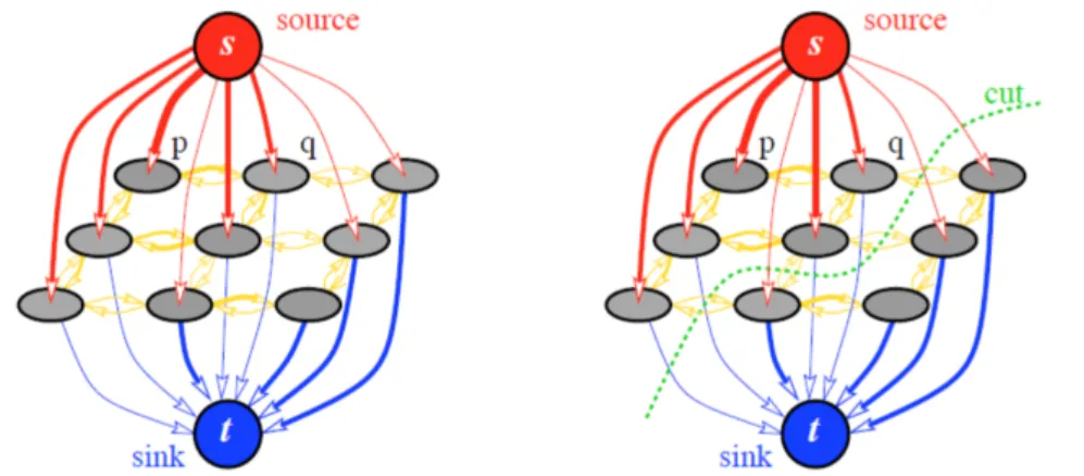
Figure 2.1: An example of graphs min-cut used for computer vision applications. Left is the graph constructed and the right is the min-cut result.
costs in comparison with learning max-flow from scratch.
2.1.2
Max-flow Applications
As various real world problems can be abstracted into max-flow prob-lems, or equivalent problems such as min-cut, there are vast applica-tions of max-flow. The bottleneck identification for a city traffic net-work Shengwu & Yi (2011) is a known max-flow application in which a traffic network in a city is abstracted into a road graph. Applying max-flow computation on the road graph, a road with its total capac-ity taken to carry flow is considered as a bottleneck. Similarly, bottle-neck identification for a power system has been used for computing a power system security index Kosut (2014) in which power supply links are represented as edges, and factories or towns are denoted as nodes. Max-flow is also applied in a wireless mobile environment to optimize the association between wireless clients to access points by maximizing the traffic flow to clients Dandapat et al. (2010) Dandapat et al. (2012) Li et al. (2014).
Max-flow/min-cut has also been widely used in computer vision, particularly for energy minimization problems such as image segmen-tation Duan et al. (2012) Weglinski & Fabijanska (2012) Boykov & Funka-Lea (2006) Boykov & Funka-Funka-Lea (2004), restoration Boykov & Jolly (2001) Lerm´e et al. (2014), stereo image processing Boykov et al. (1998) Shade & Newman (2011) Isack & Boykov (2014) Greig et al. (1989), shape reconstruction Snow et al. (2000) Paris et al. (2006) Yu et al. (2006) Labatut et al. (2007), object recognition Boykov & Huttenlocher (1999) Suga et al. (2008) Ladicky et al. (2010), augmented reality Thirion et al. (2000) Mooser et al. (2007) Tian et al. (2010), and texture syn-thesis Kwatra et al. (2003) Gracias et al. (2009). For a comprehen-sive overview of max-flow/min-cut applications in computer vision, please refer to Boykov & Kolmogorov (2004). The graphs used for these typically have a specific structure, and the goal is to assign one of two labels to every pixel in an image.
The graph in these applications is generated based on a regular 2D grid where each node, except the source and the sink, represents an image pixel. The adjacent nodes are usually pixels that are adjacent in the corresponding image, as shown in the left part of Figure 2.1. The source and sink nodes, which are also known as the terminal nodes, are two special nodes. They represent the two possible labels which can be assigned to all the other nodes (i.e., pixels in the image). The terminal nodes are connected to all the other nodes with varying ca-pacities Greig et al. (1989) Kolmogorov & Zabih (2001) Kolmogorov & Zabih (2002).
The edge capacities between adjacent non-terminal nodes are set according to a penalty for discontinuity between the pixels associated with these nodes. They represent how well a label from one pixel would continue into the adjacent pixel. The edge capacities between the terminal nodes and the non-terminal nodes are set according to a penalty for assigning the corresponding label to the pixel. When this graph is generated, the s− t min-cut on the graph is used for label
assignment. As shown in the right side of Figure 2.1, after the min-cut, nodes (pixels) connected with the source node s are labeled as one class and the others are labeled as another class.
Similar to its application in computer vision, min-cut is also ap-plied to find clusters in various types of networks, which can be eas-ily mapped to a graph, such as biological and sociological networks Raj & Wiggins (2010). The Information Bottleneck (IB) method Tishby et al. (2000) Tishby & Slonim (2001), developed based on rate distor-tion theory Shannon (2001), is representative of this track. It has been adopted in applications such as clustering word documents and gene expressions Slonim (2002) Slonim & Tishby (2000), identifying mod-ularity in synthetic and natural networks Ziv et al. (2005), classifying galaxies by their spectra formation Slonim et al. (2001), and commu-nity detection in social networks Mu et al. (2013) Papadopoulos et al. (2012) Ruan et al. (2013).
The applications of incremental max-flow, on the other hand, focus on learning in the changing environment. Grundmann et al. adopt incremental max-flow for image segmentation in continuous video frames Grundmann et al. (2010). A video can be seen as a series of images, so that each frame has little difference in comparison with the last frame. In this case, the graph constructed for image segmenta-tion also has minor differences between neighboring frames. Thus the incremental learning of graph Gi+1 based on the max-flow result of graph Gi, better suits this scenario in comparison with learning Gi+1 from scratch. In this sense, incremental max-flow can be naturally applied to various computer vision tasks introduced before, for learn-ing from video frames. Moreover, in the works Saha & Mitra (2006) and Zhou et al. (2010), incremental max-flow is employed for graph-based clustering in dynamic settings, in which the graph represents real-world data that are changing continuously over time.
2.2
Batch Max-flow Algorithms
In solving max-flow problems, existing algorithms fall into two cat-egories, namely preflow push method and augmenting path method Kleinberg & Tardos (2005). Existing batch max-flow algorithms are introduced in this section.
2.2.1
Augmenting Path
Augmenting path Ford & Fulkerson (1956) algorithm stores informa-tion about the distribuinforma-tion of the currents−tflowF among the edges ofGusing a residual graphR = (V, E, R). The topology ofRis identi-cal toG(i.e.,GandRshare the sameV andE), butR(e), the capacity of edge e in R, reflects the residual capacity of the same edge in G given the amount of flow already in the edge. At the initialization, there is no flow from the source to the sink (F = 0) and edge capac-ities in the residual graph R are equal to the original capacities in G (i.e.R(e) =C(e),∀e∈E).
Augmenting path algorithm is an iterative procedure of the fol-lowing two steps:
1) Find s−t path using Breadth-First Search (BFS). The resulting path P is a set of edges with positive residual capacity laid end to end connecting s to t, such as P = {(s, u),(u, v),(v, t) | R(s, u) >
0, R(u, v)>0, R(v, t)>0}.
2) Augment thes−tpath found above. We firstly find the maxi-mum amount of flow that can go through this pathP, which is termed augmentation value and denoted as∆P in the rest of this work. As it
is a bottleneck problem here, ∆P can be calculated as the minimum
residual capacity of the whole path∆P = min(R(u, v) | ∀(u, v) ∈ P).
Next, we send∆P flow through pathP inRas, R(u, v) = R(u, v)−∆P,∀(u, v)∈P R(v, u) = R(v, u) + ∆P,∀(u, v)∈P
The above two steps are iteratively executed until no more s −t paths can be found. Figure 2.2 gives an example of max-flow search through the augmenting path algorithm.
2.2.2
Boykov-Kolmogorov (BK) Algorithm
The BK algorithm Boykov & Kolmogorov (2004) is developed based on the augmenting path method. It has been extensively utilized by the computer vision community, since it is superior in practice to oth-ers on many vision instances Goldberg et al. (2015).
A difference from standard augmenting path algorithm, which finds thes−tpath via a single BFS search starting from source nodes, the BK algorithm seeks thes−tpath in a bi-directional manner.
The BK algorithm maintains two non-overlapping search trees S and T rooted at s and t respectively. In S, all edges from parents to children have positive residual capacity; and inT, all edges from children to parents have positive residual capacity. Nodes in G but not inS orT are termed as free nodes, and the nodes inS andT are either active (the outer boundary of each tree) or passive (the internal points of each tree). Figure 2.3 gives an example of the trees.
In the initial state, S has only one node s and T only contains t. Then the BK algorithm iteratively conducts operations in three stages: growth, augmentation, and adoption.
At the growth stage, the two search trees are expanded to find the s−tpath. Each active node explores adjacent edge with positive resid-ual capacity (R(u, v) > 0 foru ∈ S, and R(v, u) > 0for u ∈ T ), and adds newly discovered free nodes into the tree as its children. The newly added nodes are set as active. When all neighbors of an active node have been scanned, the active node is set to be passive. If no ac-tive node remains, the whole BK algorithm terminates. If a edge from S toT is found, which means there is as−t path, the augmentation
(a)
(b)
(c)
(d)
Figure 2.2: An example of max-flow search through augmenting path. (a) initial residual graph with the first founds−tpath shown in dot-ted lines; (b) augmendot-ted residual graph with newly founds−t path; (c) current augmented residual graph, where augmenting path termi-nates since no more s−t path can be found; (d) the obtained actual max-flow.
Figure 2.3: An example of treesS andT in BK algorithm. Non-active and active nodes are marked as blue and red respectively.
Figure 2.4: An example of the search treesS (red nodes) andT (blue nodes) at the end of the growth stage when a path (yellow line) from the source s to the sink t is found. Active and passive nodes are la-beled by letters A and P, correspondingly. Free nodes appear in black. stage starts. Figure 2.4 gives an example of whenSmeetsT at the end of the growth stage.
At the augmentation stage, thes−tpath found in the growth stage is augmented by sending maximum possible flow through it. After the augmentation, some edges on the augmenting path become satu-rated (i.e., residual flow becomes zero). Thus some nodes inS and T become orphans, as the edges linking them to their parents are satu-rated. If edge(u, v)becomes saturated and bothuandvare originally
Figure 2.5: An example of adoption step on a nodev. An orphan sub-tree is shown in the triangle. The solid edges are residual edges which are tree edges and the dashed edges are residual edges which are not tree edges. Nodeu can be selected as a parent ofv. But w cannot be selected as a parent forv, because there is no residual path fromwto t(the path terminates atv).
in tree S, then v becomes a S-orphan. If both u and v are originally in treeT, thenubecomes a T-orphan. If uis inS and v is inT, then no orphan is created in(u, v)saturation. In the other words, the aug-mentation operation may split treesSandT into forests, wheresand t are still the root of S andT respectively, and the orphans form the roots of all other trees. Orphans created in the augmentation stage are placed in a list and handled in the adoption stage.
In the adoption stage, orphans are processed until there are no or-phans left. The BK algorithm tries to find a new valid parent inS for each S-orphan, and similarly a parent in T for each T-orphan. For instance, if we have aS-orphanv, we seek suchuthat hasR(u, v)>0, u ∈ S and the tree path fromstouis valid (the whole path has posi-tive residual capacity). If such auis found, we makeuto be the parent ofv. If we cannot find a new parent forv, we markvas a free node and
mark all former children ofv as orphans. Then we examine all edges
(u, v)have positive residual capacity, and make eachu∈ Sactive. When the adoption stage is complete, the algorithm returns to the growth stage. The algorithm terminates whenS and T cannot grow (i.e., there are no active nodes) and the trees are separated by saturated edges (i.e., with zero residual capacity).
2.2.3
Incremental Breadth First Search (IBFS) Algorithm
The IBFS algorithm Goldberg et al. (2011) Hed (2011) is a modifica-tion of the BK algorithm, where theS and T trees are maintained to be always breadth-first trees. As a result, anys−tpath found in the procedure is a shortest path, and the overall running time has a poly-nomial boundO(n2m).The IBFS algorithm also maintains two trees S and T, which are rooted atsandtrespectively. At any given moment, a node can be in one of five states: S-node, T-node, S-orphan, T-orphan, or N-node (which indicates the node is not in any tree). There is a parent pointer for each node indicating the parent of this node in the tree, which is empty for N-nodes and orphans. A node u is called in S if u is a S-node or aS-orphan.
Distance labelsds(u)ordt(u)are maintained for each nodeu,
rep-resenting the distance fromsorttouin the tree. Ifuis inS, then only ds(u)is meaningful anddt(u)is unused. The situation for nodes in T
are symmetric. For some valuesDs andDt, the nodes in treeS have
no more thanDsfromsand the nodes in treeT have up toDtdistance
tot. ThusL = Ds+Dt + 1 is the lower bound of the length of any
augmenting path.
Similar to the BK algorithm, IBFS also has three steps: growth, augmentation, and adoption. At the initial state, S has onlys, T has onlyt,ds(s) =dt(t) = 0, and parent pointers for all nodes are empty.
Figure 2.6: An example of a forward pass of IBFS. Note that during a forwardS grown pass, active nodes exist only in levelDsofS.
there are no orphans. All nodes inSareS-nodes, all nodes inT areT -nodes, and the rest nodes areN-nodes. In a pass of the growth stage, IBFS chooses a tree to grow (forward forS and backward for T) for one level, this increasesDs (orDt) andLby one. Figure 2.6 gives an
example.
Taking a forward growth pass as an example, in which tree S is grown, the operation for a backward pass is symmetrical. Firstly, all nodes u inS with ds(u) = Ds are set to be active. The pass then
ex-ecutes growth steps. This may be interrupted by augmentation steps (when an augmenting path is found) followed by adoption steps (to fix the invariants violated when some arcs get saturated). At the end of the pass, ifS has any nodes at levelDs+ 1,Dsis incremented by1;
otherwise the algorithm terminates.
The growth step picks an active nodevand scans all residual edges
(v, w)leavingv. Ifwis aS-node, nothing is done about it. Ifwis aN -node, we markwas aS-node, setp(w) =v, and setds(w) =Ds+ 1. If wis inT, an augmentation step is performed. Once all residual edges
Figure 2.7: An example of augmentation step of IBFS. The parent edges of the orphan nodes are saturated during this augmentation. The triangles represent the orphan sub trees that are created after the augmentation. Note the augmenting path is always a shortest s −t path in the residual graph.
leaving v are scanned, v becomes inactive. If the scan on v is inter-rupted by augmentation, we record the outgoing residual edge that triggered the augmentation. Ifv is still active after the augmentation, the scan ofv is resumed from that edge.
The augmentation step is performed when a residual edge (v, w)
is found such thatv is in S and w is inS, as shown in Figure 2.7. In such circumstances, the pathP obtained by connecting thesvpath in S, the edge (v, w), and the wt path in S is an augmenting path. We conduct augmentation onP, saturating some of its edges. Saturating any arc(x, y)other than (v, w)creates orphans. Note thatxand yare in the same tree. If they are both inS, y is marked as an S-orphan, otherwisexis marked as aT-orphan. At the end of the augmentation step, there are two sets (possibly empty) ofS-orphans andT-orphans.
Figure 2.8: An example of adoption step of IBFS, in which orphan v is relabeled. The solid edges are residual edges which are tree edges. The dashed edges are residual edges which are not tree edges. The triangles represent orphan sub trees. Node v finds u as the lowest potential parent and performs a relabel withuas his new parent. The children ofv then become orphans themselves and will be processed later during this adoption phase.
These sets are handled during the adoption step.
The adoption step recovers the S and T trees by eliminating or-phans, Figure 2.8 gives an example. Here we assume S is grown thus we have S-orphans to be processed. The adoption procedures for eliminatingT-orphans are symmetric. To process anS-orphanv, the edges list is scanned starting from the current edge and the scan stops when a residual edge(u, v)with ds(u) = ds(v)−1is found. If
such a uis found, v is marked as anS-node, the current edge of v is set to be (v, u), and u is set to be the parent ofv. If such a u cannot be found, the orphan relabelling operation is applied tov. This rela-bel operation scans the whole edge list to find the u such that ds(u)
is minimum and(u, v)has positive residual capacity. If no suchu ex-ists, or ifds(u) > Ds, we makev as aS-node and mark nodeswsuch
that p(w) = v as S-orphans. Otherwise we choose u to be the first such node and set the current edge ofv to be(v, u), set p(v) = u, set ds(v) = ds(u) + 1, make v an S-node, and mark nodes w such that p(w) = v asS-orphans. If v was active and now hasds(v) = Ds+ 1,
we makevinactive.
2.2.4
Push Relabel Algorithm
The push relabel algorithm is also known as the preflow push algo-rithm, which was developed by Goldberg and Tarjan Goldberg & Tar-jan (1988). Different from algorithms in augmenting path family, the push relabel algorithm does not keep the mass balance constraint hold at all times. The graph is flooded with excesses in the push relabel al-gorithm, these excesses are either pushed towards sinktto form actual s−tflow, or pushed back to sourcesfor those that cannot reachtto satisfy the mass balance constraint at the end of algorithm execution.
Excesse(v)at a node v is defined as the amount of incoming flow that exceeds the outgoing flow
e(v) = X
(u,v)∈E
f(u, v)− X (v,w)∈E
f(v, w). (2.3) A node with positive excess is termed as an active node. In order to es-timate the distance of a node fromsort, distance labeldis maintained for each node. For sourcesand sinkt, we haved(s) =nandd(t) = 0. For any edge(u, v)in the residual graph, we haved(u)≤d(v) + 1.
The push relabel algorithm consists of two basic operations: push and relabel. The push operation pushes the largest possible amount of
flow through an admissible edge, the procedure of the push operation is given in Algorithm 1. Note that line1in Algorithm 1 is the condition test to see if edge(u, v)is admissible for the push operation.
Algorithm 1Push Operation in Push Relabel Algorithm
Input: GraphG = (V, E, C), residualR, distance labelingd, excesse,
and the edge to push(u, v).
Output: GraphG= (V, E, C), residualR, distance labelingdand
ex-cesse.
1: ife(u)>0,R(u, v)>0andd(u) =d(v+ 1).then
2: Sendδ =min(e(u), R(u, v))amount flow through edge(u, v)as: R(u, v)←R(u, v)−δ;R(v, u)←R(v, u) +δ;
e(u)←e(u)−δ;e(v)←e(v) +δ.
3: end if
Relabel is another basic operation in the push relabel algorithm. When there is no admissible edge to push, the relabel operation ad-justs distance labels to make the push operation possible again. This procedure is stated in Algorithm 2. Note that line1in Algorithm 2 is the applicability test for relabelingu.
Algorithm 2Relabel Operation in Push Relabel Algorithm
Input: GraphG = (V, E, C), residualR, distance labelingd, excesse,
and the node to relabelu.
Output: GraphG= (V, E, C), residualR, distance labelingdand
ex-cesse.
1: ife(u)>0and∀R(u, v)>0haved(u)≤d(v).then
2: Relabeld(u) =min(d(v) :R(u, v)>0) + 1.
3: end if
At the initial state of the push relabel algorithm, the residual graph is identical to the input graph, the distance labeling isn for source s
and 0 for all other nodes, the source node has infinite excesses. The algorithm starts with a set of initial saturating pushes, in which each edge(s, u)leaving sourcesis pushed with a flow that equals its capac-ityC(s, u). Then the algorithm repeatedly performs push and relabel operations to push excesses and modify distance labeling. For a push on (u, v), δ = min(e(u), R(u, v)) flow is pushed from u to v, which increasesR(v, u) and e(v)by δ and decreasesR(u, v)and e(u) by the same amount. For a relabel onu, the distance labeld(u)is set to be the largest value allowed by the valid labeling constraint. The algorithm terminates when there is no active node left. At this point, none of the nodes exceptsand t have excesses, thus the mass balance constraint is satisfied and the preflow becomes flow, which is the max-flow ob-tained.
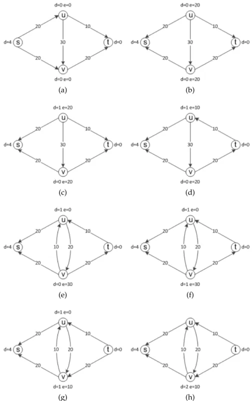
An example of push relabel execution is given in Figures 2.9 and 2.10. Figure 2.9a shows the input residual graph and distance labeling, the residual graph is identical to input graph at this state. In Figure 2.9b, the initial saturating push is conducted over all edges leaving sources,20flows are pushed through (s, u)and (s, v). In Figure 2.9c, active nodeuis relabeled, so that it can push its20excesses towards sink t and nodev. The excesses onu are pushed through edge (u, t)
and (u, v) in Figures 2.9d and 2.9e, respectively. In Figure 2.9f, the active node v is relabeled, so that it can push excesses towardst. In Figure 2.9g,20excesses onv are pushed totvia(v, t). In Figure 2.9h, the active nodev is relabeled as d(v) = 2, so that edge(v, u)becomes admissible.
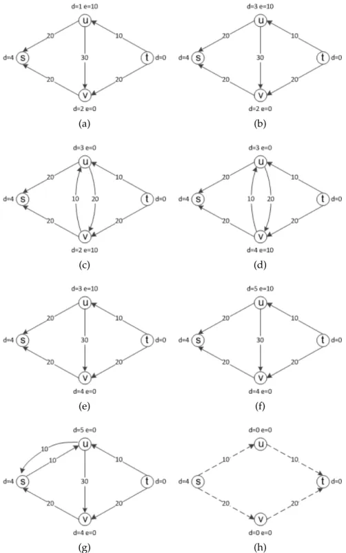
In Figure 2.10a, the remaining 10 excesses on v are pushed to u. At this state, there are two edges(u, s)and(u, v), leaving active node u with positive capacity. Since d(s) = 4 and d(v) = 2, u is relabeled asd(u) = 3 in Figure 2.10b. Then the excess onu is pushed to v via admissible edge(u, v)in Figure 2.10c. Next, in Figure 2.10d nodev is relabeled asd(v) = 4and the excess onv is pushed tou.
(a) (b)
(c) (d)
(e) (f)
(g) (h)
Figure 2.9: An example of max-flow search through push relabel. Part A
(a) (b)
(c) (d)
(e) (f)
(g) (h)
Figure 2.10: An example of max-flow search through push relabel. Part B
The steps of push relabel algorithm are summarized in Algorithm 3.
Algorithm 3Push Relabel Algorithm
Input: GraphG= (V, E, C).
Output: GraphG= (V, E, C), residualR, distance labelingdand
ex-cesse.
1: Initialize residual graph asR(u, v) = C(u, v),∀(u, v)∈E;
2: Initialize distance label asd(s) = nandd(u) = 0,∀u∈V \ {s};
3: Initialize excess ase(s) =∞ande(u) = 0,∀u∈V \ {s};
4: forEach(s, u)thatC(s, u)>0do
5: PushC(s, u)through(s, u)as:
e(u) =C(s, u),R(s, u) = R(s, u)−C(s, u)and R(u, s) = C(u, s) +C(s, u);
6: end for
7: whileThere exists a basic operation that appliesdo
8: Select a basic operation and perform it;
9: end while
2.3
Incremental Max-flow Algorithms
Based on the above batch algorithms, some incremental max-flow al-gorithms are propose for learning from dynamic graphs. In this sec-tion, we review the most important incremental max-flow algorithms.
2.3.1
Incremental Push Relabel
Kumar and Gupta Kumar & Gupta (2003b) propose an incremental max-flow algorithm based on the push relabel mechanism. In their incremental push relabel algorithm, graph change is considered as serting and deleting of edges which is equivalent to edge capacity
in-crease and dein-crease. These changes are addressed on one edge after another.
For any edge inserting or deleting, the incremental push relabel algorithm first finds the set of nodes that are affected by this change. In the case of inserting a new edge u, v, the possible newly formed flow will go through augmenting paths from source s to u and then v to sink t. The first set of affected nodes, which lie on the path of s tou, are found by Backward Breadth First Search (BBFS) fromuto s, and the second set of affected nodes, which lie on the path of v tot, are found by Forward Breadth First Search (FBFS). On the other hand, when an edgeu, vis deleted, some existing augmenting pathes go throughs−u−v−tmay be affected. Thus the affected nodes are found by BBFS from u tos and FBFS from t tov. The algorithms of BBFS and FBFS are given in Algorithms 4 and 5, respectively.
Algorithm 4Backward Breadth First Search Algorithm
Input: GraphG= (V, E, C), start nodeu, end nodev.
Output: Affected node setAF F.
1: InitializeW ORKSET ={u};
2: InitializeAF F ={u};
3: whileW ORKSET 6=∅do
4: Remove an elementxfromW ORKSET;
5: ifx=v then
6: else
7: forall edges(y, x)∈Edo
8: ifC(y, x)>0then 9: AF F =AF F ∪ {y}; 10: W ORKSET =W ORKSET ∪ {y}; 11: end if 12: end for 13: end if 14: end while
Algorithm 5Forward Breadth First Search Algorithm
Input: GraphG= (V, E, C), start nodeu, end nodev.
Output: Affected node setAF F.
1: InitializeW ORKSET ={u};
2: InitializeAF F ={u};
3: whileW ORKSET 6=∅do
4: Remove an elementxfromW ORKSET;
5: ifx=v then
6: break
7: else
8: forall edges(x, y)∈Edo
9: ifC(x, y)>0then 10: AF F =AF F ∪ {y}; 11: W ORKSET =W ORKSET ∪ {y}; 12: end if 13: end for 14: end if 15: end while
Based on the push relabel algorithm discussed in Section 2.2.4, Ku-mar and Gupta give two lemmas that are important to help identify affected nodes:
2.1.LEMMA. For any nodeuin the result of push relabel algorithm, if have
d(u)< n, then no extra flow can be sent from sourcesto the nodeu.
2.2.LEMMA. For any nodeuin the result of push relabel algorithm, if have
d(u)≥n, then no extra flow can be sent from the nodeuto sinkt.
The proof of Lemmas 2.1 and 2.2 can be found in study Kumar & Gupta (2003b).
Edge Insertion
For a newly inserted edge(u, v), Kumar and Gupta’s algorithm firstly finds affected nodes and then uses the basic push relabel operation within the affected nodes (which is normally a subset of the whole graph) to find the newly formed s −t flow. In finding the affected nodes, the following interpretation is given.
1. Each newly formed flow must start fromsand passuon its way tot. Flows that do not lead to u and t are useless as they will return to the sources.
2. According to Lemma 2.1, on the way fromstou, only the nodes x that have d(x) ≥ n are candidates for being affected nodes, because for those nodesythat haved(y)< ncannot receive extra flow froms.
3. According to Lemma 2.2, on the way fromv tot, only the nodes x that have d(x) < n are candidates for being affected nodes. This is because for those nodesythat haved(y)≥ncannot send extra flow tot.
4. Only edges(x, y)that have positive residual capacityR(x, y)>0
can route extra flow after(u, v)insertion.
Based on these four points, the identification of affected nodes in the case of edge(u, v)insertion consists two steps:
1. Add two extra conditions thatd(x) ≥nandR(x, y)>0at line9
of Algorithm 4. Call above modified BBFS Algorithm to search fromutos.
2. Add two extra conditions thatd(x)< nandR(x, y)>0at line9
of Algorithm 5. Call above modified FBFS Algorithm to search fromvtot.
Having identified all affected nodes, the incremental push relabel algorithm then initializes the preflowf as:
1. The residual capacity for each edge leaving source nodesto an affected node.
2. Zero for any other edges (between affected nodes and sinkt). This preflow initialization is followed by a modified push relabel op-eration, in which the push and relabel process only applies to those affected nodes.
The incremental push relabel algorithm terminates when there are no more active nodes in the graph. At this point, if there is any new flow formed due to the insertion of(u, v), the new flow is found and added into the current flow. The steps for the incremental push relabel algorithm to handle edge insertion are stated in Algorithm 6.
Algorithm 6Incremental Push Relabel - Edge Insertion
Input: Graph G = (V, E, C), residual graph R, edge (u, v) to be
in-serted.
Output: Residual graphR.
1: Call Algorithm 4 to conduct BBFS fromutos;
2: Call Algorithm 5 to conduct FBFS fromv tot;
3: Initialize distance label asd(s) = nandd(u) = 0,∀u∈V \ {s};
4: Initialize excess ase(s) =∞ande(u) = 0,∀u∈V \ {s};
5: forEach(s, u)thatR(s, u)>0do
6: PushR(s, u)through(s, u)as:
e(u) =C(s, u),R(s, u) = R(s, u)−C(s, u)and R(u, s) = C(u, s) +C(s, u);
7: end for
8: whileThere exists a basic operation that appliesdo
9: Select a basic operation and perform it;
Edge Deletion
For an edge(v, w)removed from the original graph, there is a possibil-ity of changing the max-flow only when there is flow through(v, w). In this case, when (v, w)is deleted, the flow f(v, w) on this edge be-comes zero and this amount of flow must be pushed back from t to wand then tov. Then the excess onv is pushed as much as possible towardstusing alternate augmenting paths in the modified graph. If there is some excess onv that cannot be pushed tot, it will be pushed back tos.
In the incremental push relabel algorithm, nodesvandware set as active. The algorithm tries to push excesses towardsandt, in which there are three operations to be performed:
1. Pushing flow fromttow; 2. Pushing flow fromwtov; and
3. Pushing flow fromvandwtowardstands.
For the first operation, which is a preflow push problem in the reversed direction, a reverse graph GR is used. GR is obtained by
reversing all the residual edges in graphG. Since not all nodes inGR
are associated with the flow fromttow, the FBFS algorithm is called with argumentsw and t to find the affected nodes. Then a standard push relabel algorithm is applied on these nodes to push flow fromt tow.
Once the first operation is finished, f(v, w) amount of excess is pushed fromw tov. After this pushing, edge(v, w)can be safely re-moved since no flow goes through it.
When these first two operations are accomplished, nodevhasf(v, w)
amount of excesses, which are pushed from w in step 2 and node w may have some excess as well. This is because over f(v, w)amount of flow is pushed fromttowin step1, as the push relabel algorithm,
different from the augmenting path algorithm, cannot control the total amount of flow pushed.
For the third operation, the algorithm conducts two separate push relabel procedures with active nodesv andw. The complete steps for the incremental push relabel algorithm to handle edge deletion are stated in Algorithm 7.
Algorithm 7Incremental Push Relabel - Edge Deletion
Input: Graph G = (V, E, C), residual graph R, edge (v, w) to be
deleted.
Output: Residual graphR.
1: Reverse residual graphR, obtainGR
2: Call Algorithm 5 to conduct FBFS fromttow;
3: Call Algorithm 3 to push from t tow inGR, with constraint that all operations are applied in affected nodes;
4: Pushf(v, w)excess fromwtovinR
5: Delete(v, w)fromGandR;
6: Call Algorithm 5 to conduct FBFS fromv tot;
7: Call Algorithm 3 to push fromvtotinGR, with constraint that all
operations are applied in affected nodes;
8: Call Algorithm 5 to conduct FBFS fromwtot;
9: Call Algorithm 3 to push from wto t inGR, with constraint that
all operations are applied in affected nodes;
2.3.2
Excesses IBFS Algorithm
The excesses IBFS (EIBFS) algorithmGoldberg et al. (2015) was devel-oped based on the IBFS algorithm and is capable of learning max-flow from dynamic graphs.
On Static Graphs
Different from IBFS and BK, in which a feasible flow is always main-tained, EIBFS is a generalized IBFS that maintains only a pseudoflow. Pseudoflow is a flow that follows the capacity constraint, but not con-servation constraints.
A nodev is known as an excess ife(v)>0and a deficit ife(v)<0. In EIBFS, source s and sink t are defined to has infinite excess and deficit, respectively. EIBFS maintains two node-disjoint forestsS and T. Each excess is a root of a tree inS, and a root of tree inS must be an excess. Similarly, each deficit is a root of a tree inT, and a root in T must be a deficit. For a non-root nodevinS orT,p(v)is the parent ofvin its respective forest. A node which is not inS nor inT is called a free node.
EIBFS also maintains distance labelsds(v)anddt(v)for every node v, just as in IBFS. The edges in forests S and T are admissible with respect todsanddt, respectively.
Initially, every rootrinSor inT hasds(r) = 0ordt(r) = 0,
respec-tively. But new excesses and deficits formed in the algorithm execu-tion may have arbitrary distance labels. Thus the roots of a tree do not necessarily have a zero distance label. Similar to that in IBFS,Ds and Dtare maintained as
Ds = maxv∈S(ds(v)) Dt = maxv∈T(ds(v)).
(2.4) At the initial state of EIBFS, S has only s, S has only t, ds(s) = dt(t) = 0,Ds =Dt = 0andp(v)is empty for every nodev. The EIBFS
algorithm is executed in phases. Each phase is either a forward phase (when theS forest is grown) or a backward phase (when theT forest is grown). Every phase first performs the growth steps, which may be interrupted by augmentation steps (when an augmenting path is found) and followed by alternating adoption and augmentation steps. Using the forward phase as an example to describe the procedures
of EIBFS, the procedures in the backward phase are symmetric. For a forward phase, the goal is to grow forest S by one level. If S has nodes at level Ds + 1 at the end of the phase, Ds is incremented by
one; otherwise the algorithm terminates.
In the forward phase, growth steps are performed first. All nodes vinSthat hasds(v) = Dsare marked as active. Then we pick an active
nodevand scan v by examining all residual edges(v, w)leavingv. If w∈ S, we do nothing. Ifwis a free node, we addwtoS, setp(w) =v, and setds(w) =Ds+ 1. Ifw∈ T, which means an augmentation path
fromstotis found, the augmentation step is performed as described later. Edge(v, w)is recorded as the outgoing edge that triggered the augmentation step. Ifv is still active after the augmentation step, the scan ofv is resumed from (v, w) to avoid re-scanning the edges that were processed. If (v, w) is still residual and connects the forests, we do more augmentation steps using it. After all edges out of v have been scanned, v becomes inactive. When all nodes are inactive, the phase ends.
The augmentation steps in EIBFS are different from those in IBFS. When a connecting edge(v, w)that hasv ∈ S andw∈ S is found, we increase the flow on(v, w)by any feasible amount without violating the capacity constraint of(v, w). As a result of the flow that is added, an excess may be created inT and a deficit may be created inS. We now alternate between augmentation steps and adoption steps, as de-scribed below. Once all excesses have been drained or removed from T and all deficits have been drained or removed fromS we continue to perform growth steps.
We now introduce how to handle excesses created inT, the deficits inSare addressed symmetrically. A nodevinT is called an orphan if its parent arc(v, p(v))is not admissible (possibly saturated) and have e(v)≥ 0. An augmentation step is executed by picking an excessv in T and pushing flow out ofv, as described below. This push may cre-ate orphans and more excesses inT. If orphans are created, adoption
steps are performed to repair them. After orphans are repaired, we ex-ecute another augmentation step from another excess. Augmentation and adoption steps stop when all excesses are drained or removed fromT.
Flow is pushed out of an excess v inT as follows. The tree path from v to the root r inT are traversed. For every edge (x, y)in this path, we increase its flow by minR(x, y), e(x). This means that we either drain the entire excess fromxor saturate the edge(x, y), making xan orphan. Rootr remains a deficit if not enough excess is drained into it. Otherwise it hase(r) ≥ 0and becomes an orphan, thus it can no longer serve as a root inT.
In the adoption step, an orphanv inT is repaired by either setting a new parent p(v)inT or by removing v from T. The adjacency list ofv is scanned starting from the current arc and scanning stops when an admissible outgoing edge is found or the end of the list is reached. If an admissible edge(v, u)is found, we set the current arc ofv to be
(v, u)and set p(v) = u. If no such edge can be found, we apply the orphan relabel operation tov.
The orphan relabel operation scans the adjacency list ofv to find a new parentuforv. A nodeuis qualified to be a new parent ofv if: 1) uis a node with minimumdt(u)such that(v, u)has positive residual
capacity; and 2) dt(u) < Dt for a forward phase, ordt(u) ≤ Dt for a
backward phase. If such au is found (there may be more than one), we set the first such node to beu, set the current edge ofv to be(v, u), setp(v) = uand set dt(v) = dt(u) + 1. As a result, every nodewwith p(w) =v becomes an orphan. These new orphans need to be repaired by adoption steps. If no such u is found, we make v a free vertex if e(v) = 0or addv toS as a new root ife(v)>0.
On Dynamic Graphs
The EIBFS algorithm considers graph changes as violations to flow feasibility or to the invariants of the algorithm. The violations are
summarized as following types:
a) An edge (v, w) such that f(v, w) > C(v, w), due to edge capacity reduces;
b) A new residual edge(v, w)such thatv ∈ Sandw∈ T;
c) A new residual edge(v, w)such thatvandware inShavingds(w)> ds(v) + 1, or the symmetric case in treeT;
d) A new residual edge (v, w) such that v and w are in S, ds(w) = ds(v) + 1, and(v, w)precedes the current arc ofv, or the symmetric
case in treeT;
e) A new residual edge(v, w)such thatv ∈ S,ds(v)≤Dsandwis not
inS, or the symmetric case in treeT.
These violations are fixed by some base operations introduced in the static graph setting. Specifically, (a) is resolved by pushing flow along(w, v); and (b), (c), and (e) are fixed by saturating edge(v, w). In these cases, new excesses or deficits are generated. These excesses and deficits are solved by alternating augmentation and adoption steps. The violation (d) is handled by simply reassigning the current arc of v.
2.4
Summary
Based on the above observations, we find that handling edge capac-ity reduction or edge removal (i.e., the decremental learning) is the most difficult part of incremental max-flow. This is because, this op-eration needs to redirect current flow in alternative paths or cancel current flow if it cannot be redirected. The performance of an incre-mental max-flow is determined, to a large extent, by its decreincre-mental operation.
We also found that both existing incremental max-flow algorithms apply push-relabel style operation in handling edge capacity reduc-tion. This method involves a great amount of operations in neighbor search, flow push and node relabel, thus has higher empirical compu-tational complexity.
Alternatively, we decided to derive an incremental max-flow algo-rithm based on the augmenting path mechanism. In the next chapter, we introduce the proposed augmenting path based on the incremental max-flow algorithm.
Chapter 3
Proposed Incremental Max-flow
Algorithm
3.1
Introduction
In this chapter, we present the proposed incremental max-flow algo-rithm which is constructed based on the augmenting path algoalgo-rithm. The augmenting path mechanism is introduced first. Then we derive the max-flow updating procedures in response to all possible graph changes.
For the convenience of algorithm derivation and clarity of presen-tation, we summarize most notations used in this chapter in Table 3.1.
3.1.1
Motivation
We address the max-flow problem because it is a fundamental algo-rithm in graph theory and can be used to solve various problems such as min-cut, multi-source multi-sink max-flow, maximum edge-disjoint path Kleinberg & Tardos (2005). Up to now, max-flow has been adopted in numerous real-world applications, such as bottle-neck identification for both city traffic network Shengwu & Yi (2011) and power system Kosut (2014). In the wireless mobile environment, max-flow is being applied to optimize the association between wire-less clients and access points by maximizing the traffic flow to clients Dandapat et al. (2010) Dandapat et al. (2012). In addition, it has been
Notation Descriptions G weighted graph,G= (V, E, C) V node set E edge set C capacity set u,v nodeu, nodev
s,t source node, sink node
e edgee
(u, v) edge from nodeuto nodev C(e),C(u, v) capacity on edgeeand(u, v)
R residual graph,R= (V, E, R)
R(e),R(u, v) residual capacity on edgeeand(u, v)
f(u, v) flow value on edge(u, v)
F net flow value,F =P
u∈V f(u, t)
P path
Table 3.1: Notations
widely used in computer vision for image segmentation Duan et al. (2012) Weglinski & Fabijanska (2012) Boykov & Jolly (2001), stereo Shade & Newman (2011) Isack & Boykov (2014), and shape recon-struction Snow et al. (2000).
In the era of big data, data is becoming available quickly in a se-quential manner, which requires systems to process data in real time. For max-flow learning, if a huge graph changes frequently over time, then it is obviously not efficient to always retrain max-flow from scratch. In incremental max-flow, existing algorithms apply push-relabel style operations to handle edge capacity reduce, which is the key compo-nent that determines performance. This push-relabel method involves a great amount of operations in neighbor search, flow push, and node relabel, thus it has higher empirical computational complexity. Note that max-flow has the solution of either push relabel or augmenting
path Kleinberg & Tardos (2005). Apparently, incremental max-flow via augmenting path is left as an open question.
3.2
Preliminary
3.1.DEFINITION. A flow onGis a real valued functionf()if the following conditions are satisfied:
f(u, v) = −f(v, u), ∀(u, v)∈V ×V; (3.1a) f(u, v)≤C(u, v), ∀(u, v)∈V ×V; (3.1b)
X
u
f(u, v) = 0, ∀v ∈V \ {s, t}. (3.1c)
Let net flow F = P
u∈V f(u, t)be the summation of flows into sinkt.
Then, the max-flow problem is to determine a flow fromstotwith the maximum net flowF. In the rest of this work, we denote the direction fromstotass−t.
The augmenting path algorithm stores information about the dis-tribution of the current s −t flow F among the edges of G using a residual graphR= (V, E, R). The topology ofRis identical toG(i.e., GandRshare the sameV andE), butR(e), the capacity of edgeeinR, reflects the residual capacity of the same edge inGgiven the amount of flow already in the edge. At the initialization, there is no flow from the source to the sink (F = 0) and edge capacities in the residual graph Rare equal to the original capacities inG(i.e.R(e) =C(e),∀e ∈E).
The augmenting path algorithm is an iterative procedure of the following two steps:
1) Find s−t path using Breadth-First Search (BFS). The resulting path P is a set of edges with positive residual capacity laid end to end connecting s to t, such as P = {(s, u),(u, v),(v, t) | R(s, u) >