Single-Channel Speech Enhancement Based on Deep Neural Networks

SINGLE-CHANNEL SPEECH ENHANCEMENT BASED

ON DEEP NEURAL NETWORKS

Zhiheng Ouyang

A thesis in

The Department of

Electrical and computer engineering

Presented in Partial Fulfillment of the Requirements For the Degree of Master of Applied Science

Concordia University Montr´eal, Qu´ebec, Canada

December 2019 c

CONCORDIA UNIVERSITY SCHOOL OF GRADUATE STUDIES

This is to certify that the thesis prepared By: Zhiheng Ouyang

Entitled: Single-Channel Speech Enhancement Based on Deep Neural Networks and submitted in partial fulfillment of the requirements for the degree of

Master of Applied Science (Electrical and Computer Engineering)

complies with the regulations of this University and meets the accepted standards with respect to originality and quality.

Signed by the final examining committee:

________________________________________________ Chair Dr. H. Rivaz ________________________________________________ External Examiner Dr. C.-Y. Su (MIAE) ________________________________________________ Internal Examiner Dr. H. Rivaz ________________________________________________ Supervisor Dr. W.-P. Zhu Approved by: ___________________________________ Dr. Y.R. Shayan, Chair

Department of Electrical and Computer Engineering

_______________ 20___ __________________________________ Dr. Amir Asif, Dean,

Faculty of Engineering and Computer Science

Abstract

Single-channel speech enhancement based on deep neural networks

Zhiheng Ouyang

Speech enhancement (SE) aims to improve the speech quality of the degraded speech. Recently, researchers have resorted to deep-learning as a primary tool for speech enhancement, which often features deterministic models adopting supervised training. Typically, a neural network is trained as a mapping function to convert some features of noisy speech to certain targets that can be used to reconstruct clean speech. These methods of speech enhancement using neural networks have been focused on the estimation of spectral magnitude of clean speech considering that estimating spectral phase with neural networks is difficult due to the wrapping effect. As an alternative, complex spectrum estimation implicitly resolves the phase es-timation problem and has been proven to outperform spectral magnitude eses-timation. In the first contribution of this thesis, a fully convolutional neural network (FCN) is proposed for complex spectrogram estimation. Stacked frequency-dilated convolu-tion is employed to obtain an exponential growth of the receptive field in frequency domain. The proposed network also features an efficient implementation that re-quires much fewer parameters as compared with conventional deep neural network (DNN) and convolutional neural network (CNN) while still yielding a comparable performance.

Consider that speech enhancement is only useful in noisy conditions, yet conven-tional SE methods often do not adapt to different noisy conditions. In the second contribution, we proposed a model that provides an automatic ”on/off” switch for

speech enhancement. It is capable of scaling its computational complexity under different signal-to-noise ratio (SNR) levels by detecting clean or near-clean speech which requires no processing. By adopting information maximizing generative adver-sarial network (InfoGAN) in a deterministic, supervised manner, we incorporate the functionality of SNR-indicator into the model that adds little additional cost to the system.

We evaluate the proposed SE methods with two objectives: speech intelligibility and application to automatic speech recognition (ASR). Experimental results have shown that the CNN-based model is applicable for both objectives while the InfoGAN-based model is more useful in terms of speech intelligibility. The experiments also show that SE for ASR may be more challenging than improving the speech intelligi-bility, where a series of factors, including training dataset and neural network models, would impact the ASR performance.

Related Publications

The work in this thesis led to the following research publications:

1. Zhiheng Ouyang, Hongjiang Yu, Wei-Ping Zhu, Benoit Champagne. A Fully Convolutional Neural Network for Complex Spectrogram Processing in Speech Enhancement. In ICASSP 2019-2019 IEEE International Conference on Acous-tics, Speech and Signal Processing (ICASSP). IEEE, 2019. [Chapter 2]

2. Zhiheng Ouyang, Wei-Ping Zhu, Benoit Champagne. Speech Enhancement with Information Maximizing Generative Adversarial Network. In ICASSP 2020-2020 IEEE International Conference on Acoustics, Speech and Signal Pro-cessing (ICASSP). IEEE, 2020., Submitted October 2019. [Chapter 3]

3. Zhiheng Ouyang, Hongjiang Yu, Wei-Ping Zhu, Benoit Champagne. A Deep Neural Network Based Harmonic Noise Model for Speech Enhancement. In Interspeech. 2018.

Contents

List of Figures ix

List of Tables xi

List of Abbreviations xii

1 Introduction: Deep Learning for Speech Enhancement 1

1.1 Neural network models for SE . . . 2

1.1.1 Input feature and output target . . . 3

1.1.2 Neural networks . . . 6

1.2 Training datasets and training strategy . . . 13

1.2.1 Speech dataset . . . 15

1.2.2 Noise dataset . . . 17

1.2.3 Training strategy . . . 18

1.3 SE Objective and evaluation . . . 19

1.3.1 Evaluation of intelligibility . . . 20

1.3.2 Evaluation of ASR performance . . . 21

1.4 Objective and organization of this thesis . . . 21

1.4.1 Objective of the thesis . . . 21

2 Single-Channel Speech Enhancement with Convolutional Network 23

2.1 Previous work . . . 23

2.1.1 Complex spectrogram processing by DNN . . . 23

2.1.2 Convolutional neural networks for speech enhancement . . . . 27

2.1.3 WaveNet framework . . . 30

2.2 Proposed fully convolutional neural network for speech enhancement 34 2.2.1 Dilated 2-d and 1-d frequency convolution . . . 34

2.2.2 Network architecture . . . 35

2.3 Performance evaluation . . . 38

2.3.1 Performance measure of speech quality . . . 38

2.3.2 Performance measure of keyword spotting . . . 41

2.4 Summary . . . 46

3 Signal-Channel Speech Enhancement with Generative Adversarial Network 48 3.1 Previous work . . . 48

3.1.1 Generative adversarial network . . . 48

3.1.2 The application of GAN in speech enhancement . . . 50

3.2 Proposed InfoGAN-based method for speech enhancement . . . 53

3.2.1 Introduction to InfoGAN . . . 53

3.2.2 Adopting InfoGAN for speech enhancement . . . 56

3.3 Performance evaluation . . . 62

3.3.1 Experimental setup . . . 62

3.3.2 Performance measure of speech quality . . . 63

3.3.3 Performance measure of keyword spotting . . . 69

4 Conclusion and Future Work 74

4.1 Summary of the work . . . 74 4.2 Suggestions for future work . . . 76

List of Figures

1 A DNN for CIRM estimation . . . 8

2 CNN with fully-connected layers and fully convolutional neural network 10 3 A comparison of SE performance of different network structures and their model size . . . 11

4 A Wavenet for SE . . . 11

5 A LSTM for CIRM estimation . . . 12

6 A VAE for SE . . . 13

7 A GAN for image inpainting task . . . 14

8 A DNN for LPS estimation . . . 25

9 The block diagram of DNN for LPS estimation . . . 26

10 Different representations of a clean speech signal . . . 28

11 A CNN for complex spectrogram estimation . . . 30

12 The network sturcture of RCED . . . 31

13 A FCN with autoencoder-decoder design . . . 31

14 Stacked dilated causal 1d convolution . . . 32

15 The network structure of WaveNet . . . 33

16 Stacked non-causal, dilated 1d convolution . . . 33

17 Frequency dilated 2-d convolution . . . 35

18 2d convolution an 1d convolution . . . 36

20 Average PESQ score on female and male speech by replacing phase . 39

21 Performance comparison with different model configurations . . . 42

22 Speaker layout of the KWS recording dataset . . . 43

23 The training process of GAN . . . 49

24 The generator of DCGAN . . . 51

25 The magnitude spectrogram of audio samples from five datasets . . . 52

26 The structure of a simple CGAN . . . 53

27 Samples of MNIST digits generated by CGAN . . . 54

28 The network structure of SEGAN . . . 55

29 The network structure of FSEGAN . . . 56

30 A common GAN architecture for SE task . . . 57

31 The InfoGAN framework . . . 58

32 A InfoGAN framework for SE . . . 60

33 The SE InfoGAN system diagram . . . 61

34 Architectures that incorporate residual learning and skip connection . 62 35 The value of output scalar of D at different SNR levels . . . 67 36 The percentage of speech processed by the system at different SNR levels 68

List of Tables

1 STOI improvements for a list of features averaged on a set of test noises 7

2 The types of sound in ESC-50 dataset . . . 18

3 The Network Configuration with 243K parameters . . . 37

4 PESQ and SSNR score of different models . . . 39

5 The Network Configuration with 97K parameters . . . 41

6 The Network Configuration with 50K parameters . . . 41

7 Number of misses per 60 keywords on different models . . . 44

8 Number of false alarms per hour BBC recording on different models . 45 9 Number of false alarms per hour keyword recording on different models 45 10 Number of misses per 60 keywords with different training speech datasets 45 11 Number of false alarms per hour keyword recording . . . 46

12 Number of false alarms per hour BBC recording . . . 46

13 PESQ, SDR and SSNR score on different models . . . 65

14 The model complexity of different methods . . . 69

15 Number of misses per 60 keywords on different models . . . 70

16 Number of false alarms per hour keyword recording on different models 71 17 Number of false alarms per hour BBC recording on different models . 71 18 Number of false alarms per hour BBC recording and the percentage of data processed . . . 72 19 Number of misses per 60 keywords with different Dthre on FSEGAN . 72

List of Abbreviations

ASR Automatic Speech Recognition.

CIRM Complex Ideal Ratio Mask.

CNN Convolutional Neural Network.

CUDA Compute Unified Device Architecture.

CV Computer Vision.

DFT Discrete Fourier Transform.

DNN Deep Neural Network.

FAR False Alarm Rate.

FCN Fully Convolutional Network.

FRR False Reject Rate.

GAN Generative Adversarial Network.

GPU Graphics Processing Unit.

IBM Ideal Binary Mask.

iSTFT inverse Short-Time Fourier Transform.

KWS Keyword Spotting.

LPS Log-Power Spectrogram.

LSTM Long Short-Term Memory.

NLP Natural Language Processing.

NMF Non-negative Matrix Factorization.

PESQ Perceptual Evaluation of Speech Quality.

ReLU Rectified Linear Unit.

RIR Room Impulse Response.

RNN Recurrent Neural Network.

SDR Signal-to-Distortion Ratio.

SE Speech Enhancement.

SSNR Segmental Signal-to-Noise Ratio.

STFT Short-Time Fourier Transform.

STOI Short-Time Objective Intelligibility.

TPU Tensor Processing Unit.

VAD Voice Activity Detectiong.

VAE Variational Auto-Encoder.

Chapter 1

Introduction: Deep Learning for

Speech Enhancement

Enabled by recent advances in parallel computing in both hardware aspects, including graphics processing units (GPUs) and tensor processing units (TPUs), and software aspects including computing platforms such as compute unified device architecture (CUDA) and machine learning frameworks and libraries like tensorflow and pytorch, deep learning has firstly gained huge traction in the field of computer vision (CV) and then been introduced to numerous fields including natural language processing (NLP), audio and speech processing, and image processing.

It is believed that, traditional methods of speech processing which are often based on mathematical or statistical models and are somehow unintuitive, can be outper-formed by deep learning methods on a large scale. Thus neural networks, including feedforward neural networks, convolutional neural networks (CNNs), recurrent neural networks (RNNs) have been intensively studied for various tasks in speech processing such as speech synthesis, speech separation and speech enhancement. A majority of deep learning methods in speech processing are adopted from the field of CV. While

images which are analyzed in CV are of two dimensions by its nature (or three di-mensions taking into account RGB channels), single-channel speech signals are one dimensional time-domain sequences with strong temporal correlations between sam-ples. Interestingly, short-time Fourier transform (STFT) is often applied on the one-dimensional speech signal to obtain an image-like spectrogram, whose horizontal and vertical axes represent time and frequency, respectively. Yet there are still significant differences between the application context of the two fields that requires judicious modeling and adaption of the specific tasks in question.

This thesis investigates the deep-learning based speech enhancement methods, and specifically address a number of key factors that play a very important part in the algorithm design, including neural network models, objective functions, training dataset and strategy, and performance evaluation. Although some of these aspects are more empirical and sometimes lacks theoretical support, they are crucial for the gen-eral methodology of deep-learning based speech enhancement. The following briefly introduces the constituent components of those methods.

1.1

Neural network models for SE

In speech enhancement, neural network models often serve as a mapping function from some features, either carefully-engineered or raw, to targets such as clean speech itself or something that can be used to reconstruct clean speech (e.g., magnitude spectrogram of clean speech). Hence, for researchers in speech enhancement, deciding an appropriate neural network and choosing an appropriate feature-target set for the network are the first two problems to address. Treating them as separate tasks is a common practice when simple networks with fixed structures are adopted, such as fully-connected DNN and LSTM. One possible drawback of this approach is that the chosen feature-target set may not be optimal for specific neural network models,

thus may not produce a good performance in terms of both intelligibility and model complexity. Meanwhile, CNNs can be thought of as performing feature extraction and feature-target mapping jointly, which consequently, requires no prior feature selection, and could yield a joint optimization over feature extraction and mapping.

1.1.1

Input feature and output target

Various target sets, including mask-based targets [57, 58], spectrogram-based targets and time-domain waveform targets [8, 35, 41, 59], have been investigated and adopted to fit different network architectures.

Masks for speech enhancement consist of time-frequency elements that apply at-tenuation on the spectrogram of noisy speech to filter out the noise component:

Y(k, l) =X(k, l)×M(k, l) (1) where M(k, l) represents the mask, and Y(k, l) and X(k, l) denote the spectrogram of estimated clean speech and that of the noisy speech, respectively. Here, k is the time index andl is the frequency index.

As implied by its name, ideal binary mask (IBM) is a binary mask that roughly separates speech component from its noisy mixture:

IBM(k, l) =        1, if SNR(k, l)> LC 0, otherwise (2)

where SN R(k, l) denotes the local SNR at time-index k and frequency-index l. Compared to IBM, ideal ratio mask (IRM) is a more smooth mask where the value of the mask is the ratio of the spectrogram of clean speech to that of noisy speech, or a function of that: IRM(k, l) = Y(k, l) X(k, l) + 1 β (3) where β is a tunable parameter that scales the mask and is usually set to 1.

Conventional speech enhancement methods such as DNN-based IRM only focus on enhancing the spectral magnitude and neglect the spectral phase of noisy speech, due to the lack of structure for spectral phase of speech [23]. As a walk-around solution to address this phase processing problem, complex ideal ratio mask (CIRM) is simply defined as an extension of IRM in complex-frequency domain:

CIRM(k, l) = Yc(k, l) Xc(k, l) β (4) where Yc(k, l) = Yr(k, l) +jYi(k, l), i.e., Yc(k, l) is the complex spectrum of clean

speech that consists of both real componentYr(k, l) and imaginary componentYi(k, l).

Similarly, Xc(k, l) is the complex spectrum of noisy speech. It has been shown that

processing the complex spectrum is equivalent to processing spectral magnitude and phase simultaneously [8].

Given the fact that eventually the spectrogram of clean speech is obtained after applying the mask to the spectrogram of noisy speech, it is more straightforward to directly estimate the spectrogram of clean speech by neural network. As an alternative to spectrogram, raw waveform can also be an output target. However, waveforms are of high-dimensions and thus require some specific design of network structure to capture the high-level information.

While some studies [48, 55] suggest that masks may be a better target than spec-trograms based on experimental results, it is noteworthy that the experiments in the studies were only conducted on a simple fully-connected DNN with a fixed feature set, thus it is very likely that the conclusion may not apply to most scenarios wherever there is a change in the experimental setup, e.g., network architecture, feature set, number of parameters, etc.

On the other hand, input feature set may have great impact on the performance of neural networks, especially on fully-connected DNN and LSTM. The authors of [55] have investigated the performance of a number of features, which are previously employed for robust ASR, on a fully-connected DNN for SE task. The features could

be arranged into several categories:

• Mel-domain features: mel-frequency cepstral coefficient (MFCC), delta-spectral cepstral coefficient (DSCC), log mel-spectrum feature (LOG-MEL)

• Linear prediction features: perceptual linear prediction (PLP), relative spectral transform PLP (RASTA-PLP)

• Gammatone-domain features: gammatone feature (GF), gammatone frequency cepstral coefficient (GFCC), gammatone frequency modulation coefficient (GFMC)

• Zero-crossing feature: zero-crossings with peak-amplitudes (ZCPA)

• Autocorrelation features: relative autocorrelation sequence MFCC (RAS-MFCC), autocorrelation sequence MFCC (AC-MFCC), phase autocorrelation MFCC (PAC-MFCC)

• Medium-time filtering features: power normalized cepstral coefficients (PNCC), suppression of slowly-varying components and the falling edge of the power envelope (SSF)

• Modulation domain features: Gabor filterbank (GFB), amplitude modulation spectrogram features (AMS)

• Pitch-based feature: Time-frequency features based on pitch tracking (PITCH)

• Multi-resolution feature: Multi-Resolution Cochleagram (MRCG)

• Spectral magnitude feature: log spectral magnitude (LOG-MAG)

• Time-domain feature: raw waveform (WAV)

Those features could be roughly divided into two groups: less-engineered plain fea-tures like log-magnitude spectrogram, and highly-engineered modulated feafea-tures such

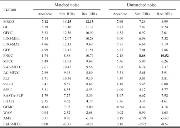
as multi-resolution cochleagram. Although Table 1 showed that Gammatone-based features are preferred over the others in terms of short-time objective intelligibility (STOI), it should be noted that the conclusion is only considered accurate on fully-connected DNN for IRM estimation at a certain range of SNR levels, and is probably not applicable whenever there is a change in network architecture, output target, or any different testing conditions. It is also worth mentioning that, using less-engineered features like log-magnitude spectrogram performs reasonably well while requires much fewer computations compared to highly-engineered features, and it is also relatively easy to take advantage of parallel computing, leading to a fast implementation. In practice, plain features such as spectral magnitude have also gained interest among many researchers because they are easy to obtain and perform reasonably well.

Overall, the choice of feature-target set has a great variety, and usually depends on the network architectures. Fully-connected DNN was once the most popular option for many researchers in SE, and thus highly-engineered feature-target set was therefore preferred as it can be used to train the network effectively and usually performs better. However, thanks to recent progress on CNN in the field of CV, it has been shown that CNN with certain structures can work considerably well on plain feature-target set such as magnitude spectrogram or complex spectrogram.

1.1.2

Neural networks

Fully-connected DNN is the most basic and probably the most popular model adopted in SE. Typical use of fully-connected DNN for SE includes log-power spectrum esti-mation [59], IBM and IRM estiesti-mation [57], and CIRM estiesti-mation [58], etc. It consists of an input layer, hidden layers and an output layer. Rectified linear unit (ReLU) is most often employed among hidden layers to address the vanishing gradient problem, which refers to the observation that the absolute value of gradient becomes smaller

Table 1: STOI improvements (in %) for a list of features averaged on a set of test noises. Sim. RIR represents simulated room impulse responses and Rec. RIRs

progressively during back-propagation, thus resulting in a poor training as the param-eters of lower layers being not modified effectively. The structure of the output layer, in particular, can be modified in many ways if the output is a combination of differ-ent targets. For example, Fig. 1 shows a fully-connected DNN for CIRM estimation, whose output layer consists of 2 sub-networks which use their own local connections to produce spectral masks for real and imaginary components, respectively.

Figure 1: A DNN for CIRM estimation [58]

Unlike fully-connected DNN, the structure of CNN is highly customizable which results in a great variety of design. A number of CNN structures have been explored for SE tasks, including SE-WaveNet [41], dilated residual CNN for mask estimation [50], and redundant convolutional auto-encoder [35], etc. The classic structure of CNN takes 2D images (3D if channel counts as one dimension) as input and performs

feature extraction by stacking pairs of a convolutional layer and a pooling (down-sampling) layer, and appending a couple of fully-convolutional layers at the end to obtain the output of any desired shape. The CNN of this structure could be simply employed in frequency-domain as spectrogram are of 2 dimensions just like images. In [8], a CNN with a similar structure is employed for SE task via complex spectro-gram estimation. Yet in many recent works, the pooling layers are often discarded or replaced by using stride and dilation with convolution, because it is argued that the pooling operation may be too destructive if the objective is to reduce the spatial size. Furthermore, researchers have proposed to replace fully-connected layers in the classic structure by 1d convolutional layers to obtain a fully convolutional network (FCN). Long et al. demonstrated that FCN can efficiently learn to perform per-pixel-prediction tasks such as semantic segmentation. Park and Lee proposed a FCN with autoencoder-decoder architecture for SE task via magnitude spectrogram-mapping and demonstrated that a CNN with a proper network structure could yield a com-parable SE performance as fully-connected DNN and RNN while being significantly more compact than both networks, as illustrated in Fig. 3.

Rethage et al. employed WaveNet [51] for SE task, which features a heavy use of dilated 1d convolution with skip-connection and residual learning. As is shown in Fig. 4, the network is fully convolutional, and in particular, the filters are all designed to be 1-dimensional. While 1d convolution is an efficient way to process time-domain speech, adopting plain 1d convolution may not be ideal as the network would fail to be trained effectively due to its limited receptive field. Specifically, the time-domain speech consists of dense and highly-correlated data due to the high sampling rate (e.g., the number of samples reaches 16k per second with a sampling rate 16kHz), yet stacking regular 1d convolution simply leads to a linear growth of the receptive field, which makes it impossible for CNN to capture the contextual information and perform feature extraction. The problem can be addressed by incorporating dilation within

(a) a CNN with fully-connected layers

(b) a fully convolutional neural network

Figure 2: Replacing fully-connected layers with 1×1 convolutional layers for semantic segmentation task [54]. The numbers denote the spatial size of feature maps in both (a) and (b).

cascading convolutional layers, which allows the receptive field to grow exponentially. We will give a more detailed introduction about CNN of this type in Chapter 2.

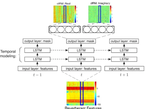
RNN, especially LSTM, has been studied for speech enhancement task for its ability of modeling temporal relations. The use of RNN is similar to that of fully-connected DNN in SE, thus a fully-fully-connected DNN could be simply replaced by a RNN without major modifications. While fully-connected DNNs are mostly designed to work in frequency-domain and the input usually contains a number of frames to consider the contextual information between the previous and current data, RNN, in contrast, only requires the single-frame input because it can model the contextual relation between two consecutive frames of the input. As an example, Fig. 5 shows a LSTM for CIRM estimation, where the only difference between this network and that in [58] is that the fully-connected DNN is replaced by LSTM and the input only consists of one frame. It is noteworthy that, while it is reasonable to use fewer units among the hidden layers of LSTM than that of fully-connected DNN, this does not mean the size of the model for LSTM is anywhere smaller than that of fully-connected

Figure 3: A comparison of SE performance of different network structures and their model size [35]. The FNN denotes fully-connected DNN.

Figure 4: Wavenet for SE

DNN since LSTM uses multiple sets of weights and biases to model the contextual information while the fully-connected DNN only uses one.

Generative models

While the deterministic models described above have been proven suitable for SE and are more straightforward than generative models in the context of SE task, generative models such as variational auto-encoder (VAE) and generative adversarial network (GAN) have also been investigated. It is claimed that, even though the deterministic model for SE adopts a supervised approach which already requires a fairly large

Figure 5: LSTM for CIRM estimation

amount of training data, it is still not very robust against unknown environments as it is not always possible to cover all noisy scenarios in real-world applications during training. [4].

A generative model usually does not make assumptions on the environmental noise, because it is often trained to generate clean speech, which means unsupervised training is employed and the training data only contains clean speech. For exam-ple, in [4], a VAE is employed as a generative model that is capable of generating the spectrogram of clean speech. In the context of SE, the model is adapted in a statistical approach to obtain clean speech from the noisy one. As shown in Fig. 6, the noisy speech is used as observed data to create a posterior distribution which the spectrogram of clean speech can be sampled from. The posterior distribution aims to minimize the semantic loss between the generated clean speech and the noisy speech. GAN, as a generative model, could be employed in a similar manner. However, it should be mentioned that, while GAN has been studied for SE tasks in a number of works, it is always adopted in a deterministic manner with supervised training, i.e.,

Figure 6: The VAE-based SE method [4]. X, N and S refer to the spectrograms of noisy speech, noise and clean speech, respectively, Z represents the latent variable sampled from the standard Gaussian prior, W denotes the spectral basis vectors and

H denotes the activation vectors, both of which are used to represent the spectrogram of noise.

the GAN is employed for explicit spectrum mapping, which is essentially the same as a deterministic model. We suggest that a similar approach as [60], which is designed for image inpainting in the field of CV, be adopted in the context of SE. Illustrated in Fig. 7, the input latent vector of GAN is updated iteratively to minimize the contextual loss between the masked image and the output image of GAN. To adapt the method, the spectrogram of noisy speech could be transformed into a masked spectrogram by energy-thresholding, and a specific loss function of noisy and clean spectrograms should be designed and minimized to find the best match to the spectrogram of the clean speech given the masked noisy one.

1.2

Training datasets and training strategy

The bias-variance tradeoff [10] is a long standing problem in machine learning which has to be considered when deploying deep-learning models for real-world applications. It could be illustrated by a typical observation that, the better the model fits the training data, the less likely that it will generalize well on unseen data, or vise versa. Specifically, a model trained with high-variance learning method would be able to represent the training data well, which unfortunately may lead to overfitting and

Figure 7: A GAN for image inpainting designed by a generative approach [60]. y is the masked input image and M denotes the mask. The output is the corresponding inpainted image. Left: The latent vectorzis updated iteratively based on a designed loss function to find the closest mapping to the masked image. Right: The output image manifold changes as z gets updated.

could produce poor results on unpresented data. In contrast, although the model trained with high bias does not overfit the training data, which consequently yields a simpler model, it may underfit the presented data and fails to capture some important regularities.

This bias-variance problem causes a series of problems when applying deep learn-ing models for SE. Typically, it makes the evaluation of different algorithms rather unreliable, because the results often fluctuate depending on the training and testing data as well as the metrics adopted. A common practice is to compare the model with some other methods of its kind with a specific dataset, yet the comparison is questionable even if all methods are trained on the same dataset, because it is usually uncertain if the testing data is in favor of high-variance model or high-bias model. For example, a high-variance model may easily outperform high-bias models on testing data that is similar to training set, yet outperformed by same high-bias models on testing data that is relatively unseen in training dataset.

evaluated with metrics covering different aspects. For example, high-biased models may be preferable to high-variance methods for ASR metrics, while the later may be more useful for general intelligibility metrics such as PESQ as indicated in [6].

While using a large and diverse training dataset does not directly resolve the dilemma, it is still considered very helpful for the evaluation of a model, and is particularly vital for deploying a model for real-world applications. The benefits of using a large dataset for training is straightforward: for high-variance models, it provides more instances, which hopefully covers more unseen cases where the high-variance model fails to work, and for high-bias models, it simply helps ease the training process as some important regularities may become obvious as more data is provided. The training dataset for SE usually consists of two parts: speech dataset and noise dataset.

1.2.1

Speech dataset

While a number of speech datasets could be used for SE tasks, in particular, the ones originally designed for ASR are preferred over the others because of their size and diversity. The characteristics concerning the speech dataset could be divided into two aspects: audio characteristics and text characteristics. Audio characteristics include the total duration of speech, the number of speakers and the distribution of speakers’ gender and age group, speech quality, dialect and accent, tempos of speech, etc. Text characteristics refer to the language of speech and the richness of language such as the number of words, etc. For SE task, important characteristics include the duration of speech, the number of speakers and the distribution of speakers’ gender, speech quality and the language of speech. Below, we briefly introduce some speech datasets that are considered as suitable for training SE models:

1) TIMIT [9]: TIMIT is often used in SE tasks for both training and evaluation purposes. It consists of 6300 utterances from 192 female speakers and 438 male

speakers, each speaking 10 short annotated sentences. With a total duration of approximately 5 hours, it also features 8 major dialect divisions of American English.

2) TED-LIUM [18, 44, 45]: TED-LIUM is a public domain speech dataset that contains hundreds of hours of TED [2] talks in English language. The first version [44] consists of a total duration of 188 hours of talks, which come from 666 speakers (about 70 percent of the audio are from male speakers) with a mean duration of 9 minutes per talk. The second [45] and third versions [18] continue to enrich the dataset as more TED talks are added. Designed for the training of ASR systems, it is fairly rich in terms of languages, with 2.56m

words covered in talks. The audio is accompanied with automatically aligned transcripts, which is also useful for identifying the speech segments. As the talks were previously recorded in conference halls that were full of audiences, the audio is noticeably reverberant and noisy (with the appearance of sound such as cough and applause).

3) LibriSpeech [34]: LibriSpeech is an archive of public domain English audiobooks from LibriVox [1]. It contains about 1k hours of speech that is sampled at 16 kHz. The speech comes from approximately 2.5kspeakers, and about 52 percent of the speakers are male. The mean duration is limited to 25 minutes to avoid major imbalances in per-speaker audio duration.

4) MUSAN [47]: As its name suggests, music, speech and noise corpus (MUSAN) is a complementary dataset that comprises audios of music, speech and noise. As described in the original paper, this dataset is suitable for training models for voice activity detection (VAD) and music/speech discrimination. The speech portion of the dataset contains about 60 hours of speech, with about 20 hours of multi-language speech from LibriVox and 40 hours of collected recordings from

US government (federal and states) hearings, committees and debates. About half of the LibriVox audios are in English and the rest is in 11 other languages. The recordings of US government hearings are completely in English.

1.2.2

Noise dataset

Noise dataset is a collection of recordings of different soundscapes. Ideally, it should contain a wide range of sound types to minimize the gap between training and real-world applications. While there exist certain datasets initially designed for training and evaluating SE models, many of them only provide recordings of non-stationary noise whose types are rather limited. Another major drawback is that plenty of them are not in public domain and thus often require licensing, making it hard for researchers to obtain. For example, a commonly-used dataset in SE is NOISEX-92 [53], which provides 5 types of noise: voice noise (babble), factory noise, HF radio channel noise such as pink noise and white noise, military noises including fighter jets (Buccaneer, F16), destroyer noises (engine room, operations room), tank noise (Leopard, M109) and machine gun, and lastly, car noise (Volvo). Though it may be suitable for the initial evaluation, the dataset lacks a variety of soundscapes in daily life, thus it does not meet the demand of most real-world scenarios.

Realizing the fact that, depending on the context, noise could literally be any kind of sound, a more convenient way is to utilize datasets that are originally designed for tasks such as sound event detection where a wide range of sound is presented. As an example, ESC-50 dataset [37] contains 50 types of labeled recordings which could be loosely divided into 5 major categorizes that are shown in Table 2. The dataset has a total duration of around 2 hours and the mean duration of each type of sound is approximately 2.4 minutes.

Table 2: The types of sound in ESC-50 dataset Animals Natural soundscapes & water sounds Human, non-speech sounds Interior, domestic sounds Exterior, urban noises

Dog Rain Crying baby Door knock Helicopter

Rooster Sea waves Sneezing Mouse click Chainsaw

Pig Crackling fire Clapping Keyboard typing Siren

Cow Crickets Breathing Door, wood

creaks

Car horn

Frog Chirping birds Coughing Can opening Engine

Cat Water drops Footsteps Washing machine Train

Hen Wind Laughing Vacuum cleaner Church bells

Insects (flying) Pouring water Brushing teeth Clock alarm Airplane

Sheep Toilet flush Snoring Clock tick Fireworks

Crow Thunderstorm Drinking, sipping Glass breaking Hand saw

1.2.3

Training strategy

The training strategy generally depends on the specific deep-learning models. For SE task, it is often straightforward to adopt supervised training as the task can be categorized into sequence regression [39]. A deterministic neural network model is designed as a unique mapping function from features to certain target and is trained with a loss function that is usually defined using the mean-square distance or`1-norm between the true value of the target and its prediction. Most existing methods are designed in this deterministic manner and usually yield a promising performance. The training targets are sometimes preprocessed and transformed, e.g., the DNN-based CIRM adopts hyperbolic tangent transform to compress its range of values from (−∞,∞) to (−1,1).

Though not being the mainstream, unsupervised, or semi-supervised training could also be applied on certain generative models such as variational auto-encoder (VAE) and generative adversarial network (GAN). The model is often trained on clean speech dataset in order to model the speech with its probability distribution. For example, in [4], a VAE is adopted along with non-negative matrix factorization

(NMF) and is trained on clean speech in advance and then adapted to noise on the fly. It is claimed to outperform conventional DNN-based methods in unseen noisy environments.

While there are barely any so-called best practices for training the neural networks for SE tasks because the training process varies on different models and usually re-quires a lot of experiments and tweaking of the network and related parameters, a few practices are commonly considered appropriate in order to make the neural net-work models suitable for real-world applications. For example, the speech data used for training should be gender-balanced covering all age groups, and the duration of speech per speaker should be unified. The noise data used in training should be representative and cover common scenarios like urban soundscapes. On the other hand, RMSprop [13] and Adam [21] optimizers are often applicable for training neu-ral network models for SE task. RMSprop uses the average of the magnitude of the recent gradients whileAdam considers the moments of the gradients. Both optimizers provide a more stable training over classic stochastic gradient descent (SGD).

1.3

SE Objective and evaluation

While the overall task of speech enhancement is to improve the speech quality in noisy speech environments, specific application scenarios such as mobile communication, hearing aids and automatic speech recognition (ASR) may have different concerns on the objectives and performance metrics. For example, for hearing air and mobile communication, improving the intelligibility of speech is a main goal, while on ASR the main focus is to reduce the word error rate (WER) to improve the noise-robustness of the system.

It should be noted that the performance of a SE system on certain objectives and metrics does not necessarily relate to the performance on the others. For example,

even if a SE system yields improvement on intelligibility, WER is not necessarily guaranteed to be improved. Empirically optimization for WER is a more challenging task than improving intelligibility as the ASR system sometimes serves as a black box, yet it is believed that a joint optimization between ASR and SE system is required in order to avoid the sub-optimization problem that could lead to an unstable performance of the system.

1.3.1

Evaluation of intelligibility

Most commonly-used metrics for the evaluation of speech intelligibility could be di-vided into perception-level and signal-level [55]. Perception-level metrics include per-ceptual evaluation of speech quality (PESQ) [42] and short-time objective intelligibil-ity (STOI) [20, 49]. PESQ is a standard metric which predicts the perceptual mean opinion score (MOS) of a given speech in a interval of −0.5 to 4.5. The auditory transform is applied on both reference clean speech and the speech to be measured to obtain their corresponding loudness spectrograms. MOS is then predicted by compar-ing the two loudness spectrograms. On the other hand, STOI reflects the short-time intelligibility in a range of 0 to 1, and it is achieved by measuring the correlation between the short-time temporal envelopes of the reference speech and the speech to be evaluated. Although STOI has been reported to tend to over-predict the intelli-gibility scores [17, 24], it is still considered accurate as it consistently correlates with human intelligibility.

Signal-level metrics quantify the degree of distortion with respect to clean refer-ence at the signal level. Popular metrics comprise signal-to-distortion ratio (SDR) and segmental signal to noise ratio (SSNR). It is noticeable that, while PESQ and STOI model subjective intelligibility test scores which directly reflect the level of intelligibility, the results on SDR and SSNR are usually consistent with PESQ and STOI, as the more clean the speech is, the more intelligible to human ears.

1.3.2

Evaluation of ASR performance

For the evaluation of ASR performance, the metrics are WER for large vocabulary continuous speech recognition (LVCSR) systems, and false reject rate (FRR) and false alarm rate (FAR) for keyword spotting (KWS) systems. It should be noted that, as multi-style training (MTR) has been employed in state-of-the-art ASR systems and effectively improves the noise robustness [6, 26], a SE system that serves as pre-processor may still be beneficial. However, it has been shown that adopting a SE model for this purpose requires retraining the MTR model with both noisy and enhanced features, otherwise it may degrade the ASR performance compared to the ASR without any enhancement [6].

1.4

Objective and organization of this thesis

1.4.1

Objective of the thesis

The main objective of this thesis is to develop single-channel speech enhancement methods with deep neural networks for noise reduction.

In the first approach, a fully convolutional network is proposed for complex spec-trogram estimation in speech enhancement. The network adapts the WaveNet frame-work [51] for 2-dimensional spectrogram processing. Stacked frequency-dilated convo-lution is employed to obtain an exponential growth of the receptive field in frequency domain, which enables an efficient implementation that requires much fewer parame-ters as compared with conventional fully-connected DNN and CNN while still yielding a comparable performance.

Although speech enhancement is useful in noisy conditions, it is often redundant for clean speech. As most voice activity detection (VAD) techniques that are adopted as pre-processor in SE methods are not designed to identify the SNR levels, conven-tional SE methods usually do not adapt to different noisy conditions. In the second

contribution, we proposed a model that considers different SNR levels and provides an automatic ”on/off” switch for speech enhancement. It is capable of scaling its com-putational complexity under different SNR levels by detecting clean or near-clean speech which requires no processing. By adopting information maximizing generative adversarial network (InfoGAN) in a deterministic, supervised manner, we incorporate the functionality of SNR-indicator into the model that adds little additional cost to the system.

1.4.2

Organization of the thesis

The rest of this thesis is organized as follows:

Chapter 2: This chapter first introduces complex spectrogram processing in speech enhancement and some network structures that are suitable for this task, including fully-connected DNNs and CNNs. It then gives detailed description of the proposed fully convolutional network for complex spectrogram estimation. Comparative study of the proposed method with other existing methods is also presented.

Chapter 3: This chapter describes the generative adversarial network and its application in speech enhancement. It introduces the information maximizing generative adversarial network (InfoGAN) and the proposed InfoGAN-based SE method. Experimental results of the proposed approach and related methods are given on the aspects of speech intelligibility and KWS.

Chapter 4: This chapter concludes this thesis and gives some directions for future research.

Chapter 2

Single-Channel Speech

Enhancement with Convolutional

Network

In this chapter, we develop a method for single-channel speech enhancement using convolutional neural network. This chapter is organized as follows. In this section, we introduce background and recent works in CNN-based speech enhancement methods. Section 2.2 describes the proposed CNN model for single-channel speech enhancement. Performance of the proposed CNN method is evaluated in Section 2.3.

2.1

Previous work

2.1.1

Complex spectrogram processing by DNN

Conventional deep-learning-based SE methods process speech signal in frequency do-main, where the main focus is to obtain the spectral magnitude of clean speech. Given a noisy speech y, a common practice is to first apply short-time Fourier transform (STFT) to the signal: Y = STFT(y), where Y refers to as the spectrogram and

is a matrix with size of K ×L, with K representing the number of time segments and L the number of frequency bins. While Y takes natural complex-valued, i.e.,

Y = Yr +Yi where Yr represents the real STFT component and Yi the imaginary

STFT component, the spectral magnitude is simply |Y|, the absolute value of Y, and phase is defined asφy =arctan(Yi/Yr). The spectral magnitude of clean speech,|X|,

is then estimated as |Xˆ|with a neural network and transformed back to time domain along with the spectral phase of noisy speech by using inverse short-time Fourier transform (iSTFT): ˆx= iSTFT[|Xˆ|ejφy_{]. A number of methods have been developed}

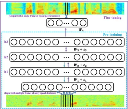
in this manner. To name a few, the DNN-based log-power spectrum estimation [59], the DNN-based ideal ratio mask [57], the CNN-based spectrogram estimation [35]. For example, the DNN-based log-power spectrum estimation [59] employs a fully-connected DNN to estimate the log-power spectrogram (LPS) of clean speech given that of noisy speech as shown in Fig. 8. The detailed block diagram of the corre-sponding SE system is shown in Fig. 9. Specifically, the time-domain noisy speech is first transformed into frequency domain by computing the discrete Fourier trans-form (DFT) of each overlapping windowed frames, the result of which is often called spectrogram. The logarithm of the squared value of the spectrogram is calculated to obtain the log-power spectrogram, which is then fed into the neural network as input. The output of neural network is transformed back into spectral magnitude of the estimated clean speech, which, along with the spectral phase of noisy speech, is used to synthesize the estimated clean speech in time domain.

It should be noted that, while there are some methods that directly process speech signal in time domain [36, 41] which yields an end-to-end solution, most of the ex-isting algorithms are designed to work in frequency domain given the fact that it’s relatively fast (time-domain convolution equals element-wise multiplication in fre-quency domain) and the harmonic structure of clean speech is disentangled from the mixture in frequency domain.

Figure 8: A DNN for LPS estimation. The DNN contains three hidden layers with 2048 units per hidden layer. The input of DNN consists of several consecutive frames of LPS of noisy speech and the output is a single frame of LPS of estimated clean speech [59].

As described, most of the spectral-based speech enhancement algorithms only modify the magnitude of the STFT components and leave the phase untouched, because it is generally considered that the magnitude carries most of the information of a signal. Yet recent studies have shown that employing spectral phase can further improve the perceptual quality of speech [11, 23, 33]. Specifically, Krawczyk and Gerkmann [23] showed that the perceptual evaluation of speech quality (PESQ) could be improved by around 0.2 when using the combination of noisy magnitude and estimated phase for speech reconstruction. While it may be beneficial to process noisy phase for a better denoising performance, it remains difficult to directly estimate the true phase of clean speech from noisy phase using deep learning, possibly due to the wrapping effect and the lack of phase structure in human speech [8, 58].

Figure 9: The block diagram of DNN for LPS estimation. Y denotes noisy speech and X denotes clean speech [59].

[36, 41], where the spectral magnitude and phase are jointly processed in an implicit way. However, models of this kind are often outperformed by frequency-domain-based methods, possibly because the structure of speech in time domain may be overwhelm-ing for neural network to capture, which, on the other hand, is greatly disentangled in frequency domain in view of the harmonic structure of spectral magnitude of speech. Another possible walk-around of phase processing is through complex spectrogram estimation. As shown in Fig. 10, Williamson et al. [58] found that the structure of complex spectrogram is similar to that of magnitude spectrogram, which makes it feasible to simply reuse a neural network that is originally designed for spectral magnitude estimation for estimation, while maintaining another neural network for

magnitude processing.

A few speech enhancement methods have been developed based on the esti-mation of complex noisy spectrogram, in which the noisy phase is implicitly pro-cessed. Williamson et al. [58] proposed a DNN-based masking technique to estimate a complex-valued mask from a spectral feature set by employing a fully-connected DNN, where the hidden layers of the fully-connected DNN are shared, and both real and imaginary components of the complex mask are simultaneously estimated by the output layers of the DNN. The resultant model is reported to improve the SE per-formance as compared with the fully-connected DNN employed for ideal ratio mask (IRM) estimation.

On the other hand, Fu et al. [8] employed a CNN to estimate the complex spectro-gram of clean speech directly from the noisy one. As shown in Fig. 11, the structure of CNN consists of both convolutional layers and fully-connected layers. Though both methods are reported to have achieved a better denosing performance compared with DNN-based magnitude-processing methods, no further evidence is given to show the effectiveness of phase estimation through complex spectrogram processing.

2.1.2

Convolutional neural networks for speech enhancement

Fully-connected deep neural network remains as the most common choice for speech enhancement tasks and is often adopted as a non-linear mapping function between noisy features and clean ones [32, 57–59]. Researchers have attempted to replace the fully-connected DNN by other neural network models, among which CNN has gained increasing popularity thanks to the recent progress in the filed of CV.

CNNs are known to be highly customizable and flexible in terms of the network design. Various network structures have been introduced and investigated for SE task. A classic CNN structure shown in Fig. 11 is employed in [8]. This conventional design

(a) A speech signal in time-domain

(b) Spectral magnitude (c) Spectral phase

(d) Real STFT component (e) Imaginary STFT component

features a joint use of convolutional layers and fully-connected layers (sometimes calleddense layers). Intuitively, convolutional layers could be considered as a feature extractor which produces some high-dimensional features. These features are then fed into the fully-connected layers that map the noisy features of speech to some targets that are latter used to reconstruct the clean speech.

Park and Lee [35] proposed a fully convolutional network (FCN) for speech denos-ing, where CNN is employed to extract the features for the reconstruction of the clean speech. The proposed CNN is a variant of the encoder-decoder network named Re-dundant Convolutional Encoder-Decoder network (R-CED) as shown in Fig. 12. The classic encoder-decoder design shown in Fig. 13 is a popular CNN structure that is often adopted as the structure of generator in generative adversarial network (GAN). Ideally, the encoder compresses the input into some high-dimensional features and the decoder reconstructs the data based on the high-level features. The spatial size of feature maps often shrinks (which refer to downsampling) among the encoder lay-ers to compress the input to some latent representation, and then expands among the decoder layers (upsampling) to reconstruct the data, and meanwhile, the number of feature maps increases within the encoder and decreases within the decoder. As opposed to this, the R-CED uses a different way to produce the high-level represen-tation and reconstruct data. Assuming the high-dimensional represenrepresen-tation of the input can be provided by enough feature maps, downsampling is abandoned among the encoder layers, and it is replaced by increasing the number of channels of filters. Consequently, upsampling is replaced by decreasing the number of channels within the decoder layers.

It should be mentioned that, although both classic CNN with dense layers and fully convolutional network (FCN) could be considered as the non-linear mapping function in SE task, FCNs are often more restricted as they require the input feature and output target to have the same form (e.g., both to be magnitude spectrogram).

The conventional CNNs that consist of fully-connected layers, on the other hand, usually do not have this problem. The possible reason is that, the receptive field of fully-connected layers is generally larger than that of convolutional layers due to their difference in connectivity. The convolutional layers use a local connectivity that is limited by the size of the filters, while the fully-connected layers use a full connectivity (as suggested by its name), which, on the other hand, often leads to a greater number of parameters to model this connection.

Figure 11: A CNN for complex spectrogram estimation [8]

2.1.3

WaveNet framework

WaveNet [51] is a generative convolutional model designed for audio synthesis and is proposed by DeepMind, Google. As shown in Fig. 14, dilated 1d convolution is stacked by many layers and the dilation is increased by a factor of 2, which allows for an exponential expansion of the receptive field. For example, as illustrated in Fig. 14, stacking 4 dilated 1d convolutional layers with filter size of 2 can produce a receptive field with a size of 16. In practice, the dilation factor is doubled for every layer up to

Figure 12: The network sturcture of redundant convolutional encoder-decoder (RCED) [35]

Figure 13: A FCN with autoencoder-decoder design [35]

512 and then repeated, e.g., 1, 2, 4, .., 256, 512, 1, 2, 4, .., 256, 512, 1, 2, 4, ..., 256, 512.

In order to fit the context of autoregressive audio generation, the CNN models the joint conditional probability of the waveform x:

p(x) =

T

Y

t=1

p(xt|x1, ..., xt−1) (5)

where xt represents the audio sample at time step t, which is conditioned on the

samples at all previous time steps. Naturally, the convolution must obey the causality, as the model cannot violate the sequence of prediction: the audio sample xt cannot

convolution and implemented by shifting the output of a normal convolution in time domain.

Figure 14: Stacked dilated causal 1d convolution [51]. Solid lines refer to the current dilated causal convolution and the dashed lines refer to the past and future convolu-tion.

Fig. 15 further illustrates its network architecture, which features a gated activa-tion funcactiva-tion [52]:

z= tanh(Wf,k∗x)σ(Wg,k∗x) (6)

whereW denotes the convolution filter, k indexes the layer, f represents filter and g

represents gate, ∗ and represent convolution operation and element-wise multipli-cation, respectively, and σ(˙) is the sigmoid function.

As shown in the figure, the network stacks a number of convolution layers which consists of the basic components: dilated convolution, gated activation function and 1×1 convolution. The residual learning and skip connection are used across different layers, which further take advantage of the efficient 1×1 convolution to perform the channel mapping.

The WaveNet has been successfully applied to SE [41]. As illustrated in Fig. 4, the SE WaveNet keeps the same processing block while employing the non-causal, dilated 1d convolution, which essentially change the functionality of the network from the sequential, non-parallelizable time-domain audio sample prediction to parallizable regression. As shown in Fig. 16, the input to SE WaveNet consists of previous samples

Figure 15: The network structure of WaveNet [51]

and future samples. While the SE task does not require causality, it introduces some latency as future samples are a part of the input. Though the result does not compare with modern deep-learning-based models, it is reported to outperform traditional Wiener filtering method.

2.2

Proposed fully convolutional neural network

for speech enhancement

2.2.1

Dilated 2-d and 1-d frequency convolution

The input to the CNN consists of a limited number of successive spectrogram frames. However, the frequency dimension is usually several hundreds and requires a larger size of receptive field in order to exploit the contextual information. Thus, as a common practice, it is necessary to increase the size of the filters in the frequency dimension, e.g., Fu et al. [8] used a filter with size of 25 in frequency in their imple-mentation.

As discussed before, dilated convolution has been applied in various contexts in-cluding imaging segmentation [61] and speech synthesis [51]. In dilated convolution, whenever a filter weight is applied to the input, a fixed number of input values are skipped, which makes the size of receptive field larger than that of the filter. Stack-ing dilation convolution results in an exponential expansion of the receptive field. In WaveNet, dilation is heavily employed to capture the signal in time domain with massive samples, however, for frequency-domain CNN, the actually input is often a context window of a spectrogram that contains several frames in order to consider the time-domain contextual information, and each frame is a vector that usually consists of a few hundred frequency bins. Since the dimension of frequency is significantly larger than that of time, dilation is only needed at frequency axis to incorporate the frequency information. Hence, we introduced frequency-dilated 2-d convolution, which is shown in Fig. 17

By stacking this dilated convolution with an increasing dilation factor, one could keep the size of filter relatively small, while obtaining a large receptive field in fre-quency. For example, stacking 7 layers of such a frequency-dilated convolution with a filter size of 3 and dilation of 1, 2, 4, 8, 16, 32, 64 will enlarge the receptive field

Figure 17: Frequency dilated 2-d convolution

correspondingly, with its size being 3, 7, 15, 31, 63, 127, 255 for each layer. Naturally, using a large filter with dilation of this kind can increase the size of receptive field even more rapidly, for example, when the filter size is increased to 17, stacking 4 layers will eventually produce a receptive field of size 241.

On the other hand, the proposed network also adopts 1-d convolution, which is a special case where the filter is only of 1-dimension. In Fig. 18, the 1-d convolution is applied along frequency axis. It is more efficient than 2-d convolution when the goal is to increase the size of receptive field along frequency axis only. Hence it has been used in some recent works [35, 50]. A special type of 1-d convolution is 1_×1 convolution, where the filter size is simply 1×1. Although it does not increase the size of the receptive field, it has been commonly used for channel adjustment, because of its small kernel size which is highly efficient.

2.2.2

Network architecture

Inspired by WaveNet [51], here we propose a convolutional network for complex spec-trogram estimation as shown in Fig. 19. It is fully convolutional and consists of a set of 2-d convolutional layers (denoted as Conv2d) and 1-d convolutional layers (Conv1d). The Conv2d layer uses both frequency-dilated 2-d convolution and regular

Figure 18: 2d convolution an 1d convolution

1-d convolution, while the Conv1d layer only uses regular 1-d convolution along the frequency axis. It is possible to combine real and imaginary spectrograms as the input [8], yet we find treating them separately may lead to a better performance.

Figure 19: The network structure of the proposed CNN

The input to the CNN consists of 13 frames. Stacking Conv2d layers allows the receptive field of time to increase linearly. When the size of the receptive field along time axis equals or exceeds the number of input frames, the central frame of the output of Conv2d layers will contain the information from all input frames. Hence it

is extracted as the input to Conv1d layers to produce a single-frame output.

Table 3 shows a configuration of the proposed CNN. The Conv2d layers are stacked 6 times with frequency dilation increased by a factor of 2 (i.e., 1, 2, 4, 8, 16, 32), which yields a receptive field of size 253 in frequency and size 13 in time. The Conv1d layers are stacked 2 times, followed by the output layer, which is simply 1-d convolution for different channels (denoted as 1d-real and 1d-imag in the table) to separately produce the real-valued frame and the imaginary-valued frame.

Similar to the WaveNet, in our proposed network, the Conv2d layers also adopt a residual learning and skip-connection structure [15, 51] to ease the training of a deeper network. The residual path provides the next Conv2d layer with lower dimen-sional data from the previous layer which may be destructively compressed during the convolution process [35], while the skip connection provides the Conv1d layer with the data processed at the current Conv2d layer.

Table 3: The Network Configuration (Config.1). The height of the filter is the size along the frequency axis, and the width is the size along the time axis. The channel refers to the depth, or the number of feature maps of convolution.

Layer name Filter name Height Width Channel dilated 2d 5 3 48 Conv2d 1d-skip 1 1 48 1d-residual 1 1 48 Conv1d 1d 3 1 96 Output 1d-real 3 1 1 1d-imag 3 1 1

2.3

Performance evaluation

2.3.1

Performance measure of speech quality

To evaluate the performance of the proposed model in terms of speech intelligibility, we conducted experiments using TIMIT database [9], in which 780 utterances from both female and male speakers are used for the training and 90 utterances used for testing. Four typical non-stationary noises (babble, street, factory and restaurant) are randomly truncated and used for both training and testing stages. The sampling rate is set to 16 kHz. The SNR levels for training and testing stages are set to -5 dB, 0 dB, 5 dB and 10 dB. We evaluate the proposed CNN towards two aspects: speech quality, and the model complexity.

Comparison with previous models

The proposed CNN is compared with two other complex-spectrogram processing methods: CIRM [58] and RI-CNN [8]. As introduced before, CIRM is a DNN-based method that estimates a complex mask from a set of spectral features. RI-CNN is a CNN model that consists of convolution layers and fully-connected layers, and takes complex spectrogram as input.

For a fair comparison, all networks are trained and tested with the database and the SNR level described above. All models use 500-point DFT with 50% overlap. Apart from the DFT length, both reference methods are implemented with the con-figuration described in the original papers, which makes the number of parameters for RI-CNN, CIRM and the proposed CNN to be 775K, 3.87M and 243K, respectively. Aforementioned SSNR and PESQ are used as performance metrics. Table 4 shows the result obtained from each network. Clearly, the proposed CNN outperforms RI-CNN, while achieving a comparable performance to CIRM but with around 16 times fewer

of parameters (243K parameters of proposed CNN compared with 3.87M parameters of CIRM).

Table 4: PESQ and SSNR score of different models

metrics PESQ SSNR SNR -5 dB 0 dB 5 dB 10 dB -5 dB 0 dB 5 dB 10 dB unprocessed 1.337 1.678 2.043 2.403 −12.627−8.901 −4.373 0.274 CIRM 1.824 2.279 2.649 2.956 −1.137 1.332 3.914 5.959 RI-CNN 1.760 2.115 2.421 2.616 −3.094 −0.584 1.601 3.409 proposed 1.951 2.349 2.672 2.972 −1.786 1.255 4.301 7.052

Benefit to phase processing

To further investigate whether complex spectrogram processing is beneficial to phase estimation, we combine the clean magnitude with either noisy phase or estimated phase from estimated complex spectrogram to synthesize the speech. We have com-pared the proposed CNN with the two other complex-spectrogram processing meth-ods. The average PESQ scores for both female and male speech are shown in Fig. 20.

Figure 20: Average PESQ score on female and male speech by replacing phase of noisy speech with that of estimated clean speech.

Again, the proposed method shows a comparable performance with CIRM. RI-CNN is found to be the least effective in phase processing with complex spectrogram estimation. For female speech, a maximal improvement of 0.15 is observed. Yet for male speech, the improvement is less significant, possibly indicating that the perceptual quality of female speech is more prone to phase distortion than that of male, and thus benefited more from phase processing.

It is worth mentioning that, in terms of phase processing, current complex spec-trogram estimation algorithms may be less effective than algorithms like [23], which only and directly estimates phase of clean speech and could improve the PESQ score by merely using the estimated phase with the spectral magnitude of noisy speech for reconstructing the estimated clean speech. For complex spectrogram estimation algorithms, however, when using the combination of noisy magnitude and estimated phase from the processed complex spectrogram, the improvement on PESQ is rather limited.

Performance measure with restricted model complexity

Some recent works that utilize CNN for speech processing have considered a situation where the number of parameters is limited [35, 46]. Thus in the third experiment, we have configured the model in a parameter-controlled manner. In addition, the memory footprint of the proposed CNN is also considered. While it is rather im-plementation dependent, a rough measure could be (size of spectrogram)×(2d con-volution channel)×(1d convolution channel of Conv2d layers)×(size of float). Two configurations of the proposed CNN with parameters at the level of 100K and 50K

are tested for the overall denoising performance.

By stacking 6 Conv2d layers and 2 Conv1d layers, the configuration shown in Table 3 has 243K parameters, and the memory footprint is around 29 megabytes (MB). Meanwhile, two configurations shown in Table 5 and Table 6 keep the number

Table 5: A network configuration where the number of parameters is 97K (Config.2) Layer name Filter name Height Width Channel

dilated 2d 5 3 32 Conv2d 1d-skip 1 1 24 1d-residual 1 1 24 Conv1d 1d 5 1 64 Output 1d-real 17 1 1 1d-imag 17 1 1

Table 6: A network configuration where the number of parameters is 50K (Config.3) Layer name Filter name Height Width Channel

dilated 2d 5 3 32 Conv2d 1d-skip 1 1 16 1d-residual 1 1 16 Conv1d 1d 1 1 48 Output 1d-real 17 1 1 1d-imag 17 1 1

of Conv2d and Conv1d layers unchanged, but use fewer filter channels to reduce the number of parameters and the memory footprint at the same time. The config.2 shown in Table 5 has 97K parameters, and the memory footprint is 10 MB. The config.3 in Table 6 further reduces the parameters and the memory footprint to 50K and 6 MB, respectively. Figure 21 illustrates the overall performance for all three configurations. While the model with 97K parameters still produces a good overall result, the one with 50K suffers more loss on PESQ score. Generally speaking, config.2 seems to reach a good balance between the denosing performance and memory efficiency.

2.3.2

Performance measure of keyword spotting

An application of speech enhancement is to improve the performance of speech recog-nition system under noisy conditions. In this case the speech enhancement method

Figure 21: Performance comparison with different model configurations could be considered as a pre-processor. It has been reported that the traditional objective of speech enhancement may not be consistent with the objective of speech recognition, i.e., a better speech quality doesn’t necessarily result in a better speech recognition performance. Empirically, SSNR is preferred over PESQ if no prior knowl-edge of the speech recognition algorithm is obtained.

To evaluate whether the proposed CNN is applicable for SE for speech recognition, we use a keyword spotting engine that detects keywordAlexa. The engine is assumed to be a black-box, i.e., no prior knowledge is given except that it will output a stream of boolean decision wheretrue indicates a keyword has been detected andfalse

otherwise. We use two metrics for the evaluation, namely false-reject rate (FRR) and false-alarm rate (FAR). FRR refers to the number of keywords being ignored by the engine given a stream of keyword and FAR refers to the number of occurrences that the engine detects a keyword when the input is some other sound. In addition, we train the same model on various datasets and demonstrate that the choice of training dataset can be crucial as stated in Chapter 1.