Abstract: Handoff failure probability in cellular systems is
defined as the probability that a handoff request is denied for lack of resources, and premature call termination probability is defined as the probability that an accepted ongoing call is terminated due to lack of recourses, are two of the main parameters used to study and analyze several cellular system performance measures. Further, they are the main parameters that are used in quality of service studies and teletraffic analysis of such a network during the planning and development stages. To evaluate the handoff failure probability, premature call termination probability, and other system performance measures such as call dropping probability, several statistical distributions have been used in the literature to model the channel holding time distribution in 3rd and 4th generations cellular systems, such as exponential, Erlang, Gamma, and generalized Gamma, hence, the complexity of the analytical and simulation models introduced in literature varies based on the assumed channel holding time distribution in addition to other assumed parameters. In this paper the effect of the statistical distribution used to model the channel holding time on handoff failure probability and premature call termination probability are investigated using analytical and simulation models, where the main goal of the research is to determine the level of complexity of the statistical distribution used to model the channel holding time to accurately evaluate the handoff failure probability and premature call termination probability.
Index Terms: cellular system, handoff failure probability,
premature call termination
I. INTRODUCTION
ECENT advance in wireless communications and cellular systems make it possible for cellular networks to support a wide variety of services to the user on the move. 4G systems and future wireless networks enable the user to make voice, data, multimedia calls, or make an internet connection to surf the web, and retrieve data. These advance services have motivated the study of network's quality-of-service (QoS), in cellular networks. The following QoS measures are the most important measures used to specify the quality of the services:
New call blocking probability ܲ: defined as the
probability that a new call request be denied for lack of resources.
Manuscript received July 13, 2011; revised July 30, 2011. This work was supported by the Deanship of Research at University of Tabuk, Saudi Arabia.
Mohammed M. Alwakeel is with the college of Computers and Information Technology at University of Tabuk, Saudi Arabia, Tabuk, P. O. Box 741 (email: [email protected]).
Premature call termination probability ܲ௧: defined as
the probability that an accepted on going call is terminated due to lack of recourses.
Call dropping probability ܲௗ: defined as the
probability that a call will experience either premature call termination or new call blocking.
Handoff failure probability ܲ : defined as the
probability that a handoff request is denied for lack of resources.
Some of these measures may be specified in the design, for example, in second generation cellular systems, the premature call termination probability is lower than 5%, and the handoff failure probability is lower than 2% for voice calls [1]. Many previous literature introduced techniques and expressions to evaluate handoff failure probability, premature call termination probability, number of handoff probability and handoff rate. In early literature the following assumptions are commonly used: the call holding time, the cell residence time, and the channel holding time are assumed to be exponentially distributed, and calls arrival is a Poisson process [2,3,4,5]. However, because of technological advances and the growing interest in personal communication services, and because of new marketing service plans (e.g. flat-rate service), mobile users behavior pattern was changed such that they use their mobile devices for longer period of time and more frequently. Hence, the exponential distribution may no longer appropriately models the service time or the interarrival time of practical 3G and 4G networks [6,7,8,9]. In recent literature, several techniques were introduced to determine number of handoff probability and handoff failure probability where more general call holding time, cell residence time, and channel holding time distributions were assumed [1,10,11], hence, based on the used distributions the complexity of the introduced analytical and simulation models varies. In this paper the effect of the statistical distribution used to model the channel holding time on handoff failure probability and premature call termination probability is investigated using analytical and simulation models, where the main goal of the research is to determine the level of complexity of the statistical distribution used to model the channel holding time to accurately evaluate the handoff failure probability and premature call termination probability. The rest of this paper is organized as follow: In section 2, an analytical model to evaluate handoff failure probability and premature call termination probability is investigated. In section 3, the simulation model used to validate the analytical results is introduced. In section 4, the results and discussion are presented, and finally the conclusion is in section 5.
The Effect of Channel Holding Time
Distribution on Handoff Failure Probability and
Call Termination Probability
Mohammed M. Alwakeel
II. THE ANALYTICAL MODEL The cellular system considered is presumed to have N channels in each cell, of which S channels are reserved for handoff only and the remaining
N S
channels are used to serve both new calls and handed-off calls. The assumed system is connection-oriented. Once a channel is assigned to a particular user, that channel cannot be used by any other user until the channel is released either when the call is completed or when the user moves to another cell. Whenever a new call arrives at an arbitrary cell (origination cell), if there is a free channel (out of theN S
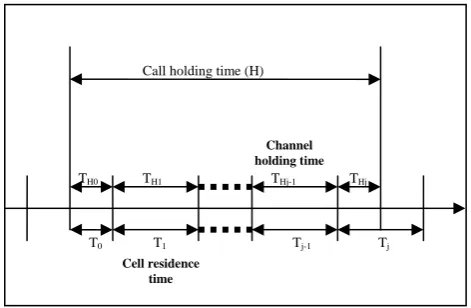
channels) available to support the call, the call will be accepted and remains in that cell until it is completed or handed-off to next cell. On the other hand, if there is no channel available to support the newly arrived call, it will be blocked. Whenever there is a handoff request, the call will be handed-off to the next cell if there is a free channel in the next cell to accept the handed-off call; otherwise, the call will be dropped. Based on this scenario, one can consider the system under modeling as a birth and death process in which blocked calls are cleared (no queue) [12]. To determine expression for Phf, one must clearly understand thedefinitions of the call holding time, the channel holding time, and the cell residence time that are illustrated in Fig. 1. The call holding time is defined as the period from the instant the accepted call starts to the instant the call completes. The channel holding time is defined as the period from the instant an active call occupies the channel to the instant the active call releases the channel. The cell residence time in the origination cell is defined as the time that the mobile user travels from the point where the call originated to the edge of the cell. In any subsequent cell, the residence time is defined as the time that the mobile user travels through the cell (edge to edge).
[image:2.595.50.286.474.628.2]
Fig. 1. Timing diagram for a call ended at j-th cell
From the above definitions, it can be concluded that the service time for any particular call in any cell is the channel holding time. The channel holding time is found as min(RHi,Ti), i = 0,1,…, where Ti is the residence time in a
cell that is reached after i handoff, and RHi is the remainder
of the call holding time at the time when the call enters the cell. In the origination cell, we have min(RHi,Ti) =
min(H,T0), where H is the call holding time, as shown in
Fig. 1. In order to simplify the analysis, in deriving analytical expression in this research for Phf it is assume that
the call interarrival time follows a negative exponential distribution (which is usually the case in real world) [12], [13-15]. The scenario presented in this Section suggests that there are two call arrival processes in the system under study namely, new call arrival process and handoff call arrival process. Note that the active calls in any cell may be divided into two groups. The first group includes calls that will end in that cell itself so that such calls from this group will not affect the handoff call arrival process to next cell.
The second group includes calls that travel through the cell and will issue a handoff request to next cell when they reach the edge of the current cell; hence, the calls in this group represent the handoff arrival to next cell. For a call from the second group, the channel holding time in the current cell may be found as min(RHi,Ti) = Ti (the cell
residence time). Based on this, one may conclude that the arrival process of handoff calls depends on the distribution of the cell residence time. Therefore, in order to evaluate Phf
we need to verify that for the assumed cell residence time model, the distribution of the interarrival time of handoff calls may be approximated accurately by the negative exponential distribution. In fact, the assumption that the distribution of the interarrival time of calls in PCS systems can be approximated accurately by a negative exponential distribution, even though the channel holding time and the cell residence time have distributions other than exponential, agrees with the results obtained from empirical data collected from working PCS systems and presented in [14], [16].
A. Basic Assumptions
In the present analysis, the following commonly used assumptions are assumed: New call arrival is a Poisson process with average arrival rate n, [12-16]. The handoff
call arrival may be accurately approximated by a Poisson process with average arrival rate h, [12]. The number of
channels per cell is N. The number of channels per cell reserved for handoff is S. At equilibrium, all cells have a similar behavior. The users are uniformly distributed in each cell. The call duration H is a random variable with finite mean with probability density function denoted by fH(t). The
cell residence time in the first cell is modeled by a random variable T0, and the cell residence times in all other cells are
modeled by a random variable Ti. The cell residence times
are independent, and the cell residence times in all cells where calls are handed-off (Ti) are identical.
B. Determination of Handoff Failure Probability (ܲ)
The number of channels reserved for handoff would affect the handoff failure probability. In general, there are two main scenarios that may be used in cellular system: (i) No handoff priority scenario and (ii) prioritized handoff scenario. In the following, the procedure to determine Phf in
these scenarios is discussed.
i. No Handoff Priority Scenario
Assume that the average channel holding time in a cell is
, the new call arrival rate isn, and the handoff arrival rate
is h. Consequently, the mean of the overall arrival process
(new calls and handed-off calls) can be found as n h
[12], [14]. Since a blocked-calls-cleared approach is followed in the present system, it is possible to model call-handling events in the system as a birth andCall holding time (H)
T0 T1 Tj-1 Tj
TH0 TH1 THj-1 THj
Cell residence time
death process as long as the channel holding time has a finite mean [13]. If no channel is reserved for handoff (i.e.
0
S
), then the handoff failure probability Phf may befound as
0
!
!
N
n h
hf N k
n h
k
N
P
k
(1)
ii. Prioritized Handoff Scenario
Consider a cell with guard channels reserved for handoff (i.e.
S
0
). Since handed-off calls have higher priority than new calls, then they will be cleared from the system if there is no idle channel available in the cell, whereas new calls will be cleared from the system if there are less than1
S
idle channels. Then, handoff failure occurs when there are N busy channels, which can be written as( ) ( )
*
(
)
(
)
!
N S S
n h h
hf
P
P
N
(2)where is the average channel holding time, and P* is defined as
1
* ( )
0 1
( ) ( )
( )
! !
k k S N
N S N
N S
h n h
h n
k k N S
P
k k
(3)To evaluate Phf using , (1) and (2) we need first to
determine the average channel holding time and the average handoff arrival rate h. This is done in the following
subsections.
C. Determination of Average Channel Holding Time () The cell residence time model, as mentioned earlier, comprises two components. The first is the residence time in the origination cell, modeled by the random variable T0. The
second is the residence time in subsequent cells where calls are handed-off, modeled by the random variable Ti (
1, 2,3,...
i
). From the above definitions, the channel holding time in the first cell (TH0), may be determined as thesmaller of the call duration and the residence time in that cell [3], [14]. The channel holding time in a subsequent cell i (
i
1, 2, 3,...
), where a call is handed-off, (THi) is eitherthe cell residence time if the remaining call holding time is longer than the cell residence time, or the remaining call holding time if the call will be completed in that cell. The cdf of the channel holding time in the first cell can be derived as
H0 0
T = min (H,T )
. (4)Then
Pr
0
1 Pr
0
Ho
T H H
F
t
T
t
T
t
.Since TH0 is greater than t if and only if H > t and T0 > t,
then
1 Pr
,
0
Ho
T
F
t
H
t T
t
. (5)Since H and T0 are independent, then
1 Pr
Pr
0
Ho
T
F
t
H
t
T
t
(6)and
1
1
1
0
Ho
T H T
F
t
F
t
F
t
. (7) Therefore,
0
( )
( )
( ) 1
( )
H o
T H T H
F
t
F t
F t
F t
. (8)From (8), the pdf of the channel holding time in the first cell can be expressed as
0( ) ( ) ( ) ( ) ( ) 1 ( )
H o o
T H T H T H
f t f t F t f t f t F t , (9)
where
0
( ), ( )
0T T
f
t
F
t
fH(t), and FH(t) are the pdf of theorigination cell residence time, the cdf of the origination cell residence time, the pdf of the call holding time, and the cdf of the call holding time, respectively. After passing the first cell, the remaining average call holding time may be found as
E H
E T
0 . Based on the assumptions, the average number of cells a handed-off call will pass through until the call is completed, if the call does not drop due to handoff failure, is [17]
i 0E H
E T
M
E T
, (10)where
x
is the "CEIL" function which returns the smallest integer greater than or equal to x,E T
0 is theaverage cell residence time in origination cell,
E H
is the mean call duration, andE T
i , (i=1,2,…) is the mean of residence time in subsequent cells where calls are handed off, with
1
2...
i1, 2,...
E T
E T
E T
i
. (11)Therefore, the average channel holding time in any cell other than the origination cell
E T
Hi may be found as
0Hi
E H
E T
E T
M
. (12)The average channel holding time is obtained as a weighted combination of the average channel holding time in the first cell and the average channel holding time in subsequent cells, and the weight of each component is given by [12]
1
1
1
1
n n
n n h hf
P
K
P
P
, (13)
2
1
1
1
h hf
n n h hf
P
K
P
P
. (14)From (12), (13), and (14), the average channel holding time is obtained as [12]
1 H0
+
2 HiK E T
K E T
, (15)where
E T
H0 may be found from (9) as 0
0 0 0
( ) ( ) ( ) ( ) 1 ( )
o o
H H T H T H
E T tf t dt tF t f t dt t f t F t dt
. (16)D. Determination of Average Handoff Arrival Rate (
h)The determination of the average arrival rate of handed-off calls h is greatly simplified if the call duration and/or
The memoryless property implies that the remaining time of a call has the same distribution as its duration [12]. For a call duration distribution that does not possess the memoryless property, the determination of the average arrival rate of handoff calls is more complicated. One may start by assuming that for a stationary observer in a particular cell, ongoing calls (on average) experienced l successful handoffs before reaching that cell, where
1
2
M
l
, (17)and M is given in (10). At equilibrium, h can then be
determined from [12]
0 1
(1 ) Pr( ) (1 )
h n Pn H T h Phf pl
, (18)
where
h(1
P
hf)
p
l1 represents the number of calls handed-off successfully to cell l-1 that has call holding time long enough to reach the edge of that cell and request a handoff to cell l, andp
l1 is defined as
11
2
la l
p
a l
, (19)where
a j
is given by
Pr
j
0,1,.., -1, ,....a j HG j l l (20)
and 0 1 0
1, 2,...
0.
j i i jT
T
j
G
T
j
(21)Solving (18) for h, we have
0
1
(1
) Pr(
)
1 (1
)
n n
h
hf l
P
H
T
P
p
. (22)As a special case, when H follows the exponential distribution,
p
l1 does not depend on l; and since it is assumed that T1, T2,.., Tl-1 are i.i.d. random variables, (20)can be written as
0 1
0 1
0
0 0 1
Pr ...
Pr
Pr ...
Pr Pr ...
j
j
H T T T H T T
a j H T
H T H T T T
. (23) Then, using the memoryless property of the exponential distribution, (23) becomes
Pr
0
Pr
1
j
a j
H
T
H
T
. (24)From (24), it is observed that
1 11
2
la l
p
P H
T
a l
. (25)Note that, substituting (25) in (22) agrees with [12]. However, when H has a distribution that does not possess the memoryless property, the evaluation of h using (22)
requires the knowledge of the pdf of
G
j, which will be discussed in the next section.Note that Pn, Phf, , and h are interdependent. Therefore,
an iterative technique must be used to evaluate them. One may start by assuming initial (estimated) values for Pn and
Phf, and calculate and h using equations (15) and (22),
respectively. The calculated values of and h are then used
as inputs to equation (2) , to update the value of Phf. These
steps are repeated until the values of Phf converge.
E. Approximating the pdf of Gj
Let
j
G
f
t
denote the pdf of the random variableG
j. The determination of
j
G
f
t
requires j-fold convolution and, to the best of our knowledge, analytically it is not known exactly. An approximation of
j
G
f
t
may be found using central limit theorem. However, since Gj is the sum ofnon-negative random variables, one may apply a causal form of the central limit theorem. This is based on the fact that the Gaussian approximation for
j
G
f
t
asj
will not yield a causal distribution no matter how large the mean of Gj. It is appropriate, therefore, that for sufficientlylarge j,
j
G
f
t
may be approximated by a two parameters gamma distribution
1
/( )
j j
j j
z t b
G z
j j
t
e
f
t
u t
b
z
, (26)where
10
x t
x
t
e dt
is the gamma function and theparameters
z
j andb
j are given by
0
2 2
0
2 2 2 1, 2,....
j T Ti
j i
j
G
E G E T jE T
z i j
(27)
and
0
2 2 2 0 1, 2,... T T j i G j i j j b i
E T jE T
E G , (28)
where 2
j
G
is the variance of Gj, 02
T
is the variance of T0,and 2
i
T
is the variance of Ti.F. Determination of Premature Call Termination Probability (Pct)
One should understand that Phf and Pct are not the same;
while Phf is the probability that an arbitrary handoff request
is denied, "Pct has a long-term flavor denoting the
probability that a call will be terminated at some point during its life time", hence, premature call termination probability may be determined once the handoff failure probability are evaluated. The definition of probabilities Pct
may be found as:
0
1
Pr( ) 1
j
ct hf hf hf
j
P H T P P P a j
(29)was concluded from the analysis that was presented in this section.
III. SIMULATION MODEL
The developed simulation model is an event-driven model that is highly modular and flexible. The arrival of new call event is activated based on the inputs and the assumptions of the simulation. The following actions may result when the arrival of new call occurs:
Block the call and clear it if no channel is available to carry the new call
Assign a channel to the call if there is an available channel
Generate the call holding time based on the assumed distribution
Generate the residence time in the first cell only
Increment the counter for new calls
Increment the counter for new blocked calls if the new call blocked and cleared.
The arrival of handoff call event will be activated when the remaining residence time of any call in any cell is zero. The following actions may result when the arrival of handoff call occurs:
Remove the call from the current cell and free the used channel
Assign a new channel in the next cell to carry the call if a free channel is available in the next cell
Drop the call if there is no free channel available in the next cell
Generate the cell residence time in the next cell where call is handed-off
Increment the counter for handoff requests
Increment the counter for handoff failure if the call is dropped.
The call completion and removal events are activated when the remaining call holding time of any call is zero. The following actions may result when the call completion and removal occur:
Remove the call from the system and free the channel used in the current cell
Increment the counter of successfully completed calls
The impact of various parameters of the cellular system on the performance can be easily investigated, including the number of channels in each cell, the arrival rate of new calls, the arrival rate of handed-off calls, the distribution of call duration, and the cell residence time. The functions used in the simulation may be classified into two groups. The first group includes the functions that scan the occurrence of the events and accordingly schedules the next event. The second group includes the function that performs the actions that result when an event occurs.
IV. RESULTS AND DISCUSSION
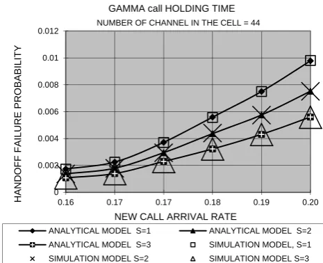
As we mention earlier the type of the statistical distribution of the channel holding time has no impact on handoff failure probability or premature call termination
[image:5.595.314.547.214.403.2]probability, and by sing the analytical model and the simulation model presented in section 2 and 3 respectively, Fig. 2 and 34 show that the analytical results and the simulation result are in a great agreement, where, in Fig. 2 the handoff failure probability is presented as a function of new call arrival rate. From the figure we can see that as the new call arrival rate increases the handoff failure probability increases due to lack of available channel. In Fig. 3, the premature call termination probability is show as a function of new call arrival rate, and the premature call termination probability shows the same behavior as the handoff failure probability in both analytic a simulation model, which can be seen directly from (29).
[image:5.595.309.542.439.621.2]Fig. 2. Handoff failure prob. vs. new call arrival rate
Fig. 3. Premature call termination Prob. vs. new call arrival rate
V. CONCLUSION
In this paper we investigate the impact of the type of the statistical distributions used to model channel holding time in cellular system on handoff failure probability and premature call termination probability. The analytical model investigated in this research shows that the type of the channel holding time distribution has no impact on the handoff failure probability and premature call termination probability. Instead, the mean of the channel holding time which is a constant value that depends on the parameters of the system such as the design layout and users distribution
0 0.002 0.004 0.006 0.008 0.01 0.012
0.16 0.17 0.17 0.18 0.19 0.20
HANDOFF FAILURE
PROBABILITY
NEW CALL ARRIVAL RATE
ANALYTICAL MODEL S=1 ANALYTICAL MODEL S=2 ANALYTICAL MODEL S=3 SIMULATION MODEL, S=1 SIMULATION MODEL S=2 SIMULATION MODEL S=3
GAMMA call HOLDING TIME
NUMBER OF CHANNEL IN THE CELL = 44
0 0.005 0.01 0.015 0.02 0.025 0.03 0.035 0.04 0.045 0.05
0.16 0.17 0.17 0.18 0.19 0.20
PR
EM
AT
U
R
E
C
ALL T
ER
M
IN
AT
ION
PR
OBABILIT
Y
NEW CALL ARRIVAL RATE
ANALYTICAL MODEL S=1 ANALYTICAL MODEL S=2 ANALYTICAL MODEL S=3 SIMULATION MODEL S=1 SIMULATION MODEL S=2 SIMULATION MODEL S-3
GAMMA HOLDING TIME
in the service area, regardless of the type of distribution used to model the channel holding time, has direct impact on the handoff failure probability and premature call termination probability. The result obtained from the analytical model is validated using simulation. Base on the results, the research recommends that to study the performance of a cellular system the researchers may use any statistical distribution to model the channel holding time as long as it leads to simplifying the developed model and produce a close form solution. However, the values of the parameters of the distribution used in the analysis or the simulation must be selected very carefully such that the moments of the used distribution reflect the moments of the practical system (usually the first three moments are enough).
REFERENCES
[1] Y. Fang, "Modeling and performance analysis for wireless mobile networks: A new analytical approach", IEEE/ACM Trans. on
Networking, Vol. 13, No. 5, Oct. 2005, pp. 989-1002.
[2] R. A. Guerin, "Channel occupancy time distribution in a cellular radio system", IEEE Trans. Veh. Technol., vol. 35, no. 3, Mar. 1987, pp. 89–99.
[3] D. E. Everitt, "Traffic engineering of the radio interface for cellular mobile networks", Proc. IEEE, vol. 82, no. 9, Sep. 1994, pp. 1371– 1382.
[4] T.-S. P. Yum and K. L. Yeung, "Blocking and handoff performance analysis of directed retry in cellular mobile systems", IEEE Trans. Veh. Technol., vol. 44, no. 3, Jun. 1995, pp. 645–650.
[5] D. Hong and S. S. Rappaport, "Traffic model and performance analysis for cellular mobile radio telephone systems with prioritized and nonprioritized handoff procedures", IEEE Trans. Veh. Technol., vol. VT-34, no. 3, 1986, pp. 77–92.
[6] M. Rajaratnam and F. Takawira, "Nonclassical traffic modeling and performance analysis of cellular mobile networks with and without channel reservation", IEEE Trans. Veh. Technol., vol. 49, no. 3, May 2000, pp. 817–834.
[7] C. Jedrzycki and V. C. M. Leung, "Probability distributions of channel holding time in cellular telephony systems", Proc. IEEE Vehicular
Technology Conf., Atlanta, GA, May 1996, pp. 247–251.
[8] J. Jordan and F. Barcelo, "Statistical modeling of channel occupancy in trunked PAMR systems", Proc. 15th Int. Teletraffic Conf., 1997, pp. 1169–1178.
[9] V. A. Bolotin, "Modeling call holding time distributions for CCS network design and performance analysis", IEEE J. Sel. Areas
Commun., vol. 12, no. 3, Mar. 1994, pp. 433–438.
[10] Z. Yan and S. Boon-Hee, "Handoff counting in hierarchical cellular system with overflow scheme", Computer Networks journal, Vol. 46, 2004, pp. 541-554.
[11] R. Rodriguez-Dagnino and H. Takagi, "Counting handovers in a cellular mobile communication network: equilibrium renewal process approach", Performance Evaluation Journal, No. 52, April 2003, pp. 153-174.
[12] G. Ruiz, L. Doumi, and G. Gardiner, "Teletraffic analysis and simulation for nongeostationary mobile satellite systems", IEEE
Transactions on Vehicular Technology, vol. 47, pp. 311 -320,
February 1998.
[13] A. Zaim, H. Perros, and G. Rouskas, "Computing call-blocking probabilities in LEO satellite constellations", IEEE Transactions on
Vehicular Technology, vol. 52, pp. 622-636, May 2003.
[14] P. Fitzpatrick, M. Ivanovich, and J. Yin, "Models for pre-emption of packet data by voice in slotted cellular radio networks", Proceedings
of IEEE Global Telecommunications Conference, vol. 2, pp.
1698-1702, November 2002.
[15] K. Yeo and C. Jun, "Teletraffic analysis of cellular communication systems with general mobility based on hyper-Erlang characterization", Journal of Computer and Industrial Engineering, vol. 42, pp. 507-520, 2002.
[16] C. Jedrzycki and V. Leung, "Probability distribution of channel holding time in cellular telephony systems", Proceeding of IEEE