NeuroRule: A Connectionist Approach to Data Mining

(1)

NeuroRule:

A Connectionist

Approach

to Data Mining

Hongjun Lu

Rudy Setiono

Huan Liu

Department

of Information

Systems Computer

Science

National University

of Singa.pore

{luhj,rudys,liuh}@iscs.nus.sg

Abstract

Classification, which involves finding rules that partition a given da.ta set into disjoint groups, is one class of data mining problems. Approaches proposed so far for mining classification rules for large databases are mainly decision tree based symbolic learning methods. The connectionist approach based on neura.l networks has been thought not well suited for data mining. One of the major reasons cited is that knowledge generated by neural networks is not explicitly represented in the form of rules suitable for verification or inter- pretation by humans. This paper examines this issue. With our newly developed algorithms, rules which are similar to, or more concise than those generated by the symbolic methods can be extracted from the neural networks. The data mining process using neural networks with the emphasis on rule extraction is described. ExperimenM results and comparison with previously published works are presented.

1 Introduction

With the wide use of advanced database technology developed during past deca.des, it is not difficult to ef- ficiently store huge volume of data in computers a.nd retrieve them whenever needed. Although the stored Permission to copy without fee all or part of this material ir granted provided that the copies are not made or distributed for

direct commercial advantage, the VLDB copyright notice and the title of the publication and its date appear, and notice is given that copying is by permission of the Very Large Data Base Endoc1rmen.t. To copy otherwise, or to republish, requires a fee and/or special permission from the Endowment.

Proceedings of the Zlst VLDB Conference

Ziirich, Switzerland, 1995

data are a valuable asset of a.n organization, most orga- nizations may face the problem of data rich but knowledge poor sooner or later. This situation aroused the recent surge of research interests in the area of data mining [l, 9, 21.

One of the data mining problems is classification.

Data items in databases, such as tuples in relational database systems usually represent real world entit,ies. The values of the attributes of a tuple represent the prqperties of the entity. Classification is the process of finding the common properties among different entit#ies and classifying them into classes. The results a,re often expressed in the form of rules - the classification rules. By applying the rules, entities represented by tuples can be easily classified into different classes they belong to. We can restate the problem formally defined by hgrawal et al. [l] as follows. Let A be a set, of attributes Al, AZ,. . . , A,

and dom(Ai) refer to the set of possible values for attribute Ai. Let C be a set of classes cl, ~2, . . . , cm. We are given a data set, the training set whose members are (n+ 1)-tuples of the form (al, as,. . . , a,, ck) where

ai E dom(Ai),(l 5 i < n) and ck E C(l 5 k 5 m).

Hence, the class to which each tuple in the training set belongs is known for supervised learning. We are also given a second large database of (n. + I)-t$uples, the testing set. The classification problem is to obtain a set of rules R using the given training data set. By applying these rules to the testing set, the rules can be checked whether they generalize well (measured by the predictive accuracy). The rules that generalize well can be safely applied to the application database with unknown classes to determine each tuple’s class.

This problem has been widely studied by researchers in the A.1 field [28]. It is recently re- examined by database researchers in the context of large database systems [5,7, 14, 15, 131. Two basic approaches to the classification problems studied by AI researchers are the symbolic approach and the connectionist approach. The symbolic approach is based on decision trees and the connectionist approach mainly

(2)

uses neural networks. In general, neural networks give a lower classification error rate than the decision trees but require longer learning time [17, 24, 181. While both approaches have been well received by the AI community, the general impression among the database community is that the connectionist approach is not well suited for data mining. The major criticisms include the following:

1. Neural networks learn the classification rules by multiple pssses over the training data set so that the learning time, or the training time needed for a neural network to obtain high classification accuracy is usually long.

2. A neural network is usually a layered graph with t#he output of one node feeding into one or many other nodes in the next layer. The classification rules are buried in both the structure of the graph a,nd the weights assigned to the links between the nodes. Articulating the classification rules becomes a difficult problem.

3. For the same reason, available domain knowledge is rather difficult to be incorporated to a neural network.

Among the above three major disadvantages of the connectionist approach, the articulating problem is the most urgent one to be solved for applying the tech- nique to data mining. Without explicit representation of classification rules, it is very difficult to verify or interpret them. More importantly, with explicit rules, tuples of a certain pattern can be easily retrieved using a database query language. Access methods such as indexing can be used or built for efficient retrieval as those rules usually involve only a small set of attributes. This is especially important for applications involving a large volume of data.

In this paper, we present the results of our study on a.pplying the neural networks to mine classification rules for large databases with the focus on articulating the classification rules represented by neural networks. The contributions of our study include the following:

l Different from previous research work that ex-

cludes the connectionist approach entirely, we ar- gue that, the connectionist approach should have its position in data mining because of its merits such as low classification error rates and robust- ness to noise [17, 181.

l With our newly developed algorithms, explicit

classification rules can be extracted from a neural network. The rules extracted usually have a lower classification error rate than those generated by the decision tree based methods. For a data set

with a strong relationship among attributes, the rules extracted are generally more concise.

l A data mining system, NeuroRule, based on neu-

ral networks was developed. The system success- fully solved a number of classification problems in the literature.

To better suit large database applications, we also developed algorithms for input data pre-processing and for fast neural network training to reduce the time needed to learn the classification rules [22, 191. Lim- ited by space, those algorithms are not presented in this paper.

The remainder of the paper is organized as follows. Section 2 gives a discussion on using the connectionist approach to learn classification rules. Section 3 describes our algorithms to extract classification rules from a neural netswork. Section 4 presents some experimental results obtained and a comparison with previously published results. Finally a conclusion is given in Section 5.

2 Mining

classification

rules using neu-

ral networks

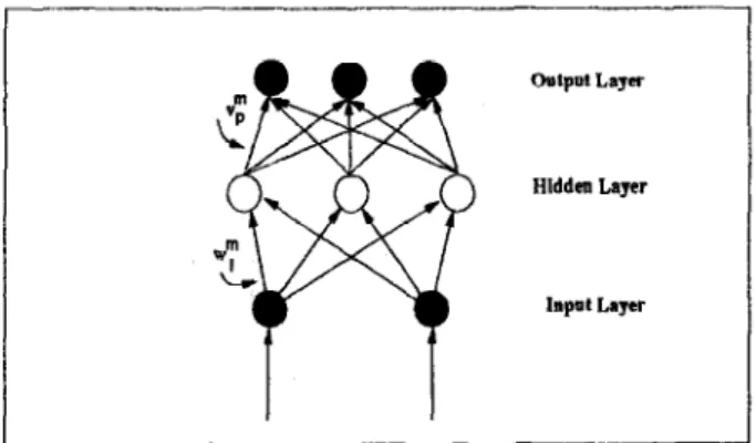
Artificial neural networks are densely interconnected networks of simple computational elements, neurons. There exist many different network topologies [lo]. Among them, the multi-layer perceptron is especially useful for implementing a classification function. Fig- ure 1 shows a three layer feedforward network. It consists of an input layer, a hidden layer and an output layer. A node (neuron) in the network has a number of inputs and a single output. For example, neuron Hj has x:,x;, . . . ,z: as its input and ,j as its output. A link in the network is associate! with a weight. The input links of Hj has weights til, u$, . . .,&i. A node computes its output, the activation value by summing up its weighted inputs, subtracting a threshold, and passing the result to a non-linear function f, the activation function. Outputs from neurons in one layer are fed as inputs to neurons in the next layer. In this manner, when an input tuple is applied to the input layer, an output tuple is obtained at the output layer. For a well trained network which represents the classification function, if tuple (x1,22,. . . , 2,) is applied to the input layer of the network, the output tuple,

(Cl,%*-., cm) should be obtained where ci has value

1 if the input tuple belongs to class ci and 0 otherwise. Our approach that uses neural networks to mine classification rules consists of three steps:

1. Network tmining

A three layer neural network is trained in this step. The training phase aims to find the best set

(3)

of weights for the network which allow the network to classify input tuples with a satisfactory level of accuracy. An initial set of weights are chosen randomly in the interval [-l,l]. Updating these weights is normally done by using informa- tions involving the gradient of an error function. This phase is terminated when the norm of the gradient of the error function falls below a pre- specified value.

2. Network pruning

The network obtained from the training phase is fully connected and could have too many links and sometimes too many nodes as well. It is impossi- ble to extract concise rules which are meaningful to users and can be used to form data.base queries from such a network. The pruning phase aims at removing redundant links and nodes without increasing the classification error rate of the network. A smaller number of nodea and links left in the network after pruning provide for extracting consise and comprehensible rules that describe the classification function.

3. Rule extraction

This phase extracts the classification rules from the pruned network. The rules generated are in the form of “if (alhl) and (c#va) and . . . and (z,&) then Ci” where ai’s are the attributes of an input tuple, vi’s are constants, 0’s are re lational operators (=, <,>, <>), and Cj is one of the class labels. It is expected that the rules are concise enough for human verification and are easily applicable to large databases.

In this section, we will briefly discuss the first two phase. The third phase, rule extraction phase will be discussed in the next section.

2.1 Network training

Assume that input tuples in an n-dimensional space are to be classified into three disjoint classes d, f?, and C. We construct a network a9 shown in Figure 1 which consists of three layers. The number of nodes in the input layer corresponds to the dimensionality of the input tuples. The number of nodes in the output layer equals to the number of classes to be classified, which is three in this example. The network is trained with target values equal to { 1, 0, 0) for all, patterns in set

d,

(0, 1, 0) for all patterns in f?, and (0, 0, 1) for all tuples in C. An input tuples will be classified as a member of the class A, B or C if the largest activation value is obtained by the first, second or third output node, respectively.

There is still no clear cut rule to determine the number of hidden nodes to be included in the network. TOO

many hidden nodes may lead to overfitting of the data and poor generalization, while too few hidden nodes may not give rise to a network that learns the data. Two different approaches have been proposed to over- come the problem of determining the optimal number of hidden nodes required by a neural network to solve a given problem. The first approach.begins with a min- imal network and adds more hidden nodes only when they are needed to improve the learning capability of the network [3, 11, 191. The second approach begins with an oversized network and then prunes redundant hidden nodes and connections between the layers of the network. We adopt the second approach since we are interested in finding a network with a small number of hidden nodes as well as the least, number of input nodes. An input node with no connection to any of the hidden nodes after pruning plays no role in the butcome of classification process and hence can be removed from the network.

ChItput Lays

Hidden Layer

lapot Layer

Figure 1: A three layer feedforward neural network. The activation value of a node in the hidden layer is computed by passing the weighted sum of input values to a non-linear activation function. Let WY be the weights for the connections from input node e to hidden node m. Given an input pattern xi, i E {l,%..., k}, wherq iE is the number of tuples in the data set, the activation value of the m-th hidden node is

C-P

= f

(

k(x:w;1) -em ,

kl 1

where f(.) is an activation function. In our study, we use the hyperbolic tangent function

f(x) := d(x) = (es - ee5)/(ez + e+)

as the activation function for the hidden nodes, which makes the range of activation values of the hidden nodes [-1 , 11.

Once the activation values of all the hidden nodes have been computed, the p-th output of the network

(4)

for input tuple xi is comput#ed as

where vp” is the weight of the connection between hidden no& m and output node p a,nd h is the number of hidden nodes in the network. The activation function used here is the normal sigmoid function,

u(x) = l/(1 + e-“),

which yields activation values of the output nodes in the range [0, 11.

A tuple will be correctly classified if the following condition is satisfied

where $ = 0, except for iii = 1 if a? E A, ta = 1 if xi E a, and ti = I if xi E C, and 91 is a small positive number less than 0.5. The ultimate objective of t,he training phase is to obtain a set of weights that make the network classify the input t,uples correctly. To measure the classification error, an error function is needed so that the training process becomes a process to adjust the weights (w, V) to minimize this function. Furthermore, to facilitate the pruning phase, it is desired f,o .have many weights with very small values so that. they ca.n be set to zero. This is achieved by adding a penalty term to the error function.

In our training algorithm, the cross entropy function

qw, v) = - -& 2 (t; log% + (1 - tf, log(1 - $))

i=l o=l

(2)

is used as the error function. In this example, o equals to 3 since we have 3 different classes. The cross entropy function is chosen because faster convergence can be achieved by minimizing this function instead of the widely used sum of squared error function [26].

The penalty term P(w, V) we used is

/h n h o \

E-2

(c c MY2

+ c c tc)‘) )

m=l kl m=l p=l

where ~1 aad ~2 are two positive weight decay parameters. Their values reflect. the relative importance of the accuracy of the network versus its complexity. With larger values of these two parameters more weights

may be removed later from the network at the cost of a decrease in its accuracy.

The training phase starts with an initial set, of weights (ZU, U) (“) and iteratively updates the weights to minimize E(w, V) + P( UJ, v). Any unconstrained minimization algorithm ca,n be used for t,his purpose. In pa.rticular, the gradieut descent method has been the most. widely used in the training algorithm known as the backpropagation algorithm. A number of alterna- tive algorithms for neura.l network training have been proposed [4]. To reduce the network training time, which is very important in the data. mining as t,he data set is usually large, we employed a variant of the quasi- Newton algorithm [27], the BFGS method. This algorithm has a superlinear convergence rate, as opposed to the linear rate of the gradient descent method. De- tails of the BFGS algorithm can be found in [6, 231.

The network training is t,erminated when a local rninimum of the function E(ul, V) + P(w, V) has been reached, that is when the gradient of the function is sufficiently small.

2.2 Network pruning

A fully connected network is obta.ined at the end of the training process. There are usually a large number of links in the network., With n input nodes, h hidden nodes, a.nd m output, nodes, there are h(m + n) links. It is very difficult to articulate such a network. The network pruning phase aims at removing some of t,he links without affecting the classification accuracy of the network.

It can be shown that [20] if a network is fully trained to correctly classify an input tuple, xi, with the condition (1) satisfied we can set WY t,o zero without deteri- orating the overall accuracy of the network if t,he product IPwLPI issufficiently small. If maxp IzIyulrI 5 4712 and the sum (~1 + 772) is less than 0.5, then the network can still classify xi correctly. Similarly, if maxp Iup”\ 5 4q2, then up” can be removed from t,he network.

Our prunung algorithm based on this result is shown in Figure 2. The two conditions (4) and (5) for pruning depend on the magnitude of the weights for connections between input nodes and hidden nodes and between hidden nodes and output nodes. It is imperative that during training these weights be pre- vented from getting too large. At the same time, small weights should be encouraged to decay rapidly to zero. Ry using penalty funct,ion (3), we can achieve both. 2.3 An example

We have chosen to use a function described in [2] as an example to show how a neural network can be trained and pruned for solving a classification problem. The

(5)

Table 1: Attributes of the test da.ta adapted from Agrawal et a1.[2]

Mribute Description Value

salary salary uniformly distributed from 20,000 to 150,000 commission commission if salary 1 75000 -+ commission = 0

else uniformly distributed from 10000 to 75000. age age uniformly distributed from 20 to 80.

elevel education level uniformly distributed from 0 to 4. car make of the car uniformly distributed from 1 to 20.

xipcode zip code of the town uniformaly chosen form 9 available zipcodes.

hva.lue value of the house uniformaly distributed from 0.5klOOOO to 1.5k1000000 where Ic E (0 . . .9} depends on zipcode.

hyears years house owned uniformly distributed from 1 to 30. loan total amount of loan uniformly distributed from 1 to 500000.

input tuple consists of nine attributes defined in Ta- ble 1. Ten classification problems are given in [2]. Limited by space, we will present and discuss a few functions and the experimental results.

The original Function 2 classifies a tuple in Group A if

Neural network pruning algorithm (NP)

1. Let ~1 and 02 be positive scalars such that ~11 + 772 < 0.5.

2. Pick a fully connected network. Train this network until a. predetermined accuracy rate is achieved and for each correctly classified pattern the condition (1) is satisfied. Let (w,~) be the weights of this network.

3. For each WY, if

then remove ~7 from the network

4. For each v”‘, if

then remove up” from the network

5. If no weight satisfies condition (4) or condition G-9, th en remove WY with the smallest product maxp Iv,“’ x wy1.

6. Retrain the network. If accumcy of the network falls below an acceptable level, then stop. Other- wise, go t.0 Step 3.

Figure 2: Neural network pruning algorithm

((age < 40) A (50000 5 salary < 1000OO))V

((40 5 age < 60) A (75000 _< salary 5 125000))V

((age > 60) A (25000 5 salary _< 75000)). Otherwise, the tuple is classified in Group B.

The training data set consisted of 1000 tuples. The values of the attributes of each tuple were generated randomly according to the distributions given in Ta- ble 1. Following Agrawal et al. [2], we dso included a perturbation factor as one of the parameters of the random data generator. This perturbation factor was set at 5 percent. For each tnple, a class label was determined according to the rules that define the function above.

To facilitate the rule extraction in the later phase, the values of the numeric attributes were discrctized. Each of the six attributes with numeric values was discretized by dividing its range into subintervals. The attribute salary for example, which wits uniformly distributed from 25000 to I50000 was divided into 6 subintervals: subinterval 1 contained all salary values that were strictly less than 25000, subinterval 2 contained those greater than or equal to 25000 and strictly less than 50000, etc. The thermometer coding scheme was then employed to get the binary representations of these intervals for inputs to the neural network. Hence, a salary value less that 25000 was coded a~ {000001}, a salary value in the interval [25000,50000) was coded as {000011}, etc. The second attribute commission was similarly coded. The interval from 10000 to 75000 was divided into 7 subintervals, each having a width

(6)

of 10000 except for the last one, [~OOOO, 750001. Zero commission was coded by all zero values for the seven inputs. The coding scheme for the other attributes are given in Table 2.

Table 2: Binarization of the attribute values Attribute Input number Interval width

salary xl - 556 25000 commission z7 - 213 10000 w 214 - z19 10 elevel 220 - 223 car 124 - 143 zipcode 144 - 152 hvalue z-s3 - 166 100000 hyears 167 - x76 3 loan 277 - &36 50000

With this coding scheme, we had a total of 86 binary inputs. The 87th input was added to the network to incorporate the bias or threshold in each of the hidden node. The input value to this input was set to one. Therefore the input layer of the initial network consisted of 87 input nodes. Two nodes were used at the output layer. The target output of the network was { 1,O) if the tuple belonged to Group

A,

and (0, 1) otherwise. The number of the hidden nodes was initially set as four.

There were a total of 386 links in the network. The weights for these links were given initial values that were randomly generated in the interval [-l,l]. The network was trained until a local minimum point of the error function had been reached.

The fully connected trained network was then pruned by the pruning algorithm described in Section 2.2. We continued removing connections from the neural network as long aa the accuracy of the network was still higher than 90 %.

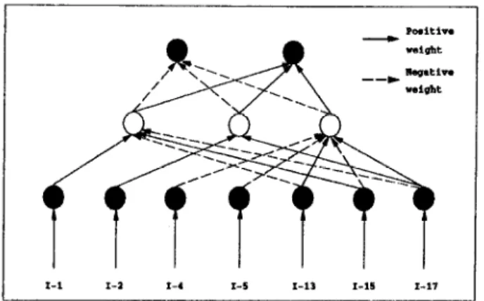
Figure 3 shows the pruned network. Of the 386 links in the original network, only 17 remained in the pruned network. One of the four hidden nodes was removed. A small number of links from the input nodes to the hidden nodes made it possible to extract compact rules with the same accuracy level its the neural network.

3 Extracting

rules from a neural

net-

work

Network pruning results in a relatively simple network. In the example shown in the last section, the pruned network has only 7 input nodes, 3 hidden nodes, and 2 output nodes. The number of links is 17. However, it is still very difficult to articulate the network, i.e., find the explicit relationship between the input tuples and the output tuples. Research work in this area has

Figure 3: Pruned network for Function 2. Its accuracy rate on the 1000 training samples is 96.30 % and it contains only 17 connections.

been reported [25,8]. However, to our best knowledge, there is no method available in the literature that can extract explicit and concise rules as the algorithm we will describe in this section.

3.1 Rule extracting algorithm

A number of reasons contribute to the difficulty of extracting rules from a pruned network. First, even with a pruned network, the links may be still too many to express the relationship between an input tuple and its class label in the form of if.. . then . . . rules. If a node has n input links with binary values, there could be as many as 2n distinct input patterns. The rules could be quite lengthy or complex even with a small R, say 7. Second, the activation values of a hidden node could be anywhere in the range [-l,l] depending on the input tuple. With a large number of testing data, the activation values are virtually continuous. It is rather difficult to derive the explicit relationship between the activation values of the hidden nodes and the output values of a node in the output layer.

Our rule extracting algorithm is outlined in Fig- ure 4.

The algorithm first discretizes the activation values of hidden nodes into a manageable number of discrete values without sacrificing the classification accuracy of the network. A small set of the discrete activation values make it possible to determine both the dependency among the output values and the hidden node values and the dependency among the hidden node activation values and the input values.

From the dependencies, rules can be generated [12]. Here we show the process of extracting rules from the pruned network in Figure 3 obtained for the classification problem Function 2.

(7)

Rde extraction algorithm (RX)

1. Activation value discretization via clustering: (a) Let, E E (0,l). Let D be the number of dis-

crete activation values in the hidden node. Let 51 be the activation value in the hidden node for the first pa.ttern in the tra.ining set. Let W(1) = &,counl(l) = l,sum(l) = Sl and set, D = 1.

(b) For all patterns i = 2,3, . . .Ic in t,he training set:

l Let S be its activation value. l If there exi& an index j such that

and16 - H(?)( 5 E,

then set count(3) := COW@) + 1, sum(D) := sum(D) + s

else D = ll f I., H(D) = 6, counl( D) = 1, sum(D) = 6.

(c) Replace H by the avera.ge of a.11 activation values that have been clustered into this cluster:

H(j) := sum(j)/

coun.t(j), j = 1,2.. .) D. (d) Check the accuracy of the network with the

activa.tion values 6” at the hidden nodes re- placed by Sd, the activation value of the cluster to which the activation value belongs. (e) If the accuracy falls below the required level,

decrease 6 and repeat, Step I.

2. Enumerate the discretized activation values and compute the network output.

Generate perfect rules that have a perfect cover of all the tuples from the hidden node activation values to the output vnlues.

3. For the discretized hidden node activation values a,ppea.red in the rules found in the above step, enumera.te the input values tha.t lead to them, and generate perfect rules.

4. Generate rules that relating the input values and the output values by rule substitution based on the results of the above two steps.

Figure 4: Rule extraction algorit,hm (RX)

Function 2 (Figure 3) had three hidden nodes. The activation values of 1000 tuples were discretized. The value of E was set to 0.6. The results of discretization are shown in the following table.

Node No of clust,ers Cluster activation values

1 3 (-1, 0, 1)

2 2 ( 07 1)

3 3 (-1, 0.24, 1)

The clnssificat~ion accumcy of the network was checked by replacing t,he individual activa.tion value with its diocretized a.ctivation value. The value of 6 = 0.6 was sufficiently small to preserve the accuracy of the neural network and large enough to ha.ve a small number of clusters. For the three hidden nodes, the numbers of discrete activation values (clusters) are 3,2 and 3, or a total of 18 different outcomes art the two output nodes. We tabulate the outputs Crj(l < j 5 2) of the network according to the hidden node activation values (Y,, (1 < m 5 3) a¶ follows.

01 Q2 a3 (71 c2 -1 1 -1 0.92 0.08 -1 1 1 0.00 1.00 -1 1 0.24 0.01 0.99 -1 0 -1. 1.00 0.00 -1 0 1 0.11 0.89 -1 0 0.24 0.93 0.07 I 1 -1 0.00 1.00 1 1 1 0.00 1.00 1 1 0.24 0.00 1.00 1 0 -I 0.89 0.11 1 0 1 0.00 1.00 1 0 0.24 0.00 1.00 0 1 -1 0.18 0.82 0 1 1 0.00 1.00 0 1 0.24 0.00 1.00 0 0 -1 1.00 0.00 0 0 1 0.00 1.00 0 0 0.24 0.18 0.82

Following Algorithm R.X step 2, the predicted outputs of the network are ta.ken to be Cl = 1 a.nd C’s = 0 if the activation values ana’s satisfy one of the following conditions (since the table is small, the rules can be checked manually if interested):

R~l:C1=1,CI,=O e (Y:!=o,a3=-1.

ltl2:c1=1,c2=0 e (Y1=-1,(z2=1,a3=-1. R13:C1=1,C~=0 -S cr1=-1,(~2=O,ng=0.24. Otherwise, Cl = 0 and C2 = I.

(8)

The activation values of a hidden node are determined by the inputs connected to it. In particular, the three activation values of hidden node 1 are determined by 4 inputs, Zi, 213, Zls, and 217. The activation values of hidden node 2 are determined by 2 inputs Z2 and 217, and the activation values of hidden node 3 are determined by &,Zz,Zis,Ziz and 217. Note that only 5 different activation values appear in the above three rules. Following Algorithm RX step 3, we obtain rules that show how a hidden node is activated for the five different activation values at the three hidden nodes:

Hidden node 1: R21 : a1 = -1 e 213= 1 R22 : al= -1 e Zl =213=x15 = 0, 217= 1 Hidden node 2: R23 : 02 = 1 e Zz=l R24 : 02 = 1 -i= 217= 1 Rz5 : 02 = 0 G Zz=Zi7=O Hidden node 3: R2ti : a3 = -1 x= x13=0 R27 : a3 = -1 -t= x5=215= 1 R2a :

a3 = 0.24

e= Z4 = I13 = 1, 217 = 0 Rm: (~3

= 0.24 G

Z5 = 0, 113 = Xl5

= 1

With all the intermediate rules obtained above, we can derive the classification rules as in Algorithm RX step 4. For example, substituting rule

R11

with rules

R25, R26,

and

R27,

we have the following two rules in terms of the original inputs:

Rl:Ci=l,Cz=O + Z2=Z17=0,&3=0

R; : Cl =

l,Cz = 0 + x2 = Zi7 = 0,&j = Z15 = 1 Recall that the input values of 214 to 11s represent coded age groups where 215 = 1 if age is in [60, 80) and 217 = 1 if age is in [20, 40). Therefore rule

Ri

is in fact can never be satisfied by any tuples, hence redundant.

Similarly, replacing rule

Rn

with

RZI, R22,

l&s, Rz4,

R26

and

R27,

we have the following two rules:

R2 : Cl

=l,Cz=O .& 25=213=215=1.

R3

: Cl = 1, Cz = 0 e Zi = Z13 = Z15 = 0,217 = 1.

Substituting

R13

with

R21, Rzz,R25, R28

and

Rzg,

we have another rule:

R4:Ci=l,Cz=O e 22=217=O,Z4=Z13=1.

It is now trivial to obtain the rules in terms of the original attributes. Conditions of the rules after substitution can be rewritten in terms of the original attributes and classification problem as shown in Fig- ure 5.

Given the fact that salary 1 75000 e commission = 0, the above four rules obtained by the pruned network are identical to the classification Function 2.

3.2 Hidden node splitting and creation of a subnetwork

After network pruning and activation value discretization, rules can be extracted by examining the possible combinations in the network outputs as shown in the previous section. However, when there are still too many connections between a hidden node and input nodes, it is not trivial to extract rules, even if we can, the rules may not be easy to understand. To address the problem, a three layer feedforward subnetwork can be employed to simplify rule extra&ion for the hidden node. The number of output nodes of this subnetwork is the number of discrete values of the hidden node, while the input nodes are those connected to the hidden node in the original network. Tuples in the training set are grouped according to their discretized activation values. Given

d

discrete activation values &,Da,..-, Dd, all training tuples with activation values equal to Dj are given a d-dimensional target value of all zeros expect for one 1 in position j. A new hidden layer is introduced for this subnetwork. This subnetwork is trained and pruned in the same ways as is the original network. The rule extracting process is applied for the subnetwork to obtain the rules describing the input and the discretized activation values.

This process is applied recursively to those hidden nodes with too many input links until the number of connection is small enough or the new subnetwork can- not simplify the connections between the inputs and the hidden node at the higher level. For most problems that we have solved, this step is not necessary. One problem where this step is required by the algorithm is for a genetic classification problem with 60 attributes. The details of the experiment can be found in [21].

4 Preliminary

experimental

results

Unlike the pattern classification research in the AI community where a set of classic problems have been studied by a large number of researchers, fewer well documented benchmark problems are available for data mining. In this section, we report the experimental results of applying the approach described in the previous sections to the data mining problem defined in [2]. As mentioned earlier, the database tuples consisted of nine attributes (See Table 1). Ten classification functions of Agrawal et al. [2] were used to generate classification problems with different complexi- ties. The training set consisted of 1000 tuples and the testing data sets had 1000 tuples. Efforts were made

(9)

- Rule 1.

Rule 2.

If (salary < 100000) A (commission = 0) A (age 5 40), then Group A. If (salary 1 25000) A (

R.ule 3. If (salary < 125000) A

commission > 0) A (age >_ 60), lhen Group A.

(

Rule 4.

commission = 0) A (40 5 age < 60), then Group A. If (50000 < salary < 100000) A (age < 40), then Group A.

Default Rule. Group B.

ITigure 5: Rnles generated by NeuroRule for Function 2.

to generate the data sets as described in t,he original functions. Among 10 fmlctions described, we found t#hat function 8 and LO produced highly skewed data that made classifica.tion not mea,ningful. We will only discuss functions other than these two functions. To

assess our approach, we compare the results with that, of C4.5, a decision tree-based classifier [16].

4.1 Classification accuracy

The fnllowing ta.ble reports the classificatiou accuracy using both our system and C4.5 for eight funct,ions. Here, classification accuracy is defined a,9

accrrracy = no tuples correctly classi jied lotal number of tlnples (6)

- F’runed Networks Training 11 Testing 98.1 100.0 96.3 100.0 98.5 100.0 90.6 92.9 90.4 93.1 90.1 90.9 91.9 91.4 90.1 90.9 Tmining 11 Testing 98.3 100.0 98.7 96.0 99.5 99.1 94.0 89.7 96.8 94.4 94.0 91.7 98.1 93.6 94.4 91.8 From the table we can see that the classification accuracy of the neural net,work based approach and C4.5 is comparable. In fa.ct, the network obtained after the training phase has higher accuracy than what listed here, which is mainly determined by the threshold set for the network pruning phase. In our experiments, it is set, bo 90%. That is, a network will be pruned u&i1 further pruning will cause the accuracy to fall below this threshold. For applications where high classification accuracy is desired, the threshold can be set higher so that less nodes and links will be pruned. Of course, this may lead to more complex claqsificatiou rules. Tradeoff between the accuracy and the com- plexit,y of the classification rule set is one of the design issues.

4.2 R.des extracted

Here we present. some of the classification rules cx- tracted from our experiments.

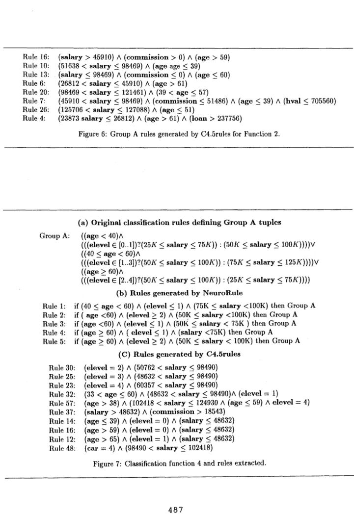
For simple classification functions, the rules cx- tracted are exactly the same <as the classification functions. These include functions 1, 2 and 3. One in- t.eresting example is Function 2. The Mailed process of finding the classification rules is described as an example in Section 2 and 3. The resulting rules are the same as the original functions. As reported by Agrawal it cnl. [2], lD3 generated a. rela.tivcly la.rge number of strings for Function 2 whrn the decision tree is built. We observed similar results when (:Li.Srules was used (a memhcr of ID3). C4.5rules generat.cd 18 rules. Among the 18 rules, 8 rules define the conditions for Group A. Another 10 rules define Group 11. Tuples that do not sa,tisfy the conditions specified a.re classified as default, class, Group B. Figure 6 shows the rules that define tuples to be a member of Group A.

By comparing the rules generated by C4.5rllles (Figure 6) with the rules generated by NeuroR.ule in Figure 4, it is obvious that our approach gcnrrates better rules in the sense that they are more compact., which makes t,he verification and applica.tion of t.hc> rules much ea.sier .

Functions 4 and 5 are anothrr two funct,ious for which ID3 generates a la.rge number of strings. CVDP [2] also g enera,es a relatively t large number of strings than for ot,her functions. The original classification funct,ion 4, the rule sets that, define Group A tuples extracted using NeuroRule and C4.5, respcc- tively are shown in Figure 7.

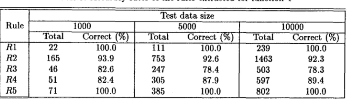
The five rules extracted by NeuroRute are not exactly the same as the original function descriptions (Function 4). To test the rules extracted, the rules were applied to t,hree dat,a sets of different sizes, shown in Table 3. The column Total is the total number of t#uples that, are classified as group A by each rule. ‘1’11~ column Correct is the percentage of correctly classified tuples. E.g., rule RL classifies all tuples correctly. On the other hand, among 165 tuples that, were classified a.s Group A by rule Ra, 6.1% of the~n in fact, should belong to Group R, i.e. they were misclassified.

(10)

Rule 16: R.ule 10: R.ule 13: Rule 6: Rule 20: Rule 7: Rule 26: Rule 4:

(salary > 45910) A ( commission > 0) A (age > 59) (51638 < salary 5 98469) A (age age 5 39)

(salary 5 98469) A ( commission 5 0) A (age < 60) (26812 < salary 5 45910) A (age > 61)

(98469 < salary 5 121461) A (39 < age 5 57)

(45910 < salary 5 98469) A ( commission 5 51486) A (age < 39) A (hval 5 705560) (125706 < salary 5 127088) A (age < 51)

(23873 salary 5 26812) A (age > 61) A (loan > 237756)

Figure 6: Group A rules generat,ed by C4.5rules for Function 2.

(a) Original classification rules defining Group A tuples Group A: ((age < 40)A

(((elevel E [0..1])?(2511 5 salary L: 75Ji)) : (501< 5 salary < 1OOK))))V ((40 5 age < 60)A

(((elevel E [1..3])?(501< < salary 5 lOOI<)) : (751< 5 salary 5 125K))))V ((age L 6O)A

(((elevel E [2..4])?(501- 5 salary 5 lOOIT)) : (251i; 5 salary 5 7510))) (b) Rules generated by NeuroRule

Rule 1: if (40 5 age < 60) A ( .l e eve1 5 1) A (75K 5 salary <lOOK) then Group A Rule 2: if ( age <60) A ( .l e eve1 2 2) A (5Oy 5 salary <lOOK) then Group A Rule 3: if (age <60) A (elevel < I.) A (50K 5 salary < 75K ) then Group A Rule 4: if (age 2 60) A ( 1 e eve1 5 1) A (salary <75K) then Group A

Rule 5: if (age 1 60) A ( e eve1 2 2) A (50K < salary < 100K) then Group A 1 (C) Rules generated by C4.5rules

Rule 30: Rule 25: Rule 23: Rule 32: Rule 57: Rule 37: Rule 14: Rule 16: Rule 12: Rule 48: (elevel = 2) A (50762 < salary 5 98490) (elevel = 3) A (48632 < salary 5 98490) (elevel = 4) A (60357 < salary 5 98490)

(33 < age < 60) A (48632 < salary < 98490)A (elevel = 1)

(age > 38) A (102418 < salary < 124930 A (age 5 59) A elevel = 4) (salary > 48632) A ( commission > 18543)

(age 5 39) A (elevel = 0) A (salary < 48632) (age > 59) A (elevel = 0) A (salary 5 48632) (age > 65) A (elevel = 1) A (salary 5 48632) (car = 4) A (98490 < salary 5 102418)

Figure 7: Classification function 4 and rules extracted.

(11)

Table 3: Accuracy rates of the rules extracted for function 4 Rule Rl R2 R3 R4 R5

Test data size

1000 5000 10000

Total Correct (%) Total Correct (%) Total Correct (%)

22 100.0 111 100.0 239 100.0

165 93.9 753 92.6 1463 92.3

46 82.6 247 78.4 503 78.3

51 82.4 305 87.9 597 89.4

71 100.0 385 100.0 802 100.0

From Table 3 , we can see that two of the rules extracted classify the tuples correctly without errors. They are exactly the same as some rules in the original functions. Because the accuracy of the pruned network is not lOO%, other rules extracted are not the same as the original ones. However, the rule extracting phase preserves the classification accuracy of the pruned network. It is expected that, with higher accuracy of the network, the accuracy of the extracted rules will be also improved.

When the same training data set was used as the input of C4.5rules, twenty rules were generated among which 10 rules define the conditions of Group A (Figure 7). Again, we can see that NeuroRule generates better rules than C4.5rules. Furthermore, rules generated by NeuroRule only reference those attributes appeared in the original classification functions. C4.5rules in fact picked some attributes, e.g. car , that does not appear in the original function. 5

Conclusion

In this paper we reported NeuroRule, a connectionist approach to mining classification rules from given da.tabases. The approach consists of three phases: (1) training a neural network that correc0y classifies tuples in the given training data set to required accuracy; (2) pruning the network while maintaining the classification accuracy; and (3) extracting explicit rules from the pruned network. The proposed approach was applied to a set of classification problems. The results of applying it to a data mining problem defined in [2] was discussed in detail. The results indicate that, US-

ing the proposed approach, high quality rules can be discovered from the given ten data sets. While con- siderable work on using neural networks for classification has been reported, none of them can generate rules with the quality comparable to those generated by NeuroRule.

The work reported here is our first attempt to apply the connectionist approach to data mining. A number of related issues are to be further studied. One of

the issues is to reduce the training time of neural networks. Although we have been improving the speed of network training by developing fast algorithms, the time required for NeuroRule is still longer than the time needed by the symbolic approach, such as C4.5. As the long initial training time of a network may be tolerable, incremental training and rule extracting during the life time of an application database seems important. With incremental training that requires less time, the accuracy of rules extracted can be improved along with the change of database contents.

References

PI

[31 PI I51

PI

[71

R. Agrawal, S. Ghosh, T. Imielinski, B. Iyer, and A. Swami. An interval classifier for database mining approaches. In Proceedings of the 18th VLDB

Conference, 1992.

R. Agrawal, T. Imielinski, and A. Swami. Database mining: A performance perspective. IEEE Tmns. on Knowledge and Data Engineer- ing, 5(6), December 1993.

T. Ash. Dynamic node creation in backpropga- tion networks. Connection Science, 1(4):365-375, 1989.

R. Battiti. First- and second-order methods for learning: between steepest descent and newton’s method. Neuml Computation, 4:141-166, 1992. N. Cercone and M Tsuchiya. Geust editors, special issue on learning and discovery in databases. IEEE Tmns. on Knowledge and Data Engineer- ing, 5(6), December 1993.

J.E. Dennis Jr. and R.B. Schnabel. Numerical methods for unconstmined optimization and non- linear equations. Prentic Hall, Englewood Cliffs, NJ, 1983.

W. Frawley, G. Piatetsky-

Shapiro, and C. Matheus. Knowledge discovery in databases: An overview. AI Magazine, Fall 1992.

(12)

[8] 1,. I%. Neural Networks in Computer Intelligence. McGraw-Hill, 1994.

[9] .J. Han, Y. Cai, and H. Cercone. Knowledge discovery in databases: An attribute oriented approach. In Proceedings of the VLDB conference, pages 547-559, 1992.

[lo] d. Hertz, A. Krogh, and R.G. Palmer. lntroduc- tion to the theory of neural computation. Addison- Wesley Pub. Company, 1991.

[l I] Y. Hirose, K. Yamashita, and S. Hijiya. Back- propagation algorithm which varies the number of hidden units. Neural Networks, 4:61-66, 1991. [12] H. Liu. X2R: A fa.st rule generator In Pm- ceedings of IEEE International Conference on Systems, Man and Cybernetics (SMC’95), Va.n- courver, 1995.

[13] C.J. M th a, eus, P.K. Chan, and G. Piatetsky- Shapiro. Systems for knowledge discovery in da.tabases. IEEE I’mns. on I(tlourledge and Data Engineering, 5(6), December 1993.

[14] G. Piatetsky-Sha.piro. Editor, special isssue on knowledge discovery in databases. International Journal of Intelligent Systems, 7(7), September 1992.

[15] G. Piatetsky-Shapiro. Guest editor introduction: Knowledge discovery in databases - from research to applicat,ions. International Journal of Intelli- gent Systems, 5(l), January 1995.

[16] J.R. Quinlan. C4.5: Programs for Machine Learning. Morgan Kaufmann, 1993.

[I.7 J.R. Quinlan. Comparing connectionist and symbolic learning methods. In S.J. Hanson, G.A. Drastall, and R.L. Rivest, editors, Computational Learning Therory and Natural Learning Systema, volume 1, pages 445-456. A Bradford Book, The MIT Press, 1994.

[18] S. Russell a.nd P. Norvig. Artificial Intelligence: A Modern Approach. Prentic Hall, 1995.

[19] R. Set,iono. A neural network construction algorithm which maximizes the likelihood function. Submitted for publication, 1994.

[20] R. Setiono. A penalty function approach for pruning feedforward neural networks. Subm.itted for publication, 1994.

121

R. Setiono. Extractiug rules from neural network by pruning and hidden unit splitting. Submitted for publication, 1994.

[22] R. Setiono and H. Liu. Improving backpropga- tion learning with feature selection. Applied In- telligence to appear, 1995.

[23] D.F. Sha.nno and K.H. Phua. Algorithm 500: Minimization of unconstrained multivariate func- tious. ACM Tmnsaction on Mathematical Soft- ware, 2(1):87-96, 1976.

[24] J.W. Shavlik, R.J. Mooney, and G.G. Towell. Symbolic and neural learning algorithms: An experimental comparison. Machine Learning, 6(2):111-143, 1991.

[25] G.G. Towell and J.W. Shavlik. Extracting refined rules from knowledge-based neural networks. Ma- chine Learning, 13(1):71-101, 1993.

[26] A. van Ooyen and Nienhuis B. Improving the convergence of the backpropa.gation algorithm. Neu- ml Networks, 5:465-471, 1992.

[27] R.L. Watrous. Learning algorithms for connectionist networks: Applied gradient methods for nonlinear optimization. In Proceedings of IEEE First International Conference on Neural Net- works, pages 619-627. IEEE Press, New York, 1987.

[28] Shalom M. Weiss and Casimir A. Kulikowski. Computer Systems That Learn. Morgan Kauf- mann Publishers, San Mateo, California, 1991.