High Dimensional Yield Curves: Models and Forecasting

High Dimensional Yield Curves: Models and Forecasting

and Roland Meeks

Nuffield College, University of Oxford, Oxford, OX1 1NF, U.K. [email protected]

[email protected] October 2, 2006

Abstract

Functional Signal plus Noise (FSN) models are proposed for analysing the dynamics of a large cross-section of yields or asset prices in which contemporaneous observations are functionally related. The FSN models are used to forecast high dimensional yield curves for US Treasury bonds at the one month ahead horizon. The models achieve large reductions in mean square forecast errors relative to a random walk for yields and readily dominate both the Diebold and Li (2006) and random walk forecasts across all maturities studied. We show that the Expectations Theory (ET) of the term structure completely determines the conditional mean of any zero-coupon yield curve. This enables a novel evaluation of the ET in which its 1-step ahead forecasts are compared with those of rival methods such as the FSN models, with the results strongly supporting the growing body of empirical evidence against the ET. Yield spreads do provide important information for forecasting the yield curve, especially in the case of shorter maturities, but not in the manner prescribed by the Expectations Theory.

Keywords: Yield curve, term structure, expectations theory, FSN models, functional time series, forecasting, state space form, cubic spline.

JEL classification: C33, C51, C53, E47, G12.

1

Introduction

In this paper we develop a novel econometric framework for modelling and forecasting high dimensional yield curves consisting of the yields on a large number of discount bonds with different maturities. Forecasting one month ahead, we are able to improve upon the forecasting performance of all other existing methods, including a new method introduced here in which the forecasts implement the conditional mean implied by the expectations theory of the term structure. Two obvious lacunae exist in the term structure literature: the vast majority of empirical dynamic studies concentrate on a small subset of maturities rather than entire term structures; and there is a relative paucity of work concerned primarily with forecasting the yield ∗_{Corresponding author: tel: +44 1865 278969, fax: +44 1865 278621. Comments are welcome and should}

be directed to the above e-mail address. Functional Signal plus Noise (FSN) models were first introduced in the earlier working paper, Bowsher (2004).

curve. The first stems from the econometric difficulties involved in modelling the dynamics of a high dimensional cross-section of interest rates that are functionally related to one another. The second exists despite the considerable importance of forecasting the term structure for bond portfolio management, derivatives pricing and monetary policy. The methods introduced here address both areas and can also readily be applied to time series of other economically important functions such as the supply and demand curves of the limit order book of a financial exchange (see Bowsher 2004).

The main contributions of the paper may be summarised as follows. First,Functional Signal plus Noise (FSN) time series models are introduced for analysing the dynamics of a large cross-section of yields or asset prices in which contemporaneous observations are functionally related. The FSN models specify the evolution over time of stochastic functions, a problem that has received relatively little attention in the econometrics and statistics literature, and the models may conveniently be written in linear state space form. Second, we show that the Expectations Theory (ET) of the term structure completely determines the conditional mean of any zero-coupon yield curve, given an information set that includes the currently observed, complete yield curve of adequate dimension. We are thus able to derive and implement the minimal mean square error point forecasts implied by the theory. Third, FSN models are used to forecast high-dimensional yield curves for US Treasury bonds at the 1 month ahead horizon and their performance compared in an out-of-sample experiment to the ET forecasts and the Diebold and Li (2006) dynamic Nelson-Siegel model. The preferred FSN models achieve large reductions in mean square forecast error (MSFE) relative to a random walk for the yield curve, especially at the shorter maturity end, and readily dominate the ET, Diebold and Li (2006), and random walk forecasts in terms of MSFE across all maturities studied. A novel and particularly direct evaluation of the ET is thus also provided in which its 1-step ahead forecasts are compared with those of rival models. Our results, obtained using two different datasets, strongly support the growing body of empirical evidence against the ET.

In the Functional Signal plus Noise models developed here, the information about the func-tional, cross-sectional relationship between contemporaneously observed yields is captured by modelling the observed curves as the sum of a smooth ‘signal function’ or latent yield curve, S(τ), and noise. The signal function used is a cubic spline uniquely determined by the yields

that correspond to the knots of the spline, theknot-yields. The state equation of the FSN model then determines the stochastic evolution of the spline function by specifying that the knot-yields follow a vector autoregression which may be written as an equilibrium correction model (ECM) in which the spreads between the knot-yields appear as regressors. We find that yield spreads provide important information for forecasting the yield curve, especially in the case of shorter maturities, but not in the manner prescribed by the ET.

The work presented is also a contribution to applied functional time series analysis. Each yield curve may be regarded as a finite dimensional vector, albeit of very high dimension. How-ever, the standard approaches of multivariate time series or panel data econometrics are of little help in this setting, owing to the high dimensionality of the curves and the close, functional relationship between the yields. Indeed, the analysis of time series of stochastic functions is in a state of relative infancy.1 Previous work in the statistics literature includes the use of Functional AutoRegressive (FAR) models for forecasting entire smooth, continuous functions by Besse and Cardot (1996) and Besse, Cardot, and Stephenson (2000). The FSN models may be interpreted as a special type of dynamic factor model (see Stock and Watson 2006, pp. 524) in which the knot-yields are the factors and the factor loadings are determined by the requirement that the latent yield curve (i.e. the vector of ‘common components’) be a natural cubic spline function, rather than the factor loadings being parameters for estimation. The semiparametric FSN approach thus allows quasi-maximum likelihood estimation using the state space form and the Kalman filter even when the cross-sectional dimension of the data is very large.

Two previous studies examine out-of-sample forecasting of high dimensional yield curve functions. Diebold and Li (2006) introduce a dynamic version of the Nelson and Siegel (1987) yield curve in which the three parameters or factors describing the curve each follow an AR(1) process. They report only comparable forecasting performance to that of a random walk for the yield curve (denoted RWY C_{) in terms of MSFEs at the 1 month ahead forecast horizon, but}

substantial improvement in MSFEs over the RWY C and other benchmark forecasting models at a horizon of 12 months. Kargin and Onatski (2004) forecast approximate forward rate curves (derived from Eurodollar futures rates) 1 year ahead using a functional autoregression and their new predictive factor decomposition. They uniformly outperform the MSFEs of the Diebold and

1

Functional Data Analysis by Ramsay and Silverman (1997) is a landmark in this area but does not consider the time series case in which the functions are dependent.

Li (2006) and RWY C procedures across all maturities, but report small reductions in MSFEs relative to the forecast based on the average yield curve observed to date.

The two studies reflect a common theme in the term structure literature, namely the difficulty of outperforming na¨ıve forecasting devices, particularly the RWY C or ‘no change’ forecast. Duffee (2002) documents that forecasts made using the standard class of (‘completely’) affine term structure models typically perform worse than the RWY C _{at horizons of 3, 6 and 12 months}

ahead. His ‘essentially affine’ models produce forecasts somewhat better than the RWY C for the three maturities reported and at all 3 horizons. Ang and Piazzesi (2003) present a VAR model in the affine class for yields of 5 different maturities which imposes no-arbitrage restrictions and performs slightly better than the RWY C at the 1 month ahead forecast horizon for 4 of the 5 maturities used. Incorporating macoreconomic factors in the model further improves the forecast performance for those 4 maturities. Finally, Swanson and White (1995) show that the premium of the forward rate over the 1 month short rate, and lags thereof, can be used to improve the 1-step ahead MSFE of the 1 month rate relative to a random walk with drift.

For the first time in the literature, we present forecasting models whose 1 month ahead forecasts strongly outperform a random walk for the yield curve. Furthermore, the models are for high dimensional yield curves rather than for a small subset of maturities. The structure of the paper is as follows. Section 2 develops two new methods for modelling and forecasting high dimensional yield curves – FSN models and forecasts based on the Expectations Theory of the term structure. Theorem 1 contains our result on the conditional expectation of yield curves under the ET. A procedure for evaluating the ET based on Theorem 1 is also proposed and previous empirical work in this area reviewed. Section 3 applies both methods to the task of forecasting high dimensional US Treasury zero-coupon yield curves, whilst Section 4 focuses on forecasting a complete set of US Treasury bill yields. Section 5 then concludes. The Appendix provides the necessary mathematical details on cubic spline functions. These are denoted here, as a function of maturity τ, byS(τ).

2

Models for High Dimensional Yield Curves

A zero-coupon or discount bond with face value $1 and maturity τ is a security that makes a single payment of $1 τ periods from today. Its yield to maturity, yt(τ), is defined as the per

period, continuously compounded return obtained by holding the bond from time tto t+τ, so that

yt(τ) =−τ−1pt(τ), (1)

where pt(τ) is the log price of the bond at t. The (zero-coupon) yield curve consists of the

yields on discount bonds of different maturities and is denoted generically here by the vector

yt(τ) := (y_t(τ₁), y_t(τ₂), ..., y_t(τ_N))′.The purpose of the current paper is to develop forecasting

methods for the empirically relevant case where the cross-sectional dimensionN of the observed yield curve is large. In Section 3 the task will be to forecast one month ahead a 36×1 yield curve with τ = (1.5,2,3, ...,11,12,15,18, ...,81,84) and where maturities are measured in months. A

3-dimensional plot of the dataset used there may usefully be previewed at this stage by examining the first panel of Figure 2. The plot strongly suggests the suitability of treating each observed yield curve as a smooth function perturbed by noise. Taking the contemporaneous pairwise correlations of yields for adjacent maturities using the dataset shown there gives correlations that all lie between 0.9964 and 0.9997.

In this section we present two new approaches to such a forecasting problem. First we describe the flexible, semiparametric family of Functional Signal plus Noise models. Second, we ask what the Expectations Theory of the term structure implies about forecasting yields when a history of complete yield curves is available upon which to base the forecasts. An n -dimensional yield curve is said to be complete here when yields are observed for all maturities

τ ∈ {1,2, ..., n}. In the dataset of Section 3, complete yield curves are available with n = 85. It turns out that the ET completely determines the conditional mean of any yield curve yt(τ),

no matter how large its dimension, given an information set that includes the current, complete (τN+ 1)-dimensional yield curve. In a comparison of the forecast performance of the FSN model

and ET forecasts in Section 3, we find that the FSN models prove very effective in forecasting high dimensional yield curves, whilst the conditional mean implied by the ET does not give the MSFE-minimising point forecasts of the yields.

2.1 Functional Signal plus Noise Models

In the semiparametric Functional Signal plus Noise models proposed here, the information about the functional, cross-sectional relationship between contemporaneously observed yields is

cap-tured by modelling the observed curves as the sum of a smooth latent ‘signal function’, S(τ),

and noise. The exposition below is given in terms of yield curves. However, the FSN models can also readily be applied to time series of other economically important functions such as the supply and demand curves of an electronic limit order book (see Bowsher 2004).

The signal function used is a cubic spline uniquely determined by the yields that correspond to the knots of the spline, the knot-yields. The state equation of the FSN model then determines the stochastic evolution of the spline function by specifying that the knot-yields follow a vector autoregression which may be written as an equilibrium correction model (ECM) in which the spreads between the knot-yields appear as regressors. It is shown how to write the FSN-ECM model in linear state space form, thus allowing the use of the Kalman filter to compute both the Gaussian quasi-likelihood function and one-step ahead point predictions.2 _{Harvey and Koopman} (1993) were the first to describe a linear state space model with a state equation determining the stochastic evolution of a cubic spline function. There, as in Koopman and Ooms (2001), the stochastic spline is used to model the latent, time-varying periodic pattern of a scalar time series. This contrasts the present work in which the stochastic splines are used as a tool in functional time series analysis and assume the role of smooth approximations to the observed functional data.

2.1.1 FSN-ECM models

The FSN-ECM model consists of a dynamically evolving, natural cubic spline signal function denoted bySγt(τ),plus a noise process. A cubic spline is essentially a piecewise cubic function with pieces that join together to form a smooth function overall.3 _{The spline signal function} or latent yield curve,Sγt(τ) := (Sγt(τ1), ..., Sγt(τN))

′

,hasm knots positioned at the maturities

k= (1, k2, ..., km), which are deterministic and fixed over time. The notation Sγt(τ) is used to imply that the spline interpolates to the latent yieldsγ_t= (γ_1t, ..., γ_mt)′

– i.e. Sγt(kj) =γjt for

j = 1, ..., m. We refer to the vector γ_t as the knot yields of the spline. An illustrative spline signal function is shown in Figure 1. Another terminology is to refer to Sγt(τ) as a natural cubic spline on (k;γ_t), since the spline passes through the points (kj, γjt)mj=1, which together

2

The termKalman filter should always be taken here to refer to the recursions as they are conveniently stated in Koopman, Shephard, and Doornik (1999, Section 4.3, pp. 122-123). For a textbook exposition of the Kalman filtering procedure, see Harvey (1989, Ch. 3).

3

0 10 20 30 40 50 60 70 80 1 2 3 4 5 6 7 8 9 S_γ t(τ ) γ_5t γ_4t γ_3t γ_2t γ_6t γ_1t maturity

Figure 1: An illustrative spline signal function or latent yield curve, Sγt(τ). The yields at the

knots,γjt, are labelled and plotted using filled circles; the knots are given byk= (1,2,4,18,24,84).

determine the remainder of the spline function uniquely. A formal definition of the FSN-ECM model now follows.

Definition 1 FSN-ECM Model. The model for the time series ofN-dimensional observed yield curves, {yt(τ)},is given by

yt(τ) = S_γ

t(τ) +ǫt = W(k,τ)γ

t+ǫt, (2)

∆γ_t+1 = α(β′γ_t−µ_s) + Ψ∆γ_t+νt, (3) for t= 1, ..., T. Here Sγt(τ)is a natural cubic spline on (k;γt),the N×mdeterministic matrix

W(k,τ) is given by Theorem 2 of the Appendix, the m×(m−1) matrix α has full rank, and

the matrix β is defined uniquely by β′γ_t= (γ_j+1,t−γ_jt)m_j=1−1. The initial state (γ′

1, γ

′

0)

′

has finite first and second moments given byµ∗

andΩ∗

respectively.The series{ut:= (ǫ′t, ν ′ t)

′

}has a finite second moment for allt and satisfies, for allt, E_{[ut] = 0,}E_[ǫtǫ′_{t] = Ωǫ,}E_[νtν′_{t] = Ων,}E_[ǫtν′_{t] = 0,} E_[utu′

s] = 0∀s6=t, and E[ut(γ′1, γ

′

The Gaussian FSN-ECM Model is the FSN-ECM model with the additional condition imposed that both ut and(γ′1, γ

′

0)

′

have multivariate Normal distributions.

The state equation (3) is motivated by the cointegration-based yield curve literature discussed in Section 2.2.1 and is consistent with the case where the knot yieldsγ_tare I(1) and the (m−1) spreads between them are cointegrating relations.4 In that case, E_{[∆γt+1] = 0 which excludes}

deterministic trends, and µ_s = E_[β′_γ

t], the stationary mean of the spreads. Furthermore the N-dimensional latent yield curve, Sγt(τ), is in that case I(1) and itself has (N −1) linearly independent, stationary yield spreads which are cointegrating relations.

Under the conditions of Definition 1, the FSN-ECM model can be written in linear state space form, as defined by Harvey (1989, pp. 100-104). It is important to note that the deterministic matrixW(k,τ) depends only on the vector of maturitiesτ and the knot positionskthus allowing

the spline signal function Sγt(τ) to be written as the linear function, W(k,τ)γ

t, of the knot

yields. The state vector attcan be taken to be (γ′ t, γ

′ t−₁)

′

or, in an isomorphic representation, to be (γ_1t,(β′ γ_t)′ , γ_1,t−₁,(β ′ γ_t−₁) ′ )′

– see also equation (10). We use the latter in our computational work. The choice of a cubic spline as the signal function in FSN models has two advantageous features. First, the stochastic evolution over time of the signal function is determined completely by the time series properties of the m-dimensional vector γ_t, where m is relatively small (e.g.

m = 5), thus allowing the construction of a parsimonious model when the dimension of the yield curve is very much larger. Second, since the model has the linear state space form, the Kalman filter may be used to perform both quasi-maximum likelihood estimation (QMLE) and 1-step ahead, linear point prediction. These two features, together with the flexibility of cubic splines as approximating functions, make the cubic spline framework adopted here a particularly attractive one.

In Sections 3 and 4, the parameters of the various FSN-ECM models are estimated by max-imising the likelihood of the corresponding Gaussian FSN-ECM model, which may be computed using the Kalman filter and widely available software for state space time series models. This procedure gives the QMLEs for the parameters. The FSN-ECM forecasts for the models used in Sections 3 and 4 are the 1-step ahead point predictions given by the Kalman filter, [ˆyt(τ)|

4

However, we prefer a broader definition of the FSN-ECM model and thus do not impose additional conditions on the roots of the characteristic polynomial of the VAR in (3) and on det[α′

yt−₁(τ), ..., y₁(τ);θ]_KF, with the parameter vector of the model set equal to some estimated

value, θ. Note that [ˆyt(τ)| y_t−₁(τ), ..., y₁(τ);θ]_KF is a linear function of the past observations

(yt−₁(τ), ..., y₁(τ)) and has minimum MSFE amongst the class of such linear predictors whenθ

is equal to the true parameter vector.5 2.2 Expectations Theory Forecasts

Complete n-dimensional yield curves are denoted here by yt(1 : n) := (yt(1), yt(2), ..., yt(n))′.

The vector of spreads between the yields and the short rate is written as snt := (st(2,1), ..., st(n,1))′,wherest(τj, τi) is defined as the spreadyt(τj)−yt(τi). The Expectations Theory states

that a longer-termτ-period yield differs only by a time-invariant constant from the conditionally expected per period log return obtained by successively rolling over 1-period discount bonds for

τ periods.6 _{A formal definition is as follows.}

Definition 2 The Expectations Theory (ET) is the statement that

yt(τ) = ( τ−₁ τ−₁ X i=0 E_[yt+i(1)|Ft] ) +ρ(τ), τ = 1,2, ..., (4)

where the constantsρ(τ)∈R_{are known as term premia,ρ(1) = 0,and{Ft}denotes the filtration} of publicly available information which includes the natural filtration of the yield curve.

Note that in Definition 2 the physical units of time used to measure bond maturity and the time interval between observations are necessarily the same.

Theorem 1 below states that the ET fully determines the conditional expectation of the (n−1)-dimensional yield curve, yt+1(1 : n−1), given any information set that includes the current n-dimensional yield curve, yt(1 : n). Furthermore, that conditional expectation is an

affine function of the current spread vector, snt. The key result is that

E_{[∆yt+1(τ)|Ft] =} τ + 1

τ {st(τ+ 1,1)−ρ(τ+ 1)} − {st(τ ,1)−ρ(τ)}, τ = 1,2, ... (5)

which in matrix form yields the following theorem.

5

Recall that when θ is equal to the truth, [ˆyt(τ)| yt₋1(τ), ..., y1(τ);θ]KF is only guaranteed to equal

Eθ[yt(τ)|yt₋1(τ), ..., y1(τ)] for the Gaussian FSN-ECM model.

6

Campbell, Lo, and MacKinlay (1997, Ch.10) provide a useful summary of different forms of the ET. We follow the majority of the empirical literature by examining the logarithmic form, rather than working with bond prices in dollars and the associated gross yields to maturity.

Theorem 1 (Conditional Expectation of Yield Curve) Let n≥2 and suppose that the Expectations Theory (Definition 2) is satisfied. Then,

yt+1(1 :n−1) =yt(1 :n−1) + ¯αnET−₁(snt−ρn) +νt+1, (6)

where E_{[νt+1|Ft] = 0andρn= (ρ(2), ...,(ρ(n))}′_{. The(n−1)×(n−1)matrix α¯}ET_{n−1 is, forn >2,} given by ¯ αET_n−₁ =        2 0 0 0 . . . 0 0 −1 3/2 0 0 . . . 0 0 0 −1 4/3 0 . . . 0 0 .. . ... ... ... . .. ... ... 0 0 0 0 . . . −1 _n−n₁        , (7)

and α¯ET₁ = 2. It follows from the definition of excess returns on a τ period bond, denoted here byrxt+1(τ), that under the Expectations Theory

E_{[rxt+1(τ)|Ft] =τ ρ(τ)−(τ −1)ρ(τ−1), τ = 2,3, ... (8)}

We prove Theorem 1 elsewhere (see the proof of Theorem 1 of Bowsher and Meeks 2006). The important point to note here is that when one works with a complete term structure of maturities, τ = (1,2, ..., n), the matrix ¯αET

n−₁ and hence the conditional mean of the (n−

1)-dimesional yield curve are both entirely determined by the ET. This has not previously been recognised. Put another way, under the null of the ET alone (i.e. Definition 2), the MSFE-minimising, 1-step ahead forecasts are a known linear function of the difference between the spread and term premia vectors. Note from equation (8) that conditionally expected excess returns from holding aτ period bond for 1 period (that is, in excess of the 1 period yield, yt(1),

and realised at timet+ 1), are deterministic and constant over time under the ET. 2.2.1 Evaluating the ET

Theorem 1 gives an alternative, theory-based approach to forecasting high dimensional yield curves. Note that these yield curves need not be complete. Since E_{[∆yt+1(τ)|Ft] involves the}

spread st(τ + 1,1), the method is feasible provided that the data used to form the forecasts

contains the yields for the required maturities (see equation 5). However, this will not usually create any difficulty. In Sections 3.4 and 4 below, the FSN-ECM model forecasts are compared to these ET forecasts, with the results strongly favouring the former. This not only subjects

the proposed FSN-ECM models to comparison with a broader set of models, but also provides a new method of evaluating the ET.

Under the null of the ET the forecasts implied by (6) have smaller MSFE for each maturity

τ than any other forecasting method since they are based on the conditional mean. Models that outperform the forecasting equation (6) in terms of MSFE thus constitute evidence against the ET. The proposed evaluation method in which the forecasts implied by (6) are compared with those of rival models has several advantages. First, the method is applicable to any dimension of yield curve,N, no matter how large. Second, if the ET is taken to hold no matter what the physical units of timetare in Definition 2, then forecasting equation (6) holds under the null of the ET for any time series frequency (e.g. weekly, monthly or yearly time series). Third, unlike tests of the stationarity of yield spreads which assume that the yield curve is I(1) and hence that the spreads are cointegrating relations under the null of the ET, the method is free of auxiliary ‘nuisance’ assumptions concerning the order of integration of the yield curve.

In contrast to our approach here, the cointegration-based literature seeks to evaluate the ET by analysing the monthly time series of a low dimensionalN-vector of zero-coupon yields, where

N is typically less than 10. Attention usually focuses on inference concerning the cointegration rank and cointegrating relations, with different studies reaching varying conclusions that are sensitive to a largely unknown degree on the subset of maturities chosen. Hall, Anderson, and Granger (1992) find that three linearly independent spreads are cointegrating relations when T-bills with maturities of 1, 2, 3, and 4 months are modelled. Pagan, Hall, and Martin (1996) work with a 5-dimensional yield curve and report rejection of the standard hypothesis test that 4 linearly independent spreads are cointegrating relations. They note however that the point estimates are quite close to the situation where such cointegrating relations hold. These authors also highlight the major impact on the critical values of the test of a levels effect of the short rate in the disturbance of the VAR, which may result in the test rejecting erroneously. Shea (1992) reaches a variety of conclusions depending on which maturities are modelled, finding both cases with 2 common trends and a single common trend. He reports that the cointegrating relations can often be written as linear combinations of the yield spreads.

It is possible to construct DGPs inconsistent with the ET (for example using FSN-ECM processes with Ωǫ = 0) in which the N-dimensional yield curve is I(1) and there are (N −

1) linearly independent spreads that are stationary cointegrating relations, but in which the conditional expectations of the yields do not satisfy Theorem 1. The evaluation method proposed here thus utilises the implications of the ET more fully than cointegration-based approaches which test only a weak implication of the theory, namely that (N −1) linearly independent spreads are cointegrating relations when the yield curve is I(1).

The important regression studies of Fama and Bliss (1987), Campbell and Shiller (1991) and Cochrane and Piazzesi (2005) all find evidence that, contrary to the ET, conditional expected excess returns E_{[rxt+1(τ)|Ft] are stochastic and time varying (cf equation 8). Campbell and}

Shiller (1991) can be interpreted as finding a strong positive effect on E_{[rxt+1(τ)|Ft] of the}

spreadst(τ ,1) forτ ranging from a few months to 10 years, where the time series frequency is

monthly. Fama and Bliss (1987) and Cochrane and Piazzesi (2005) work instead with yearly time series. The important finding is that conditional expected excess returns depend on (one period) forward rates at t, which may be expressed as a linear combination of spreads plus the one period interest rate. Indeed, Cochrane and Piazzesi (2005) find that asingle, ‘tent-shaped’ linear combination of forward rates predicts excess returns on 2 to 5 year maturity bonds realised in 1 year’s time with an R2 _{of up to 0.44. In order to see the connection of these regression} studies with our approach, note that the definition of excess returns implies the identity

E_{[∆yt+1(τ)|Ft] =} τ+ 1

τ st(τ + 1,1)−st(τ ,1)−

1

τE[rxt+1(τ + 1)|Ft], τ = 1,2, ... (9)

Thus, if for example spreads or lagged changes in yields enterE_{[rxt+1(τ+ 1)|Ft], the conditional}

expected change in the yieldE_{[∆yt+1(τ)|Ft] then deviates from the one implied by the ET in (5).}

Indeed, the above regression studies lead us to expect that spreads will be useful in forecasting the yield curve but not in the way prescribed by the ET.

We show later in Sections 3.4 and 4 that the 1-month ahead, out-of-sample forecasts of certain FSN-ECM models have much smaller MSFEs than the ET forecasts based on equation (6), for all maturities forecast in the two datasets examined there (36 different maturities ranging from 1 month to 7 years). The ET forecast errors are also positively autocorrelated at a lag of 1 month, with an average sample autocorrelation of approximately 0.3. We conclude that the conditional mean of Theorem 1 implied by the ET is far from being the optimal MSFE predictor and that the ET is very wide of the mark. Our findings can be interpreted as evidence that conditional

expected excess returns for the one month ahead horizon, E_{[rxt+1(τ)|Ft], are stochastic and}

time varying for maturities τ ranging widely from 1 month to 7 years. The findings are thus complementary to the results reported for the one year ahead horizon in Cochrane and Piazzesi (2005).

3

Forecasting High Dimensional Yield Curves

This section presents the results of an out-of-sample forecasting exercise in which the new FSN-ECM models and ET forecasts are used to forecast high dimensional yield curves and their performance compared to that of the main competing models. The task set is a difficult one, namely to forecast one month ahead a 36×1 dimensional zero-coupon yield curve. The data are first described in detail before moving on to discussion of the specification and selection of the FSN-ECM models used, and the forecasting results obtained.

3.1 Data

We use the same dataset of Unsmoothed Fama Bliss (UFB) forward rates as Diebold and Li (2006), running from November 1984 to December 2000 inclusive. The dataset is available from and has been constructed by Robert Bliss using data from the CRSP government bond files.7 Zero-coupon UFB yields are then obtained by averaging the appropriate UFB forward rates. As is discussed below, the set of maturities for which yields are observed is not the same for every t. Although our FSN-ECM models can readily accommodate this feature using a time-varying but deterministic matrix W(k,τ_t) in the observation equation (3), we work here with

the fixed vector of maturities τ = (1.5,2,3, ...,11,12,15,18, ...,81,84), where maturities are in

months and 1 month is taken to equal 30.4375 days. This approach enables the disaggregation by maturity of forecast performance over time and facilitates comparison with earlier work. Where a yield yt(τi) is not directly observed, a linear interpolation between the two nearest maturity

observations is performed, as in Diebold and Li (2006). Note that we include a greater number of maturities between 1.5 months and 7 years than these authors (36 maturities compared to 14).

A 3-dimensional plot of the final dataset is shown in Figure 2, together with a plot in

7

For further details see Bliss (1997) and the notes accompanying the “Bliss Term Structure Generating Pro-grams.” The latter may be obtained together with our dataset, ufb2full.dat, by request to Robert Bliss.

the lower panel of the maturities directly observed at each date. The latter highlights the clear time-variation in the set of directly observed maturities. The minimum and maximum maturities of 1.5 and 84 months respectively were chosen in order mostly to avoid interpolations using observations separated by a relatively large maturity span. Note in particular that it is difficult to construct a reliable 1 month yield using this dataset since there is frequently no observed maturity less than or equal to 30.4375 days.8 _{Diebold and Li (2006, Table 1) provides} descriptive statistics for a subset of our maturities.

Amongst US government bonds, only Treasury Bills are pure discount bonds whilst others are coupon bearing. Thus the zero-coupon yield curve must first be constructed from the observed bond prices. Bliss (1997) discusses and compares the leading term structure estimation methods and finds that the Unsmoothed Fama Bliss (UFB) method used here performs best overall. The UFB method (see Fama and Bliss 1987, p.690) essentially constructs a piecewise constant forward rate curve, constant over the intervals between the maturities of the included bonds, that exactly prices each bond (under the assumption that coupon bonds are priced as bundles of synthetic discount bonds). All existing studies of yield curve dynamics employ such a cross-sectional estimation of the yield curve prior to and separate from modelling its dynamics.

This is somewhat unsatisfactory from the econometric viewpoint of wishing to model and forecast observable data within a single inferential framework. The FSN framework is ideally suited to this task since it consists of a latent yield curve and data observed with measurement error. One possibility would be to retain the ECM state equation (3) for the latent knot-yields, transform these using the relation in (1) to obtain latent knot-prices, and then form a latent discount function as the natural cubic spline interpolating to those knot-prices. The observation equation is then non-linear, and expresses the observed prices of coupon bonds as a function of the future coupon payments for each included bond, the latent discount function and the measurement error, ǫt. Fitting such a non-linear FSN-ECM model results in estimation of the

discount function using a cubic spline, as in the widely used McCulloch (1971) procedure, but does so by making coherent use of both the time series and cross-sectional information in the data. This extension of our approach would allow forecasting of future coupon bond prices and

8

In the absence of such an observation, there is no valid point to use as the lower maturity point in a linear interpolation. An alternative, not adopted here, would be to derive a 1 month yield by assuming yields are constant for all maturities up to and including the first observed maturity.

Jan−85 Jan−86 Jan−87 Jan−88 Jan−89 Jan−90 Jan−91 Jan−92 Jan−93 Jan−94 Jan−95 Jan−96 Jan−97 Jan−98 Jan−99 Jan−00 Jan−01 20 40 60 80 100 120 140 160 180 Maturity (months)

Jan−85 Jan−86 Jan−87 Jan−88 Jan−89 Jan−90 Jan−91 Jan−92Jan−93_{Jan−94 Jan−95 Jan−96 Jan−97 Jan−98 Jan−99 Jan−00 Jan−01} 20 40 60 80 2 4 6 8 10 12 Maturity (months) Yield (%)

Figure 2: Zero-coupon, Unsmoothed Fama Bliss yields on US Treasury bonds. The upper panel shows a 3-dimensional plot of the dataset used in Section 3; yields are measured in percentage points per annum. The lower panel plots as circles the maturities observed at each date.

is left to future research.

3.2 FSN-ECM forecasting models

The model nomenclature FSN(m)-ECM(p) is used to denote a model in which the spline,Sγt(τ), has knots positioned atmdifferent maturities (i.e. the knot vector khas dimensionm) and the maximum lag entering the ECM state equation (3) is the pth lag of γ_t+1. We consider models here with m ∈ {5,6} and p ∈ {1,2}. The following non-singular transformation of the state equation is useful in what follows. The transformed vector, ϕ_t:=Qγ_t, consisting of the (latent) short rate and inter-knot (latent) yield spreads is given by

ϕ_t:= γ_1t, γ_2t−γ_1t, ..., γ_mt−γ_m−_1,t ′ = 1 01×_(m−₁₎ β′ γ_t=Qγ_t, (10)

whereβ′ is defined as in (3). The state equation may then be written equivalently as the VAR ∆ϕ_t+1=Qα(β′Q−1ϕ_t−µ_s) +QΨQ−1∆ϕ_t+η_t, (11) whereη_t=Qνt, and we define Ωη =Var[ηt] =QΩνQ′.

For all of the FSN(m)-ECM(p) forecasting models used in Sections 3 and 4, the covariance matrix Ωη is diagonal and Ωǫ =σ2ǫIN has the one free parameter, σ2ǫ. In all cases the Kalman

filter is initialised using (γ′

1, γ ′ 0) ′ ∼ (µ∗ ,Ω∗ ), where Ω∗ = 0 and µ∗

is set equal to the yields, (y0(k)′, y−₁(k)′)′, that correspond to the knot maturities and areobserved in the data for the two

periods prior to our estimation period (i.e. 1984:11 and 1984:12).9 _{FSN(m)-ECM(1) models} are obtained by setting Ψ = 0, whilst we impose that QΨQ−₁

is diagonal in all FSN(m )-ECM(2) models. The latter restriction means that only own lagged changes of the short rate and spreads enter each equation in (11). The matrix α in (3) determines the loadings on the spread regressors,β′γ_t. The FSN(5)-ECM(p) models considered always employ an unrestricted

α, whilst the FSN(6)-ECM(p) models use a restricted α in which the first 5 rows form an upper triangular matrix and the last row consists entirely of zeros. We dub this form, which draws on the empirical findings of Hall, Anderson, and Granger (1992), ‘triangular α’ and adopt the nomenclature T-FSN(m)-ECM(p) for models with the restriction imposed. In such triangular

9

The initialisation procedure used legitimately conditions on pre-sample information and avoids augmenting the parameter vector of the model with the initial state vector. Diffuse initialisation was found not to perform well in forecasting in this context. The motivation is the use of the approximation that the observed knot-yields follow a random walk for the 2 periods in question. Note that in Section 3.4 it is necessary to useγ1t=yt₋1(1.5)

models the change in a given knot-yield, ∆γ_j,t+1, depends only on time t spreads involving knot-yields of the same and longer maturities, i.e. on (γ_j+1,t−γ_j,t, ..., γ_m,t−γ_m−_1,t)

′

). Thus, when Ψ = 0, ∆γ_m,t+1 follows a random walk.

3.3 Model selection procedure

The data from 1985:1 to 1993:12 inclusive was used as ‘training’ data for the purpose of an in-sample model selection stage in which the number of knots (m) and their positions (k) were determined. One-step ahead forecasts of the data for each month from 1994:1 to 2000:12 inclusive were then made using a small subset of models carried forward from the in-sample stage, and the forecasts compared across those models. It was felt that there was insufficient data to hold back some time periods for additional evaluation of a single forecasting model or procedure selected after the second stage.

The in-sample stage for knot selection is based on assessing the cross-sectional fit for a large number of different knot vectors, k. Specifically, we fit using OLS a natural cubic spline with knot vectorkto each observed yield curve,yt(τ), and then compute the mean across time of the

residual sum of squares (RSS) from each of the cross-sectional regressions. Form= 5 andm= 6,

the top twenty knot vectors in terms of minimisation of the mean RSS amongst all possiblekwith end knots at 1 and 84 months and internal knots lying in the set (2,3, ...,11,12,15,18, ...,78,81). This is the same set of maturities used in the dataset described above, but excluding the shortest and longest maturities.10 _{Other values of m were not considered. The procedure has the} advantage that it is computationally feasible to search over a very large model space in the manner described (46,376 knot vectors for m= 6, and 5984 for m= 5). The criterion is cross-sectional fit rather than dynamic forecasting, but the ability to mimic the shape of observed yield curves is a preliminary desideratum for the FSN-ECM model to perform well in forecasting. Three knot vectors for m = 6 and one for m = 5 were then carried forward to the second stage, avoiding k’s in which neighbouring knots occupied adjacent positions in the ordered set (2,3, ...,11,12,15,18, ...,81,84). It was found that in-sample estimation using such knots and the training data alone resulted in poorly behaved estimates of Ωη that involved zero variances.

10

We present models with the first knot positioned at 1 month, i.e. k1 = 1, rather than at the first maturity

present in the dataset, i.e. k1= 1.5, for two reasons: k1= 1 is a more natural, generally applicable choice and its

3.4 Forecast Evaluation

The forecast performance of the FSN-ECM models selected from the first stage is compared here to three rival models: a RW for the yield curve (i.e. the ‘no change’ forecast, RWY C), the Diebold and Li (2006) dynamic Nelson-Siegel model (henceforth DNS) and the ET forecast derived in Theorem 1. Two different estimation schemes are used in forecasting: either the parameters are updated recursively (R) by adding an observation to the data used for estimation each time a new forecast is made, or parameters are held constant (C) at the in-sample estimates obtained using the 1985:1 to 1993:12 training data. Implementation of the second and third rival models is described before proceding to a discussion of the forecasting results.

We implement the version of the DNS model preferred by Diebold and Li (2006) in which each of the three latent factors follows an AR(1) process. The three factors parametrise the Nelson and Siegel (1987) latent yield curve at each timet and may be interpreted as the ‘level, slope and curvature’ of the latent yield curve. Rather than use the 2-stage OLS estimation procedure of Diebold and Li (2006), we use the state space form of the model and the Kalman filter to perform QML estimation (as with the FSN-ECM models). The DNS model specification is almost identical to the ‘yields-only’ model in Diebold, Rudebusch, and Aruoba (2006), with unrestricted and diagonal covariance matrices for the disturbances of the state and observation equations respectively. The only difference is that for the observation disturbance, the elements of the diagonal of the covariance matrix are restricted to be equal within 8 different maturity groupings, owing to the higher dimension of the yield curve in this setting.11 _{The state equation} was intialised using the unconditional mean and variance of the state vector, as in Diebold, Rudebusch, and Aruoba (2006).

Since our dataset does not include a 1 month yield, we produce ET forecasts of yt(3 : 84)

based on equation (6) with the first two rows excluded, where yt(3 : 84) := (yt(3), yt(4), ..., yt(84))′. Twenty five additional yields, namely (yt(13), yt(16), ..., yt(85))′, are thus included in

the information set on which the ET forecasts are based, compared both to the FSN-ECM and DNS forecasts.12 The vector of term premia, ρ(3 : 85) := (ρ(3), ..., ρ(85))′

, is estimated by OLS

11

Each maturity in (1.5,2,3,4) has its own parameter; a single parameter then corresponds to each of the maturity groupings (5,6, ...,10),(11,12,15, ...,24),(27, ...,79),and (79, ...,84).

12

Clearly the FSN-ECM and DNS forecasts can be interpreted, for purposes of assessing whether the ET forecasts of yt(τ) are MSFE minimising forecasts, as being conditional on this broader information set even

using the following regression derived from equation (6)

∆yt+1(3 : 84) = ¯αET3:84[st(3 : 85)−ρ(3 : 85)] +νt+1, (12) where st(3 : 85) := (st(3,1), ..., st(85,1))′, ¯αET3:84 denotes the 3rd to 84th rows inclusive of ¯αET84 in equation (6), and the term premia are assumed to lie on a cubic spline with knot vector (1,3,4,27,85) and ρ(1) = 0. The parameters estimated by OLS are thus the term premia for the knot maturities (3,4,27,85) – see Theorem 2 of the Appendix and Poirier (1973).

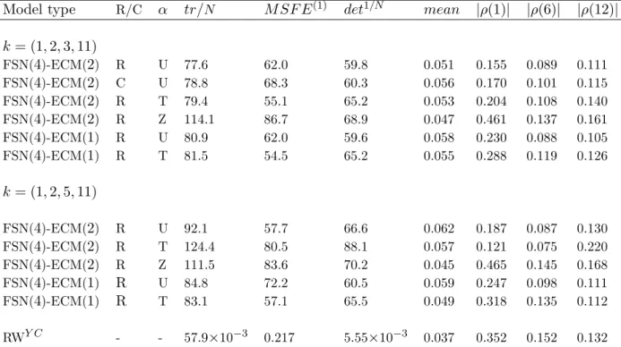
Figure 3 plots by maturity the percentage increase in MSFE relative to the RWY C (negative values thus representing superior performance compared to the RWY C_{) for the following models:}

the T-FSN(6)-ECM(2) model with triangular alpha andk= (1,2,4,18,24,84); the DNS model; and the ET forecasting equation in (12). In all cases estimation is performed recursively, except for the additional line plotted for the ET case with parameters held constant (C) throughout the forecast evaluation period. Not only does the triangular FSN(6)-ECM(2) model outperform all of the rival models (including the RWY C) at all maturities, but the percentage reductions obtained in MSFE compared to the RWY C _{are also substantial, particularly at the shorter}

maturity end of the yield curve. Considered across the entire span of maturities, the gains over the DNS model are large, with DNS performing particularly poorly and worse than the RWY C for maturities between 12 and 32 months. The Diebold and Li (2006) DNS method is the only previously published method for forecasting high dimensional yield curves. The authors report better performance for the method at forecast horizons of 6 and 12 months ahead than at the 1 month ahead horizon.

Strikingly, the ET forecasts perform worse than the RWY C for the majority of the 82 ma-turities forecast. ET forecasts produced holding the term premia parameters constant (C) have higher MSFE for all maturities than those produced using recursive estimation (R). Presumably recursive estimation improves the forecasts by enabling a degree of variation over time in the term premia, ρ(3 : 85), which are of course assumed to be time-invariant constants under the ET. The average MSFEs across the 82 maturities are 113% and 121% of that for the RWY C in the recursive and constant parameter cases respectively. It is clear from Figure 3 that the conditional mean of Theorem 1 implied by the ET is far from being the optimal MSFE predictor since the MSFEs of the T-FSN(6)-ECM(2) model are much smaller than those for either the

0 10 20 30 40 50 60 70 80 −30 −20 −10 0 10 20 maturity, τ T−FSN(6)−ECM(2) ET (R) Diebold Li (2006) ET (C)

Figure 3: Percentage reduction in model MSFEs by maturity relative to those of the RWY C.

Shown are the results for the triangular (T-) FSN(6)-ECM(2) model with k = (1,2,4,18,24,84), the Diebold and Li (2006) DNS model and the Expectations Theory (ET) forecasting equation (12). (R) stands for recursive estimation and (C) for forecasts produced using constant parameters. The horizontal axis is maturity measured in months.

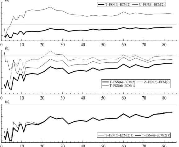
0 10 20 30 40 50 60 70 80 −25

0 25

50 (a) _{T−FSN(6)−ECM(2) U−FSN(6)−ECM(2)}

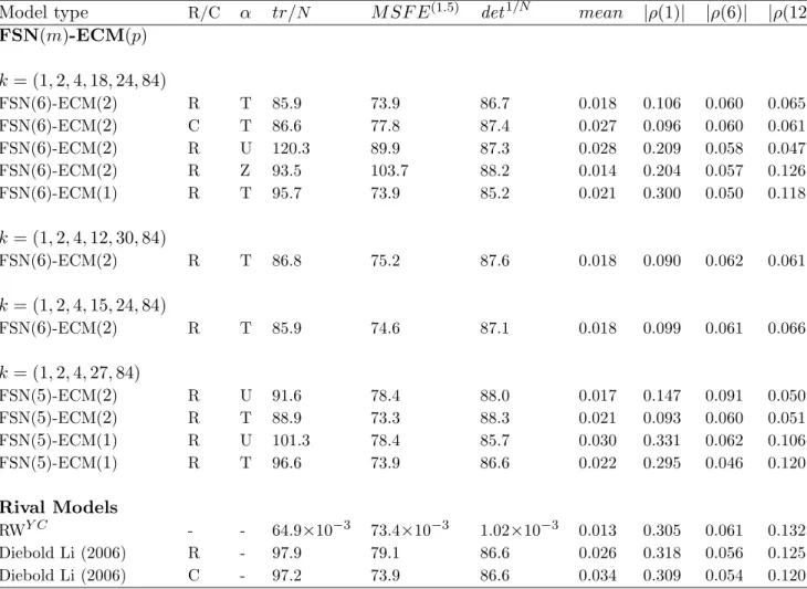
0 10 20 30 40 50 60 70 80 −30 −20 −10 0 (b) T−FSN(6)−ECM(2) T−FSN(6)−ECM(1) Z−FSN(6)−ECM(2) 0 10 20 30 40 50 60 70 80 −30 −20 −10 0 (c) T−FSN(6)−ECM(2) C T−FSN(6)−ECM(2) R

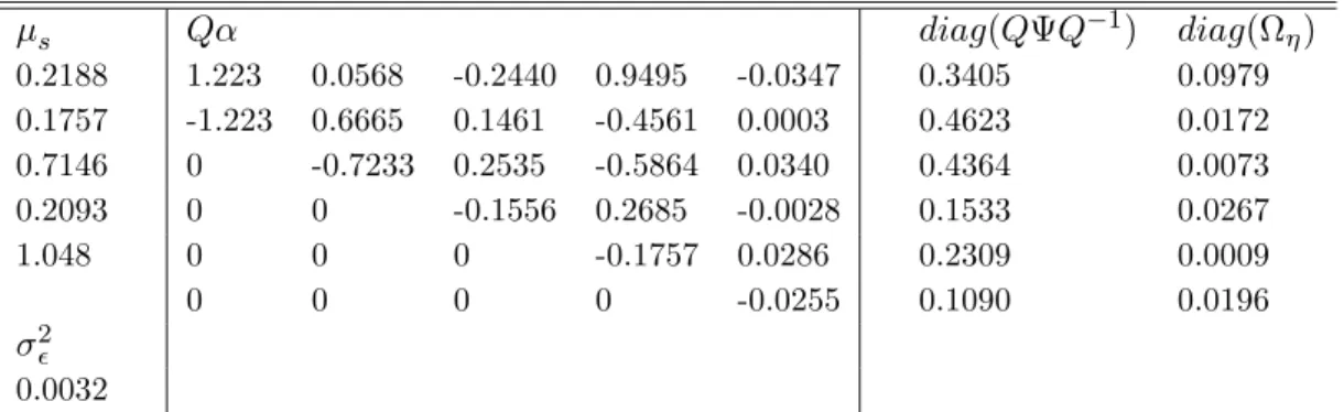
Figure 4: Percentage reduction in FSN(6)-ECM(p) model MSFEs by maturity relative to those of the RWY C. The knot vector used in all cases isk= (1,2,4,18,24,84). (a) FSN(6)-ECM(2) models with triangular (T-) and unrestricted (U-) α matrices. (b) Z- stands for a model with α = 0. (c) R stands for recursive estimation and C for forecasts produced using constant parameters. The horizontal axes are maturity measured in months.

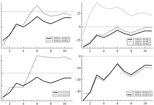
ET (R) or ET (C) cases for all maturities included. In line with this conclusion, the average across maturities of the absolute value of the first order autocorrelations of the forecast errors are 0.295 (R) and 0.288 (C), compared to a value of zero under the null that the conditional mean of Theorem 1 is the true one. The new method for evaluating the ET proposed in Section 2.2.1 thus finds that the ET is very wide of the mark. We reach the same conclusion using a differently constructed dataset consisting of the yields on a complete set of T-Bills in Section 4. Figure 4 presents analagous plots for FSN(6)-ECM(p) models, all of which havek= (1,2,4,18,

24,84) and are estimated recursively unless indicated otherwise. In each panel the T-FSN(6)-ECM(2) model of Figure 3 is shown as a thick solid line for ease of comparison. Panel (a) compares that triangular model with an otherwise identical specification in which α is

unre-stricted (U). The enormous benefit of the triangular restriction on α is clearly evident and is thought to stem from imprecise estimation of the large number of parameters in an unrestricted

α withm= 6 and time series of this length. Panel (b) highlights the impact of the restrictions Ψ = 0 and α = 0. Imposing Ψ = 0 on the ECM(2) model to obtain the T-FSN(6)-ECM(1) model is very costly in terms of MSFE for all but the shortest maturities. Imposing

α = 0 (to obtain the Z- or Zero model) is somewhat less costly for maturities greater than or equal to 7 months, but is drastically costly for the shortest maturities. Thus inclusion of the spreads β′

γ_t as regressors in the state equation (3) is crucially important for forecasting the short end of the yield curve, but also continues to play a role at the long end (witness that the line for the T-FSN(6)-ECM(2) model is still below that for the Z-FSN(6)-ECM(2) model for the longer maturities in panel (b)). It is important for forecasting (in terms of MSFEs by maturity) to retain both spreads and lagged changes in knot-yields as regressors in the ECM state equa-tion. Finally in panel (c) and for the triangular FSN(6)-ECM(2) model, recursive estimation (R) produces similar MSFEs to holding the parameters constant (C), the largest differences being for the shorter maturities and in favour there of recursive estimation. This observation suggests that parameter non-constancy is not a significant problem when forecasting the data used here with FSN-ECM models.

Table 1 reports measures of forecast performance both for the models considered in Figures 3 and 4, and for a broader range of specifications and estimation schemes. The focus is on summary MSFE-based measures, although the average across maturity of the absolute value of some sample autocorrelations of the forecast errors and of the mean forecast errors are also reported. Although the average across maturity of the MSFEs, or equivalently the trace of the MSFE matrix (denoted mM SF E), is an intuitively reasonable measure it is not invariant to non-singular linear transformations of the data even when linear predictors are used. For example, the model ordering implied by the tr(mM SF E) can in principle change when the data to be forecast is expressed as a vector consisting of the shortest rate and spreads relative to that rate, rather than as a yield curve. Also reported therefore is the determinant of the MSFE matrix, which has the desired invariance property (see Clements and Hendry 1993).13

13

To see this, let the transformed datay∗

t(τ) =P yt(τ) for some non-singularP, and denote the corresponding

MSFE matrices of the forecast errors bymM SF E∗_{andmM SF E. Provided that the forecast ˆy}∗

t(τ) =Pyˆt(τ),

then det(mM SF E∗) = det(P) det(mM SF E) det(P′). It then follows immediately that model rankings do not depend on the choice of P. Furthermore, restricting attention to cases where det(P) = 1, as is the case for

Model type R/C α tr/N M SF E(1.5) det1/N mean |ρ(1)| |ρ(6)| |ρ(12)| FSN(m)-ECM(p) k= (1,2,4,18,24,84) FSN(6)-ECM(2) R T 85.9 73.9 86.7 0.018 0.106 0.060 0.065 FSN(6)-ECM(2) C T 86.6 77.8 87.4 0.027 0.096 0.060 0.061 FSN(6)-ECM(2) R U 120.3 89.9 87.3 0.028 0.209 0.058 0.047 FSN(6)-ECM(2) R Z 93.5 103.7 88.2 0.014 0.204 0.057 0.126 FSN(6)-ECM(1) R T 95.7 73.9 85.2 0.021 0.300 0.050 0.118 k= (1,2,4,12,30,84) FSN(6)-ECM(2) R T 86.8 75.2 87.6 0.018 0.090 0.062 0.061 k= (1,2,4,15,24,84) FSN(6)-ECM(2) R T 85.9 74.6 87.1 0.018 0.099 0.061 0.066 k= (1,2,4,27,84) FSN(5)-ECM(2) R U 91.6 78.4 88.0 0.017 0.147 0.091 0.050 FSN(5)-ECM(2) R T 88.9 73.3 88.3 0.021 0.093 0.060 0.051 FSN(5)-ECM(1) R U 101.3 78.4 85.7 0.030 0.331 0.062 0.106 FSN(5)-ECM(1) R T 96.6 73.9 86.6 0.022 0.295 0.046 0.120 Rival Models RWY C - - 64.9×10−3 73.4×10−3 1.02×10−3 0.013 0.305 0.061 0.132 Diebold Li (2006) R - 97.9 79.1 86.6 0.026 0.318 0.056 0.125 Diebold Li (2006) C - 97.2 73.9 86.6 0.034 0.309 0.054 0.120

Table 1: Forecasting high dimensional yield curves: summary measures of forecast performance.

The FSN(m)-ECM(p) models are grouped according to the knot vector k; the parameter α is either unrestricted (U), triangular (T) or equal to zero (Z). The estimation procedure used is either recursive (R) or holds parameters constant at their in-sample estimates (C). The MSFE-based measures are de-noted tr/N for the average MSFE, M SF E(1.5) _{for the MSFE of the 1.5 month yield, and det}1/N _for [det(mM SF E)]1/N. With the exception of the RWY C for which the measures are reported directly, all 3 MSFE-based measures are expressed as a percentage of the corresponding measure for the RWY C_{. The} average across maturity of themeanforecast errors and of the absolute values of the sample autocorre-lations of the forecast errors at lag h,|ρ(h)|, are also reported.

The reported average MSFEs are reflective of the comments made above concerning Figures 3 and 4. Note that the average MSFE of the triangular FSN(6)-ECM(2) models is 86 to 87 per cent of that for the RWY C _{forecast, compared to 89 per cent for the triangular 5 knot}

FSN(5)-ECM(2) model and 97 to 98 per cent for the DNS model. For triangular m = 6 and m = 5 models, the average MSFE is higher for the ECM(1) models than for the ECM(2) ones. Unlike them= 6 case, the FSN(5)-ECM(2) model with an unrestricted α matrix performs quite well, presumably due to the reduction in the number of estimated model parameters.

Large reductions compared to the RWY C _{of about 25 per cent in the MSFE of the shortest}

(1.5 month) yield are achieved by all of the triangular FSN(m)-ECM(p) models withm∈ {5,6} and p ∈ {1,2}. Thus, very substantial gains over the random walk forecast of a short rate can be realised using the FSN models and the information contained in the yield curve alone. Inter-estingly, all of the models included in Table 1 perform similarly and better than the RWY C in terms of the det(mM SF E) measure, the best performer being the triangular FSN(6)-ECM(1) model. The triangular FSN(m)-ECM(2) models have substantially lower average absolute au-tocorrelations at lags of 1 and 12 months than the RWY C and DNS models.

The triangular FSN(6)-ECM(2) models (e.g. the one withk= (1,2,4,18,24,84) featured in Figures 3 and 4) are strong performers across the entire range of summary measures considered in Table 1. These T-FSN(6)-ECM(2) models dominate the rival forecasts of the RWY Cand Diebold and Li (2006) DNS methods in terms of MSFE across all maturities (recall Figure 3); have a much lower average MSFE than the DNS forecasts; achieve very large reductions in the MSFE of the short rate, conditioning on the information in past yield curves alone; and perform better than the RWY C _{and very similarly to the DNS methods in terms of the det(mM SF E) measure.}

Having considered a broad range of measures of forecast performance, we conclude that such T-FSN(6)-ECM(2) models outperform the existing methods for forecasting high dimensional yield curves.

3.5 Parameter estimates for the T-FSN(6)-ECM(2) model

We report here the QMLEs used to produce the constant parameter (C) forecasts of the trian-gular FSN(6)-ECM(2) model with k= (1,2,4,18,24,84), whose MSFEs are reported in Figure

transformation to ‘short rate and spreads’, the numerical value of the loss for a given model is also invariant to

µ_s Qα diag(QΨQ−₁ ) diag(Ωη) 0.2188 1.223 0.0568 -0.2440 0.9495 -0.0347 0.3405 0.0979 0.1757 -1.223 0.6665 0.1461 -0.4561 0.0003 0.4623 0.0172 0.7146 0 -0.7233 0.2535 -0.5864 0.0340 0.4364 0.0073 0.2093 0 0 -0.1556 0.2685 -0.0028 0.1533 0.0267 1.048 0 0 0 -0.1757 0.0286 0.2309 0.0009 0 0 0 0 -0.0255 0.1090 0.0196 σ2 ǫ 0.0032

Table 2: QMLEs of the triangular FSN(6)-ECM(2) model withk= (1,2,4,18,24,84) obtained using the training data from 1985:1 to 2000:12 inclusive as the estimation data. The operation

diag(X) gives the diagonal of the matrixX as a column vector.

4(c). This choice stems from the fact that this model specification performs well across the range of measures of forecast performance considered above, and the MSFEs for constant and recursive estimates in Figure 4(c) are very similar.

With the parameters of the state equation (3) set equal to their QMLEs, the knot-yields{γ_t} follow an I(1) process and the (m−1) spreads between them, β′

γ_t, are stationary cointegrating relations. This follows since the ranks of ˆα and ˆαβ′ are both equal to 5, the roots z of the characteristic polynomial of the VAR in (3) then satisfy either z = 1 or |z| > 1, and the determinant of [α′

⊥(I−Ψ)β⊥] is non-zero (see Johansen 1996, Theorem 4.2). The characteristic

polynomial of the VAR in (3) thus has exactly one unit root.

Table 2 reports the QMLEs of the transformed state equation (11), together with ˆσ2_ǫ. Recall that the state vector in (11) is ϕ_t = [γ_1t,(β′γ_t)′

], the vector consisting of the latent short rate and inter-knot yield spreads. The estimates of the stationary means of the spreads β′γ_t are all positive, implying that the latent yield curve is ‘upward sloping’ on average. It follows from (11) that

∆γ_1,t+1 =Qα_[1](β′γ_t−µ_s) + ∆γ_1,t+η_1t, (13) whereQα_[1]denotes the first row of the matrixQα. Bearing in mind thatk= (1,2,4,18,24,120), the estimates of the row Qα[1] in Table 2 are largest in absolute value for the spreads between the first and second, third and fourth, and fourth and fifth knot-yields. Notice that all elements of the last column ofQα are close to zero, indicating that the spread between the fifth and six knot-yields is unimportant as a regressor in (11). It also follows from (11) that the vector of

spreads follows the VAR ∆(β′ γ_t+1) =Qα_[2:6](β′ γ_t−µ_s) + (QΨQ−₁ )_[2:6]∆(β′ γ_t) +η_[2:6],t, (14) whereX_[2:6] denotes the 2nd to 6th rows of some matrix,X. With parameters set equal to the QMLEs in Table 2, this VAR is stationary. Furthermore, a given spread at (t+ 1) then depends

onlyon timetspreads involving the same and longer maturities (sinceQα_[2:6]is upper triangular and (QΨQ−₁

)_[2:6] is diagonal) and the same spread at time (t−1). Note that all elements of the estimate ofQΨQ−₁

are positive and of the estimate of the diagonal of Qα[2:6] are negative.

4

Forecasting Treasury Bill Yields

The focus of this section is on forecasting a complete set of Treasury (T-) bills with maturities ranging from 1 to 11 months inclusive. The dataset used is taken from the widely available and studied ‘Fama Treasury Bill term structure files’ contained in the CRSP monthly US Treasury database. Since zero-coupon yields on T-bills are directly observable, the analysis in this section is free of any initial method used to estimate the zero-coupon yield curve prior to analysing its dynamics. A further advantage is that the use of a yield curve dataset constructed differently to the one in Section 3 allows a check on the robustness of the findings there concerning the Expectations Theory. The results presented demonstrate the flexibility of the FSN-ECM models in forecasting different portions of the yield curve. The information set on which the forecasts are based is smaller since current and past yields with maturities greater than 11 months are excluded. Nevertheless, the use of less heavily parametrised FSN-ECM models with a smaller number of knots, m, provides an effective forecasting method in this setting. Less computation-ally burdensome models and datasets such as these are helpful when, for example, using particle filtering to form predictive densities.

The dataset is constructed by selecting for each month the T-bill closest in maturity to 12 months and then following that bill to maturity. The assumption is that the yield curve is constant over the interval between the maturity that is actually observed and the ‘target’ maturity, so the method chooses not to use linear interpolation. For a given month our dataset consists of the 11 monthly yields to maturity of T-bills,yt(1 : 11),and covers the period 1984:11

that the last 9 months of the year 2000 are omitted.14 A month is taken to equal 30.4 days when computing the yields.

The five best performing knot vectors in terms of cross-sectional fit, with m = 4 knots and first and last knots at 1 and 11 months respectively, were selected using the same in-sample procedure as that described in Section 3.3. The two internal knots of each knot vector were chosen from the set (2,3, ...,10). Only FSN(4)-ECM(p) models are considered here, again with

p ∈ {1,2}. The 2 knot vectors (1,2,3,11) and (1,2,5,11) were then carried forward to the forecast evaluation stage. The restrictions on Ωη, Ωǫ, α, and QΨQ−1 are exactly as described

in Section 3.2. As there, the Kalman filter is initialised using (γ′

1, γ ′ 0) ′ ∼(µ∗ ,Ω∗ ),where Ω∗ = 0 and µ∗

is set equal to the yields, (y0(k)′, y−₁(k)′)′, that correspond to the knot maturities and

are observed in the data for the two periods prior to our estimation period (i.e. 1984:11 and 1984:12). The estimation or ‘training data’ period is again 1985:1 to 1993:12 inclusive, and forecasts are made for each period from 1994:1 to 2000:3 inclusive.

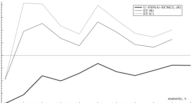
Figure 5 plots by maturity the percentage increase in MSFE relative to the RWY C _(negative

values thus representing superior performance compared to the RWY C) for the FSN(4)-ECM(2) model with unrestricted (U-) alpha and k= (1,2,3,11), and for the ET forecasts of yt(1 : 10)

from equation (6) for both recursively estimated (R) and constant (C) parameters.15 The vector of term premia, ρ₁₁, is as before estimated by OLS using the regression derived from (6), with the term premia assumed to lie on a cubic spline with knot vector (1,2,3,11) and ρ(1) = 0.

As in Section 3, the FSN-ECM model outperforms the rival RWY C and ET forecasting methods at all maturities in terms of MSFEs. The average MSFE of the U-FSN(4)-ECM(2) model is 77.6 per cent of that of the RWY C_{. The ET forecasts perform worse than the RW}Y C

for all but the 1 month yield, and ET forecasts produced holding the term premia parameters constant (C) have higher (or equal) MSFE for all maturities than those produced using recursive estimation (R). The average MSFEs across the 10 maturities are 102.3% and 109.6% of that for the RWY C in the recursive and constant parameter cases respectively. It is clear from Figure 5 that the conditional mean of Theorem 1 implied by the ET is not the optimal MSFE predictor

14

The 12 month yield and the last 9 months of the year 2000 are omitted from the dataset analysed in this section as the inclusion of either results in missing observations. Further details concerning the Fama T-Bill term structure files may be found in the CRSP monthly US Treasury database guide (pp. 29-31).

15

Comparison is not made with the Diebold and Li (2006) DNS method in this section. Since one of the dynamic factors (the ‘level factor’) of the model is equal to the limit of the latent yield curve as the maturity tends to infinity, it seems that the model is not well suited to modelling the short end of the yield curve alone.

1 2 3 4 5 6 7 8 9 10 11 −30 −20 −10 0 10 20 30 40 maturity, τ U−FSN(4)−ECM(2), (R) ET (R) ET (C)

Figure 5: Percentage reduction in model MSFEs by maturity relative to those of the RWY C.

Shown are the results for the FSN(4)-ECM(2)model with unrestricted (U-)αmatrix andk= (1,2,3,11), and for the Expectations Theory (ET) forecasting equation (6). (R) stands for recursive estimation and (C) for forecasts produced using constant parameters. The horizontal axis is maturity measured in months.

since the MSFEs of the U-FSN(4)-ECM(2) model are much smaller than those for either the ET (R) or ET (C) cases for all maturities included. In line with this conclusion, the average across maturities of the positive, first order autocorrelations of the forecast errors are 0.278 (R) and 0.281 (C), compared to a value of zero under the null that the conditional mean of Theorem 1 is the true one. As in Section 3, we find that the ET is very wide of the mark.

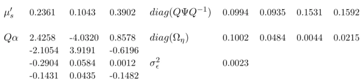
Figure 6 presents analogous plots for various FSN(4)-ECM(p) models. The models are estimated recursively unless indicated otherwise. In each panel the U-FSN(4)-ECM(2) model of Figure 5 is shown as a thick solid line for ease of comparison. Panel (a) compares that model with an otherwise identical specification in whichα is triangular (T) instead of unrestricted. In contrast to Figure 4(a), the triangular restriction results in higher MSFEs for most of the T-bill maturities. Of course the inter-knot spreads,β′

γ_t, involved are between different maturities in the two cases. Panel (b) shows the impact of imposing the restrictions Ψ = 0 or α = 0 on the U-FSN(4)-ECM(2) model. As in Figure 4(b), the α = 0 restriction is extremely costly for short maturities such as those of T-bills, supporting the earlier conclusion that inclusion of the spreads,β′γ_t,as regressors in the state equation (3) is very important for forecasting the short

2 4 6 8 10 −40 −20 0 U−FSN(4)−ECM(2) T−FSN(4)−ECM(2) 2 4 6 8 10 −25 0 25 U−FSN(4)−ECM(2) U−FSN(4)−ECM(1) Z−FSN(4)−ECM(2) 2 4 6 8 10 −40 −20 0 20 k=(1,2,3,11) k=(1,2,5,11) 2 4 6 8 10 −30 −20 −10 0 U−FSN(4)−ECM(2) C U−FSN(4)−ECM(2) R

Figure 6: Percentage reduction in FSN(4)-ECM(p) model MSFEs by maturity relative to those of the RWY C_{. (a) FSN(4)-ECM(2) models with triangular (T-) and unrestricted (U-)αmatrices, and} k= (1,2,3,11). (b) All models shown are fork= (1,2,3,11); Z- stands for a model withα= 0. (c) U-FSN(4)-ECM(2) models with the 2 different knot vectors indicated. (d) R stands for recursive estimation and C for forecasts produced using constant parameters. The horizontal axes are maturity measured in months.

Model type R/C α tr/N M SF E(1) det1/N mean |ρ(1)| |ρ(6)| |ρ(12)| k= (1,2,3,11) FSN(4)-ECM(2) R U 77.6 62.0 59.8 0.051 0.155 0.089 0.111 FSN(4)-ECM(2) C U 78.8 68.3 60.3 0.056 0.170 0.101 0.115 FSN(4)-ECM(2) R T 79.4 55.1 65.2 0.053 0.204 0.108 0.140 FSN(4)-ECM(2) R Z 114.1 86.7 68.9 0.047 0.461 0.137 0.161 FSN(4)-ECM(1) R U 80.9 62.0 59.6 0.058 0.230 0.088 0.105 FSN(4)-ECM(1) R T 81.5 54.5 65.2 0.055 0.288 0.119 0.126 k= (1,2,5,11) FSN(4)-ECM(2) R U 92.1 57.7 66.6 0.062 0.187 0.087 0.130 FSN(4)-ECM(2) R T 124.4 80.5 88.1 0.057 0.121 0.075 0.220 FSN(4)-ECM(2) R Z 111.5 83.6 70.2 0.045 0.465 0.145 0.168 FSN(4)-ECM(1) R U 84.8 72.2 60.5 0.059 0.247 0.098 0.111 FSN(4)-ECM(1) R T 83.1 57.1 65.5 0.049 0.318 0.135 0.112 RWY C - - 57.9×10−3 0.217 5.55×10−3 0.037 0.352 0.152 0.132

Table 3: Forecasting T-Bills: summary measures of forecast performance. The FSN(4)-ECM(p) models are grouped according to the knot vectork; the parameterαis either unrestricted (U), triangular (T) or equal to zero (Z). The estimation procedure used is either recursive (R) or holds parameters constant at their in-sample estimates (C). The MSFE-based measures are denotedtr/N for the average MSFE, M SF E(1) _{for the MSFE of the 1 month yield, and det}1/N _{for [det(mM SF E)]}1/N_{. With the} exception of the RWY C _{for which the measures are reported directly, all 3 MSFE-based measures are} expressed as a percentage of the corresponding measure for the RWY C_{. The average across maturity of} themeanforecast errors and of the absolute values of the sample autocorrelations of the forecast errors at lag h,|ρ(h)|, are also reported.

end of the yield curve. Panel (c) compares two U-FSN(4)-ECM(2) models withk= (1,2,3,11) and k = (1,2,5,11), with the poor performance of the latter knot vector clearly evident for maturities greater than 4 months. The knot selection procedure described in Section 3.3, whilst a very useful tool for searching over a large model space, does not ensure good forecasting performance.16 Finally, panel (d) shows that for the U-FSN(4)-ECM(2) model of Figure 5 with k = (1,2,3,11), recursive estimation produces similar MSFEs to holding the parameters constant.

Table 3 reports the summary measures of forecast performance used earlier for the two selected knot vectors and a range of model specifications, including those in Figure 6. Concen-trating on thek= (1,2,3,11) case, the U-FSN(4)-ECM(p) models achieve a very large reduction of 38 per cent in the MSFE of the 1 month yield relative to that of RWY C, whilst the

T-FSN(4)-16

One possibility not explored here would be to compare the in-sample, 1-step ahead prediction errors for selected knot vectors using the training data alone, prior to out-of-sample forecasting.