Optimal Government Debt Maturity
PRELIMINARY AND INCOMPLETE
Davide Debortoliy Ricardo Nunesz Pierre Yaredx
February 27, 2014
Abstract
This paper develops a model of optimal government debt maturity in which the govern-ment cannot issue state-contingent bonds and the governgovern-ment cannot commit to …scal policy. In contrast to an environment with full commitment, there is a tradeo¤ between the cost of funding and the bene…t of hedging. Borrowing long term provides the government with a hedging bene…t since the value of outstanding government liabilities declines when short-term interest rates rise. However, borrowing long short-term lowers …scal discipline for future governments unable to commit to policy, which leads to higher future short-term interest rates. Therefore, lack of commitment ex post increases the government’s cost of borrowing long term ex ante. A consequence of this tradeo¤ is that the slope of the yield curve is increasing in the maturity of newly issued debt. Our main theoretical result is that, as in the case of full commitment, the optimal maturity structure of government debt is tilted to the long end, but it is more ‡at than in case of full commitment. Our quantitative analysis shows that, in contrast to debt positions under full commitment–which involve a short-term asset position and a long-term debt position, both extremely large relative to GDP–debt positions under lack of commitment are positive at all maturities, much smaller relative to GDP, and have a nearly ‡at maturity.
Keywords: Public debt, optimal taxation, …scal policy, consumption and savings
JEL Classi…cation: H63, H21, E62, E21
We would like to thank participants at European University Institute, Columbia macro faculty lunch, and CREI faculty lunch for comments.
yUniversity of California, San Diego, Universitat Pompeu Fabra and Barcelona GSE: [email protected]. zBoard of Governors of the Federal Reserve System: [email protected].
1
Introduction
How should government debt maturity be structured? Two seminal papers by Angeletos (2002) and Buera and Nicolini (2004) argue that the maturity of government debt can be optimally structured so as to completely hedge the economy against shocks. Using some examples, they show that optimal debt maturity is tilted long, with the government purchasing short-term assets and selling long-term debt. This allows the market value of outstanding government liabilities to decline when short-term interest rates rise. Moreover, quantitative exercises imply that optimal government debt positions, both short and long, are large (in absolute value) relative to GDP.
In this paper, we show that these conclusions are sensitive to the assumption that the government can fully commit to …scal policy. In practice, a government chooses taxes and debt sequentially, taking into account its current portfolio of debt holdings at any date, as well as the behavior of future governments. We show that once the lack of commitment by the government is taken into account, it becomes costly for the government to use the maturity structure of debt to completely hedge the economy against shocks; there is a tradeo¤ between the cost of funding and the bene…t of hedging. Our main theoretical …nding is that the optimal maturity structure of government debt, while still tilted to the long end, is more ‡at than under full commitment. Moreover, quantitatively, the maturity structure is nearly ‡at with positive short-term and long-term debt positions which are signi…cantly smaller (in absolute value) in comparison to the case of full commitment.
We present these …ndings in the spender-saver model of Mankiw (2000).1;2 This is an en-dowment economy in which some fraction of households participate in the government bond market ("saver households") while another fraction of households do not participate in the bond market ("spender households"). Spender households experience shocks to the marginal value of their consumption and the government utilizes lump sum taxes and debt in order to smooth out their consumption. In this environment, if the government issues more bonds, these bonds are purchased by the saver households who require a higher return to be induced to purchase the bonds. Thus, a natural positive relationship between debt issuance and yields emerges.
Our model features two important frictions. First, we assume that state-contingent bonds are unavailable, and that the government can only issue non-contingent bonds of all maturities. Second, we assume that the government lacks commitment to policy, so that the government dynamically chooses its policies at every date as a function of payo¤ relevant variables: the state of the economy and its debt position at various maturities. As is well-known from previous
1We use this model of public debt as opposed to the more commonly used model of Lucas and Stokey (1983) for
technical reasons. As is shown in Krusell et al. (2006), introducing lack of commitment into the Lucas and Stokey (1983) model–even in the absence of shocks and long maturities–is complicated by the presence of discontinuities in equilibria, making quantitative analysis of the in…nite horizon economy very challenging.
2
The main results in Angeletos (2002) and Buera and Nicolini (2004)–who use the framework of Lucas and Stokey (1983)–continue to hold in the spender-saver model. Analogously, our main results continue to hold quantitatively in the environment of Lucas and Stokey (1983) in a three period economy. Details available upon request.
work, neither of these frictions on their own lead to any ine¢ ciency. First, the work of Angeletos (2002) and Buera and Nicolini (2004) shows that, even in the absence of contingent bonds, an optimally structured portfolio of non-contingent bonds can perfectly insulate the government from all shocks to the economy. Second, the work of Lucas and Stokey (1983) shows that, even in the absence of commitment by the government, an optimally structured portfolio of contingent bonds can perfectly induce a government without commitment to pursue the ex-ante optimally chosen policy ex post.
While each of these two frictions in isolation is irrelevant, the combination of the two leads to a non-trivial tradeo¤ between market completeness and commitment in the government’s choice of maturity. The more tilted is the government’s debt position towards the long end, the higher the insurance against economic shocks. However, the more ‡at the government’s debt position, the more committed the government is to its ex-ante optimal plan. To get a sense of this tradeo¤, let us consider the benchmark cases which only feature one friction.
Suppose that the government has full commitment but only has access to non-contingent bonds. In this case, the government can use the rich maturity structure of the government bonds to create insurance claims which fully insulate it from economic shocks. Speci…cally, the government’s optimal choice of maturity is tilted towards the long end, and this maturity choice guarantees that the total value of outstanding government liabilities declines whenever short-term interest rates rise and the government budget becomes tighter.
Now consider the alternate benchmark case in which the government lacks commitment, but there are no shocks, so that the government does not need to worry about insurance. In this case, the ex-ante optimal policy is perfectly smooth taxation. A government today can guarantee commitment to this policy by future governments by choosing a ‡at maturity structure, so that the lack of commitment does not impose any additional ine¢ ciency. A tilted debt position, however, would cause a future government to deviate from the optimal smooth path. If, for example, a future government chooses policy while holding only long-term debt, then it has an incentive to cut taxes and increase debt issuance ex post. This action increases ex-post short-term interest rates, which bene…ts the government by reducing the market value of its liabilities, but this hurts long-term debt holders. In contrast, if a future government chooses policy while holding only short-term debt, then it has an incentive to raise taxes and reduce debt issuance ex post. This action reduces ex-post short-term interest rates, which bene…ts the government by reducing the cost of rolling over short-term debt, but this hurts short-term debt holders. Therefore, only a ‡at maturity structure can guarantee that taxes remain smooth since the government does not have any bene…cial deviations ex post in this case (i.e., any deviation’s marginal e¤ect on the market value of long-term debt is outweighed by the marginal e¤ect on the rollover cost of short-term debt).
Our main theoretical result is that, under non-contingent bonds and lack commitment, the optimal maturity of government debt is tilted long, but is more ‡at in comparison to the case of full commitment. This result emerges from the tradeo¤ previously described above. Full
insurance with a debt position highly tilted to the long end is too expensive for the govern-ment. Suppose that the government were to choose a highly tilted debt position ex ante. Saver households purchasing government bonds ex ante would internalize the fact that ex post, the government will have lower …scal discipline and will choose lower taxes and higher debt (relative to under commitment), thereby diluting the claims of long-term debt holders. Saver households therefore require a higher yield ex ante for buying long-term debt relative to short-term debt (since short-term debt can be rolled over at higher interest rates). Therefore, borrowing primar-ily long term can be very expensive. More generally, the slope of the yield curve is increasing in the maturity of newly issued bonds, and this is because the private sector internalizes the lack of commitment by the government.3 Taking this fact into account, the government chooses a ‡atter maturity structure than under full commitment. The fact that the maturity structure is still tilted long follows from the fact that some hedging continues to be bene…cial.
We additionally provide some quantitative results. We …nd that, in contrast to the case of full commitment, under lack of commitment, the optimal maturity structure of government debt is nearly ‡at, and government debt positions at the short and long end are both positive. Furthermore, we …nd that the absolute magnitude of these debt positions are signi…cantly smaller when compared to the case of full commitment. More speci…cally, in our simulated economy, we consider an environment in which the government issues a one-year bond and a console. In our benchmark simulation, we …nd that under full commitment, the short-term bond is -124% of GDP the market value of the console is 165% of GDP, with annual payouts equal to 7% of GDP. In contrast, under lack of commitment, the short-term bond is 2.5% of GDP and the market value of the console is 61% of GDP, with annual payouts equal to 2.5% of GDP. Thus, the optimal maturity structure is essentially ‡at.
This result is intuitive and follows from the fact that completing the market–which is done under full commitment–requires very large positions relative to the size of the economy. This fact, which is also present in Angeletos (2002) and Buera and Nicolini (2004), is due to the reality that interest rates are not su¢ ciently volatile so as to allow full hedging with a small position. Such enormous positions, however, exacerbate the problem of lack of commitment, which means that such positions are extremely expensive to maintain. More generally, the cost of lack of commitment signi…cantly exceeds the bene…ts of hedging, and for this reason, optimal policy involves a nearly ‡at maturity structure.
This paper is connected to several literatures. As discussed, we build on the work of Angeletos (2002) and Buera and Nicolini (2004) by introducing lack of commitment.4 In this regard, our
3This prediction is consistent with …ndings in the empirical …nance literature (e.g., Greenwood and Vayanos,
Forthcoming). Note that this prediction is not due to the presence of segmented markets (e.g., Greenwood et al., 2010)–in our setting savers have access to debt of all maturities–but rather it is due to the lack of commitment to …scal policy.
4Additional work explores government debt maturity while continuing to maintain the assumption of full
commitment. Shin (2007) explores optimal debt maturity when there are fewer debt instruments than states. Faraglia et al. (2010) explore optimal debt maturity in environments with habits, productivity shocks, and capital. Lustig et al. (2008) explore the optimal maturity structure of government debt in an economy with nominal
work is related to that of Arellano and Ramanarayanan (2012) and Aguiar and Amador (2013), but in contrast to this work, we ignore the possibility of default and focus purely on commitment to taxation and debt issuance. Our work is also complementary to that of Arellano et al. (2013), but in contrast to this work, we ignore the presence of nominal frictions and the lack of commitment to monetary policy. In this regard, our work is most applicable to economies in which the risks of default and surprise in‡ation are not salient. Moreover, it should be noted that the absence of these risks in our framework implies that the maturity structure of government debt isnot tilted towards the short end as it is in this other work.
More broadly, our paper is also tied to the literature on optimal …scal policy which explores the role of non-contingent debt and lack of commitment. A number of papers have studied opti-mal policy under full commitment but non-contingent debt, such as Barro (1979) and Aiyagari et al. (2002).5 As in this work, we …nd that optimal taxes respond persistently to economic shocks, though in contrast to this work, this persistence is due to the lack of commitment by the government as opposed to the ruling out of long-term government bonds. Other work has stud-ied optimal policy in settings with lack of commitment, but with full insurance (e.g., Debortoli and Nunes, 2013 and Krusell et al., 2006). We depart from this work by introducing long-term debt, which in a setting with full insurance implies that the lack of commitment friction no longer introduces any ine¢ ciencies.6
Our paper proceeds as follows. In Section 2, we describe our baseline model. In Section 3, we provide our main theoretical result using a three-period example. In Section 4, we provide our main quantitative results. Section 5 concludes and the Appendix provides additional results not included in the text.
2
Model
2.1 Economic Environment
We consider an environment analogous to the spender-saver model of Mankiw (2000). Some frac-tion of households called "spenders" live hand-to-mouth so that their consumpfrac-tion equals their disposable income. Another fraction of households called "savers" participate in the government bond market and can trade government bonds of all maturities. In every period, the govern-ment issues bonds and chooses lump sum taxes applied uniformly to all households. Spender households are subject to a shock to their marginal utility of consumption. As such, the purpose of …scal policy in this framework is to e¤ectively transfer resources across household types. For example, if spenders’marginal utility of consumption is high (low), the government can reduce
rigidities.
5See also Farhi (2010) and Shin (2007). 6
Chari and Kehoe (1993a,b) and Sleet and Yeltekin (2006) also consider the lack of commitment under full insurance, though they focus on settings which allow for default. Alvarez et al. (2004) consider problems of commitment in an deterministic environment with long-term debt where the possibility of surprise in‡ation arises.
(raise) taxes to increase (decrease) spender’s consumption, and it can …nance this change in taxes by issuing more (fewer) bonds purchased by saver households.
More formally, consider an economy with discrete time periodst=f0;1; :::gand a stochastic state t 2 which follows a …rst-order Markov process. 0 is given. There is a continuum of
mass 1 of households. Mass 2(0;1)of households are spenders with preferences
E 1 X t=0 t tup(cpt), 2(0;1), (1)
wherecpt represents the consumption of spenders attandup( )is increasing and weakly concave. Spender households have a constant endowmentyp and are subject to lump sum taxes tR0, so that their consumption in every periodtsatis…es
cpt =yp t. (2)
Mass 1 of households are savers with preferences
E 1 X t=0 tur(cr t) (3)
wherecrt represents the consumption of savers andur( )is increasing and weakly concave. Saver households have a constant endowmentyr, are subject to lump sum taxes t, and can trade in the government bond market. A saver household enters every periodtwith a portfolio of bonds
n
btt+j1o1
j=0, whereb
t+j
t 1R0 represents a bond purchased att 1which matures att+j. At date
t, bondsbtt 1 mature, saver households can buy or sellt+j maturing bonds at priceqtt+j, and they choose their consumptioncrt subject to their budget constraint:
crt =yr t+ 1
X
j=1
qtt+j btt+j1 btt+j +btt 1. (4)
The government enters every period t with a portfolio of government bonds nBtt+1jo1 j=0,
whereBtt+1j R0represents a bond sold att 1which matures att+j. Following the realization of t, the government repays its immediate liabilities Btt 1, it buys or sellst+j maturing bonds
at priceqtt+j, and it chooses lump sum taxes subject to the government budget constraint:
t= 1
X
j=1
qtt+j Btt+1j Btt+j +Btt 1. (5)
the saver households, implying that for alltand t+j:
Btt+j = (1 )btt+j. (6) Equations(2),(4),(5), and (6) imply the resource constraint
cpt + (1 )crt = yp+ (1 )yr. (7) The initial level of bondsnBj11o1
j=1 is given.
It is useful to note that a key friction in this environment is the absence of state-contingent debt, since the value of outstanding debtBtt+j is independent of the realization of t+j. If state contingent bonds were available, then at any datet, the government would own a portfolio of bonds nnBtt+j1 t+j o
t+j2 t+j
o1 j=0
, where the face value of each bond payout at date t+j would depend on the realization of a history of shocks t+j 2 t+j. In our discussion, we will refer back to this complete market case.
2.2 Political Environment The government has preferences
E 1 X t=0 t tup(cpt) + (1 )E 1 X t=0 tur(cr t),
so that 2[0;1] corresponds to the relative weight that it assigns to spender households. The government cannot commit to policies. More speci…cally, in every period, nature determines
t, the government chooses policies t;
n
Btt+jo1
j=1 , and households choose their consumption
given policies and bond prices.
2.3 Markov Perfect Competitive Equilibrium
A Markov Perfect Competitive Equilibrium corresponds to a stochastic consumption and debt sequence cpt; crt; n btt+j o1 j=1 1 t=0
, a stochastic policy sequence, t;
n Btt+j o1 j=1 1 t=0 , and a sto-chastic bond price sequence
n qtt+j o1 j=1 1 t=0
. This sequence must be competitive, so that it satis…es the following conditions:
1. fcptg1t=0 is determined by the spender budget constraint (2).
2. cr t; n btt+jo1 j=1 1 t=0
maximizes saver welfare(3)subject to the saver budget constraint(4).
3. t;nBtt+jo1 j=1
1 t=0
4. (6)is satis…ed so that markets clear.
In addition, the government must optimally choose its prefered policy at every date. In this environment, government policies at any datet can be determined by backward induction. Speci…cally, at every date t, the government chooses policies as a function of the state t and the portfolio of debt
n
Btt+1j
o1
t=0 with which it enters the period. It takes into account that its
choice a¤ects future debt and thus a¤ects the policies of future governments. Saver households rationally anticipate these future policies, and their expectations are in turn re‡ected in current bond prices.
3
Three-Period Example
Given the complexity of solving for Markov Perfect Competitive Equilibrium, we focus our theoretical analysis on a simple three-period example. This example highlights the tradeo¤s between insurance and commitment which emerge in this framework. Lett = f0;1;2g and let the shock process satisfy
0 1 + ,
1 = f1 ;1 + g with equal probability, and 2 = 1
for some 2 [0;1) representing the volatility of the shock. In addition, let us assume that
= 1=2 so that groups have equal size, and that = 1so that the government only values the welfare of the spenders. Finally, let us assume thatup(cp
t) =c p
t and ur(crt) = logcrt, and that initial debt positions are zero.
In this environment, the government has …nancing needs at date 0 since spenders have high marginal utility of consumption at that date. The government can …nance these needs with short-term and with long-term debt, and in doing so, it must take into account that it faces some risk at date 1. In particular, if 1 = 1 + , it will again have some …nancing needs at date
1, and it could potentially face a rollover crisis if interest rates are high in that period.
Given that there is only a single realization of uncertainty at date 1, we refer to an allocation in this setting as , where
= ncj0; cj1( 1); cj2( 1)
o
1=1 ;1+ p;r
,
where consumption at dates 1 and 2 depend on the realization of 1.
Our main result is that there is a tradeo¤ between insurance and commitment in this frame-work and that this tradeo¤ emerges purely from the interaction between limited commitment and market incompleteness. In order to make this case, we begin by considering the two benchmark
cases of full commitment and no uncertainty. After we establish that no ine¢ ciency emerges in these two settings, we show how the interaction of the two frictions leads to a tradeo¤.
3.1 Equilibrium under Full Commitment
We begin by considering the problem of the government under full commitment. To this end, note that optimality on the side of the savers implies that bond prices must satisfy
q01= E 1 cr 1( 1) cr0,q02 = 2E 1 cr 2( 1) cr0, and q12( 1) = 1 cr 2( 1) cr1( 1) 8 1, (8)
which represent the Euler equation for all traded bonds, and whereq12( 1)represents short-term
interest rates conditional on 1’s realization. Combining constraints (4),(5), and (6) with (8),
we achieve the following conditions:
0 = y r cr 0 cr0 + E yr cr1( 1) cr1( 1) + 2E y r cr 2( 1) cr2( 1) , and (9) 0 = y r+B1 0 cr1( 1) cr1( 1) + y r+B2 0 cr2( 1) cr2( 1) 8 1 . (10)
Standard arguments (e.g., Lucas and Stokey, 1983) imply that any stochastic consumption allocation and debt policy B10; B02 which satisfy(7),(9), and(10) can be implemented as a competitive equilibrium, and that any competitive equilibrium must satisfy (7), (9), and (10). This observation allows us to use the primal approach by choosing and B01; B02 directly to maximize social welfare.
Thus, using (7) to substitute in for cpt in the government’s objective, the problem of a government with full commitment can be written as
min
;B1 0;B02
f 0cr0+ E[ 1cr1+ cr2]g s.t. (9) and (10). (11)
Proposition 1 (full commitment) Under full commitment and non-contingent bonds, the solution to(11) is crt = y r 1=2 t EhPt=0;1;2 t 1=2 t i 1 + + 2 8t, (12) B01 = yr, and (13) B02 = yr 0 @1 + E hP t=0;1;2 t 1=2 t i 1 + + 2 1 1 A, (14)
Corollary 1 (irrelevance of market incompleteness) Under full commitment, real allo-cations and welfare when bonds are state-contingent coincide with those when bonds are non-contingent.
Proposition 1 states that in the solution to the government’s problem under commitment, the level of consumption of the savers and the spenders depends only on the state of the economy t. More speci…cally, when tis high, the consumption of the spenders is also high, so that taxes are low. Therefore, at date 2, taxes are independent of the history of shocks.
Corollary 1 states that the solution to the government’s problem is the exact same as in an economy in which state-contingent bonds are available. To see why, note that under complete markets, constraint (10) can be ignored, since the debt liabilities of the government at date 1 can depend on the realization of 1, thus making (9)the only necessary constraint that must be
satis…ed so as to guarantee the satisfaction of all dynamic budget constraints of the government. Moreover, one can verify that the solution to (11) which ignores (10) also yields (12). This implies that the constraint of incomplete markets does not impose any additional ine¢ ciency in an environment with commitment.
This result is similar to that of Angeletos (2002) and Buera and Nicolini (2004), and it follows from the fact that there are as many debt maturities as the number of shocks, so that the space of uncertainty can be fully spanned. Moreover, we …nd that the types of debt positions that the government takes in order to insure itself are similar as in their work. The government takes a short asset position and a long debt position, so that the structure of government debt issuance is very tilted. The reason such a tilted debt position is optimal is that the value of the net debt position of the government declines when the spending needs of the government are high. More speci…cally, when 1 = 1 + , spending needs are high so that taxes are low and the consumption
of the spenders is high. Given that there are …nite resources, the consumption of the savers must in turn be low, so that short-term interest rates between dates 1 and 2 are high. These high interest rates imply that the price of outstanding long-term debt is low, leaving more resources for the government to spend at date 1.
Moreover, note that the quantitative magnitudes of the debt positions chosen in this stylized example can in principle be very large. For example, if the endowment of the saversyr exceeds that of the spenders yp, then the short asset position of the government B01 and the long debt positionB2
0 both exceed the total output in the economy. The observation that the debt
positions required to complete the market can be large in our simple example is consistent with the results in Angeletos (2002) and Buera and Nicolini (2004) who argue that these positions are quantitatively large–and perhaps excessively so–in a fully dynamic environment.
3.2 Equilibrium under Full Insurance
We now consider another benchmark which is the problem of the government under full insurance in an environment in which there is no government commitment. To simplify the discussion, we
let = 0 so that there is no uncertainty at date 1, and we assume at that 0 >1 so that there
are …nancing needs for the government at date 0.7
In order to solve this problem in the absence of government commitment, we utilize backward induction. GivenB01 and B02, the government at date 1 chooses policies to solve
min cr 1;cr2;B11 fcr1+ cr2g (15) s.t. 0 = y r+B1 0 cr1 cr 1 + y r+B2 0 cr2 cr 2 . (16)
where we have utilized analogous reasoning as in the construction of(11)to substitute in for the objective function and write the implementability condition(16). The solution to(15) yields
crt B01; B02 = y r+Bt 0 t 1=2 P t=1;2 t 1 1=2 t yr+B0t 1=2 1 + fort= 1;2. (17)
Now consider the problem of the government at date 0. As we previously discussed, the absence of any risk implies that constraint(10)is redundant and implied by the satisfaction of(9). Thus, the date 0 government solves
min
;fB1 0;B02g 12
f 0cr0+ E[ 1cr1+ cr2]g s.t. (9) and (17), (18)
where (17) takes into account that the government internalizes its impact on the decisions of the future government.
Proposition 2 (full insurance) In a deterministic economy with = 0 and no-commitment, the solution to(18) is crt = y r 1=2 t EhPt=0;1;2 t 1=2 t i 1 + + 2 8t and (19) B10 = B20 =yr 0 @E hP t=0;1;2 t 1=2 t i 1 + + 2 1 1 A, (20)
and constraint (17) is slack.
Corollary 2 (irrelevance of lack of commitment)In a deterministic economy, real alloca-tions and welfare when the planner has commitment coincide with those when the planner lacks commitment.
7An analogous exercise can be performed in the case in which there are shocks but state contingent bonds are
Proposition 2 characterizes the solution, and shows that it has the feature that policies are smooth from date 1 onward since there are no shocks. As stated in Corollary 2 the allocation in a deterministic economy and no commitment is identical to that under full commitment. This result is similar to that of Lucas and Stokey (1983) who show that even in an environment with no commitment, the lack of commitment imposes no additional e¢ ciency if there are as many debt instruments as there are decision-making nodes for the government. In this particular environment, one can see that a ‡at maturity structure (i.e., a maturity structure in which short debt issuance equals long debt issuance) implies that the solution under commitment can be implemented in the absence of commitment.
To gain an insight as to why a ‡at debt maturity structure provides full commitment, consider a counterfactual scenario in which all date 0 government borrowing is long, so thatB01 = 0 and B02 >0. Under full commitment, it would be possible to implement the optimum with such a maturity structure, since the government at date 1 can perfectly commit to repurchasing a …xed amount of debt and issuing a …xed amount of short-term debt so as to keep(19)satis…ed.
Under limited commitment, however, this is no longer the case, since the ex-post optimal consumption at date 1 is de…ned according to (17), which only coincides with (19) if debt is chosen optimally according to the optimal policy(20). More speci…cally, if all date 0 borrowing is long, a comparison of (17) relative to (19) given that B01 = 0 and B20 > 0 implies that the date 1 government will tilt consumption of spenders much more so into date 1 relative to date 2. Intuitively, the date 1 government prefers to deviate from the commitment solution by issuing more short-term debt than the date 0 government would prefer. The date 1 government does this since doing so increases short-term interest rates at date 1, and this happens because the increased bond issuance must be purchased by the savers who reduce their date 1 consumption relative to their date 2 consumption. This increase in interest rates translates into a reduction in the value of outstanding date 2 liabilities, which bene…ts the date 1 government. From the date 0 government’s perspective, however, this deviation is costly, since it is perfectly anticipated by the saver households at date 0 who now require a higher premium for lending long. These saver households realize that short-term interest rates at date 1 are going to be higher than anticipated under full commitment, and they therefore require a higher interest rate at date 0 to compensate them for purchasing long-term versus short-term bonds, since short-term bonds could be rolled over at date 1 at this higher interest rate.
An analogous argument holds if instead all date 0 borrowing is short, so that B01 >0 and B02 = 0. In this case, the date 1 government will tilt consumption of spenders much more so towards date 2 relative to date 1. It does this since the implied reduction in short-term debt issuance at date 1 reduces short-term interest rates at date 1, which lowers the cost of rolling over short-term debt for the date 1 government. From the date 0 government’s perspective, however, this deviation is costly, since it is perfectly anticipated by the saver households at date 0 who now require a higher premium for lending short. This e¤ect occurs because savers realize that short-term interest rates at date 1 are going to be lower than anticipated under full
commitment, and they therefore require a higher interest rate at date 0 to compensate them for short-term relative to long-term lending.
As such, a ‡at maturity structure …xes these incentive problems by making any ex-post devi-ation by the date 1 government not pro…table. More speci…cally, if the government issues more short-term debt ex post, any bene…t it achieves by diluting long-term debt is fully outweighed by the additional cost of rolling over short-term debt. Analogously, if the government issues less short-term debt ex post, any bene…t it achieves by reducing the cost of rolling over short-term debt is outweighed by the additional cost of buying back long-term debt. The private sector anticipates that the government cannot deviate ex post, and ex-ante, the ‡at maturity structure minimizes the funding costs of the government.
3.3 Equilibrium under Limited Commitment and Incomplete Markets
Propositions 1 and 2 illustrate that the constraints of non-contingent debt and no commitment by the government on their own impose no e¢ ciency loss for the economy. In the case of non-contingent debt, full insurance can be achieved by a government choosing a heavily imbalanced debt position which is tilted towards the long end. In the case of no commitment but full insurance, the current government can induce future governments to choosing its prefered policy by choosing a ‡at debt maturity structure. We now consider an environment in which the two frictions interact and we show that this leads to a tradeo¤ between insurance and commitment. As in the previous subsection, we characterize the equilibrium by backward induction. By analogous reasoning as in the construction of(15), the government at date 1 solves the following problem: min cr 1;cr2;B11 f 1cr1+ cr2g s.t. 0 = y r+B1 0 cr1 cr 1 + y r+B2 0 cr2 cr 2 ,
and the solution implies that consumption at dates 1 and 2 satisfy:
crt 1; B10; B02 = yr+B0t t 1=2P t=1;2 t 1 1=2 t yr+Bt0 1=2 1 + fort= 1;2. (21)
Substitution of the above solution into the government’s objective function implies that the expected continuation value to the government from date 1 onward can be written as
V B01; B20 = 1 1 + E 0 @X t=1;2 t 1 1=2 t yr+B0t 1=2 1 A 2 .
Moreover, substitution of(21)into(9) implies that consumption at date 0 satis…es cr0 B01; B02 = y r 1 + + 2 yr 1 + E P t=1;2 t 1 1=2 t yr+Bt0 1=2 P t=1;2 t 1 1 =2 t (yr+Bt0) 1=2 .
It thus follows that one can write period zero bond prices as a function of short debt issuance B01 and the long debt issuance B02:
q10 B01; B02 = cr0 B01; B02 E " 1 cr1 B01; B02 # and (22) q20 B01; B02 = 2cr0 B01; B02 E " 1 cr2 B01; B02 # . (23)
Using this notation, and substituting (2), (4),(5), and (6) into the government’s objective function, the date 0 problem of the government can be written as
max
B1 0;B02
0 q10 B01; B02 B01+q02 B01; B02 B02 + V B01; B02 . (24)
The …rst term in the objective function captures the bene…t at date 0 from borrowing whereas the second term captures the cost from date 1 onward of repaying the debt, taking into account the possibility of facing …nancing needs again at date 1. To get a sense of the tradeo¤s faced by the government, it is useful to see how the bond prices q10 B01; B02 and q02 B01; B02 depend on the level of bond issuance at date 0.
Lemma 1 (bond prices)q01 B01; B02 andq02 B01; B02 are continuously di¤ erentiable functions with the following properties:
1. (debt issuance and yields)q10 B01; B20 and q02 B01; B02 decrease in both B01 and B02, 2. (debt issuance and yield curve)q10 B01; B20 =q02 B01; B02 decreases inB01 and increases
in B02, and
3. (debt maturity, yields, and yield curve) q01 B01; B02 decreases and q02 B01; B02 in-creases if B01 increases andB02 decreases so as to keepcr0 B01; B02 constant.
The …rst part of Lemma 1 states that interest rates at all maturities increase in government borrowing at all maturities. To get a sense of the intuition for this result, note that from(21), the consumption of the savers at dates 1 and 2 increases with government borrowing at all maturities. This is because an increase in government borrowing represents an increase in the future wealth of savers. By constrast, this increase in consumption for savers at dates 1 and 2 implies a reduction in their consumption at date 0 according to equation (9). Intuitively,
the savers must be reducing their date 0 consumption in order to purchase the newly issued government bonds. As such, from (22) and (23), this implies that the yields at all maturities must rise.
The second part of Lemma 1 states that the slope of the yield curve, here parameterized by the ratio of the short bond price to the long bond price, is decreasing in short debt issuance and increasing in long debt issuance. In other words, although all bond prices are decreasing in debt issuance by the …rst part of the lemma, the extent to which they do so depends in part on how the maturity structure of government debt is also changing. This result builds on the fact that the private sector at date 0 prices the bonds taking into account the actions of the government at date 1. From (21), while an increase in short-term debt B01 raises savers’ consumption at dates 1 and 2, it increases date 1 consumption by more than date 2 consumption. The rationale is that the government ex post at date 1 sees a bene…t to limiting short-term debt issuance and tilting savers’ consumption towards date 1, which reduces short-term interest rates at date 1. In contrast, an increase inB2
0 raises savers’consumption at date 2 by more than at date 1. The
reason is that the government ex post at date 1 sees a bene…t to increasing short-term debt issuance and tilting savers’ consumption towards date 2, which increases short-term interest rates at date 1.
The third part of this lemma generalizes this result to a case in which the maturity structure is altered while keeping total debt issuance constant. In addition, the third part of the lemma also determines the movements in the prices of long and short-term bonds. It basically implies that, holding total borrowing …xed, a government e¤ectively changes the relative interest it pays for bonds of di¤erent maturities by altering the maturity structure. So in other words, even though issuing a more tilted maturity structure can provide more insurance, it is also more costly since it entails a much higher interest rate on long-term bonds.
To get a sense mathematically of the second and third results in Lemma 1, de…ne
= y r+B2 0 yr+B1 0 . (25)
parameterizes the maturity of the issued bonds at date 0, with higher values of denoting a longer maturity of public debt. Substitution into(22) and (23)implies that
q10 B01; B20 q20 B01; B20 = 1 1=2 E " 1=2 1 1=2 1 + 1=2 # =E " 1 1=2 1 + 1=2 # , (26)
so that the e¤ective slope of the yield curve depends only on and not on the total level of debt issuance. Moreover, one can show that that this ratio increases in .
Consider for example the government’s debt maturity in the case of full commitment de-scribed in Proposition 1. In this case, = 1 since B01 = yr, so that debt maturity is maximally tilted. If a government without commitment were to attempt this maturity
struc-ture, it would imply that q01 B10; B02 =q20 B01; B02 = 1, so that the yield curve is maximally tilted. Intuitively, saver households anticipate zero consumption and in…nite short-term interest rates at date 1, and by no arbitrage, this means that the ratio of long-term rates to short-term rates at date 0 is in…nite.
Consider instead if the government’s debt maturity were chosen to be ‡at as in the case of complete markets described in Proposition 2 with = 1. In this scenario,q01 B01; B02 =q02 B01; B02 is …nite, and with a magnitude which depends on the variance of 1. For examples, if = 0
so that there is no uncertainty regarding the value of 1, the yield curve is e¤ectively ‡at with
q01 B01; B02 =q02 B01; B02 = 1.
We now provide the main result of the paper.
Proposition 3 (limited commitment and incomplete markets) Under limited commit-ment and incomplete markets, the solution to (24) satis…es 2(1;1).
Proposition 3 states that in the presence of limited commitment and incomplete markets, the optimal debt maturity chosen by the government is tilted towards the long end, so that B02> B01, but not to the same extent as under full commitment. So in other words, the optimal maturity , is chosen to be in between that chosen under full insurance (i.e., = 1) and full commitment (i.e., =1). Intuitively, if = 1, the marginal value of hedging achieved by tilting the maturity structure towards the long end exceeds the additional marginal cost of …nancing generated by increasing the term structure of interest rates. If instead = 1, the cost of limited commitment is extremely high, since saver households anticipate immiseration at date 1, which makes short-term interest rates at date 0 to be negative in…nity and therefore implies that borrowing more short term is cheaper on the margin for the government.
4
Quantitative Exercise
In this section, we consider the quantitative implications of our model in an in…nite horizon economy. In such an economy, the government at every datetmakes a …scal policy decision as a function of the state t and the entire portfolio of outstanding bond holdings
n
Btt+1jo1
j=0. Since
the state space is in…nite, this problem is very complicated to compute. As such, we reduce the set of tradeable bonds in a manner analogous to the work of Woodford (2001) and Arellano et al. (2013). Namely, we consider an economy with two types of bonds: a one-period bond and a perpetuity with decaying coupons.8
Let bSt 1 R 0 denote the value of the one-period bond purchased by the savers at t 1. Moreover, letbLt 1 R0denote the value of the per period coupon associated with the perpetuity purchased by the savers att 1. It follows then that the budget constraint of the saver households
8None of the results of the three-period economy change if we constrain the set of tradeable bonds to a
(4)is now replaced by
crt =yr t qtSbSt +qtL bLt 1 bLt + btS 1+bLt 1 . (27)
(27)takes into account that at datet, saver households receive a ‡ow payo¤ bSt 1+bLt 1 from their portfolio of one-period bonds and perpetuities; they purchase one-period bondsbSt at price qS
t; and they exchange their non-decayed perpetuities bLt 1 for new perpetuities bLt at price qLt, where 2 (0;1] is the decay rate. The government’s budget constraint (5) is analogously replaced with
t= qtSBtS+qLt BLt 1 BLt + BtS 1+BtL1 , (28)
and the market clearing condition(6)is replaced with
BSt = (1 )bSt and BtL= (1 )bLt: (29) Note that according to this formulation, a scenario with = 0is equivalent to an economy with only one-period bonds, and a scenario with = 1 is equivalent to an economy in which consoles are available.
It is straightforward to see that in this environment, optimal portfolio allocation decisions by savers imply that the Euler equations from the three-period model(8)are now replaced with:
qSt = E " ur0 crt+1 ur0(cr t) # and qtL= E " ur0 crt+1 ur0(cr t) 1 + qtL+1 # . (30)
Moreover,(27),(28), and(29) can be combined to yield: crt =yr+
1 q
S
tBtS+qtL BtL1 BtL + BtS1+BtL1 . (31)
Note that resource constraint(7)together with(30) and(31)imply that the choice of taxes f tg1t=0 can be ignored since a stochastic sequence cpt; crt; qtS; qLt 1t=0 is uniquely pinned down
by a stochastic policy sequence fBt 1g1t=0 whereBt 1 = BtS1; BtL1 .
We assume that t=f1 + ;1 + g, withPrf t+1 = tg= . As such, analogous arguments to those of the three-period model imply that in this environment, there is generically no in-e¢ ciency due to the absence of contingent bonds if the government has full commitment. The argument is analogous to that of Angeletos (2002) and Buera and Nicolini (2004). Namely, since there are two states of the world and two securities, so the entire space of uncertainty can be spanned.
Now let us consider the case of lack of commitment and focus on an equilibrium in which the government does not commit but instead chooses policies sequentially. In a Markov Perfect Equilibrium, at every datet, the government choosesBtgiven the state( t;Bt 1), the behavior
Equi-librium consists of four functions: V ( t;Bt 1), hB( t;Bt 1), hC( t;Bt 1), and hL( t;Bt 1)
which satisfy the following conditions: 1. V( t;Bt 1) satis…es V ( t;Bt 1) = max cpt;cr t;Bt f tup(cpt) + (1 )ur(crt) + E[V ( t+1;Bt)j t]g (32) s.t. (7), (30), (31), crt+1=hC( t+1;Bt), andqLt+1 =hL( t+1;Bt). (33)
2. hB( t;Bt 1)corresponds to the value ofBtwhich maximizes the objective inV ( t;Bt 1)
givenhC( t;Bt 1) and hL( t;Bt 1).
3. hC( t;Bt 1) corresponds to the value of crt which satis…es (30) and (31) given Bt = hB( t;Bt 1),ctr+1=hC t+1; hB( t;Bt 1) , and qLt+1 =hL t+1; hB( t;Bt 1) .
4. hL( t;Bt 1) corresponds to the value of qLt which satis…es (30) given crt =hC( t;Bt 1),
crt+1 =hC t+1; hB( t;Bt 1) , and qtL+1=hL t+1; hB( t;Bt 1) .
As it holds in the three-period economy, we focus on an equilibrium with di¤erentiable policy functions. To get a sense of the Markov Perfect Equilibrium, consider a deterministic economy.9 In this case, the optimal policy under commitment requires a smooth path of consumption for spenders and savers.10 Analogous arguments to those made in our three-period example as well as in the work of Lucas and Stokey (1983) imply that in this circumstance, the optimal policy under commitment can be implemented under lack of commitment with the government issuing debt with a ‡at maturity structure.11 In our environment with a one-period bond and a long-term perpetuity, this is only possible if = 1, so that the perpetuity does not depreciate. Given this fact, and given that we are interested in looking at ine¢ ciencies which arise only from the interaction of incomplete markets and lack of commitment, we focus our quantitative exercise on the case with = 1.12
Our benchmark simulation makes the following parametric assumptions. We let = 0:96so that a period is interpreted as representing a year, with a riskless rate of 4% in a deterministic
9
We solve for the Markov Perfect Equilibrium by looking for an equilibrium in which the functions V, hB,
hC, andhLare all di¤erentiable. Our solution approach …nds a …xed point using an iteration which utilizes …rst
order conditions using these functions. We cannot prove that this Markov Perfect Equilibrium is unique, though our iterative procedures always generate the same policy functions independently of our initial guesses in the iteration.
1 0
This is always true if initial debt liabilities do not have an in…nite maturity.
1 1One can make such an argument using backward induction, using a …nite horizon economy withT periods as
T! 1.
1 2If < 1, then analogous arguments to those of Debortoli and Nunes (2013)–who analyze a deterministic
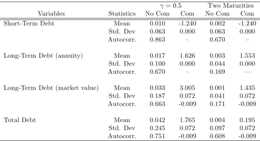
economy with a one-period bond–imply that the government debt positions are driven towards zero. In Appendix Table A-1, we provide a simulation of an economy in which = 0:5 and show that this is the case. We also provide an example with a one-period and a two-period bond and show that the same result holds.
economy. We consider CRRA preferences withup(cp) = [cp]1 p
1 =(1 p)and ur(cr) =
[cr]1 r 1 =(1 r). To start, we assume the same individual and social preferences as in the three-period model with p = 0, r = 1, and = 0. We will show that our main conclusions are robust to alternative choices of r, p, and . Based on evidence in the of Survey of Consumer Finances, we assume that = 0:4, so that 40% of households are hand to mouth and we letyp = 0:5yrso that these households have 50% of the per capital income of the saver households.13 We choose endowments so that the aggregate endowment is normalized to 1. We choose initial conditionsBS1 = 0:1625and BL1 = 0:0175 to match the maturity structure of government debt in the United States from 1988 to 2013.14 Finally, we focus on the case where shocks are i.i.d. so that = 0:5, and choose the variance of the shock process = 0:1so that our benchmark simulation generates the same standard deviation in net borrowing as in the United States over the same sample period. We perform several robustness checks to show that our results are also not driven by a particular choice for .
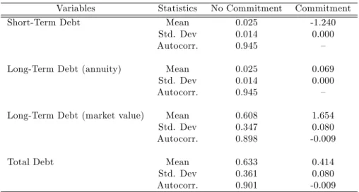
Table 1: Statistics under Baseline Parameter Values
Variables Statistics No Commitment Commitment
Short-Term Debt Mean 0.025 -1.240
Std. Dev 0.014 0.000
Autocorr. 0.945 –
Long-Term Debt (annuity) Mean 0.025 0.069
Std. Dev 0.014 0.000
Autocorr. 0.945 –
Long-Term Debt (market value) Mean 0.608 1.654
Std. Dev 0.347 0.080
Autocorr. 0.898 -0.009
Total Debt Mean 0.633 0.414
Std. Dev 0.361 0.080
Autocorr. 0.901 -0.009
Our main results from the benchmark simulation are in Table 1 where we compare various quantities in our benchmark simulation in the case of commitment to the case of no commitment. Under full commitment, in steady state, the average value of short-term bonds, BS+BL, is -124% of GDP, and the average market value of long-term bonds,qLBL, is 165% of GDP, with annuity payouts, BL, equal to 7% of GDP.15 In contrast, under lack of commitment, in steady state, the average value of short-term bonds is 2.5% of GDP, and the average market value of
1 3
We calibrate these parameters to match the percentage of families that saved and their income relative to non-savers as shown in the Survey of Consumer Finances (2012). Campbell and Mankiw (1989, 1990) and the literature discussed in Mankiw (2000) use di¤erent methodologies and …nd similar estimates.
1 4
This is done by applying a 4% discount rate to determine the value of initial annuities. These initial conditions roughly match the US statistics with a total level of debt of 60% of GDP, out of which 28% is short-term debt and 72% is long-term debt.
1 5We de…ne short-term bonds at t as representing the value of all payouts to savers due at t and long-term
long-term bonds is 61% of GDP, with annuity payouts equal to 2.5% of GDP. Thus, the optimal maturity structure is essentially ‡at.16 We …nd some additional interesting contrasting features between the two cases. In the case of full commitment, the market value of total debt essentially follows an i.i.d. process, like the underlying shock process, and this is because full insurance is possible. In contrast, under lack of commitment, the market value of total debt is persistent, and this is because the government actively manages its debt positions in response to shocks since it cannot achieve perfect insurance. Finally, note that the total value of debt is higher under no commitment versus full commitment. This follows from the fact that the optimal maturity structure is ‡at, and in this regard, having higher levels of debt allows for more insurance since the value of the net liabilities of the government then ‡uctuate more.
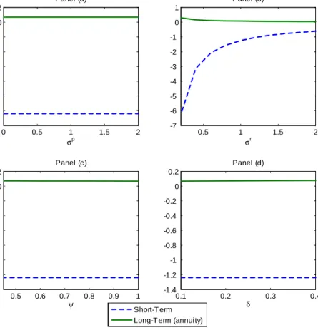
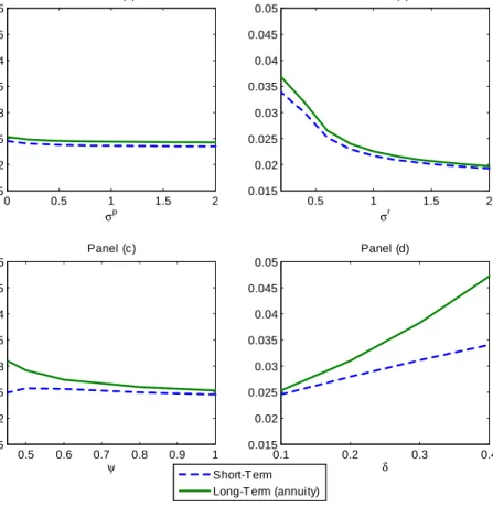
Figures 1 and 2 perform some robustness checks on our main result. Figure 1 displays the level of short-term bonds and the annuity value in the long-term bonds under full commitment. Panel (a) varies the risk aversion of the spender households p; panel (b) varies the risk aversion of the saver households r; panel (c) varies the welfare weight on the spender households ; and panel (d) varies the volatility of the shock . In all cases, the main conclusion from previous research is con…rmed: The maturity structure of government bonds is heavily tilted towards the long end and the value of debt positions are large relative to GDP. Figure 2 performs the same exercise under lack of commitment and …nds that our main conclusions are robust. In all cases, the optimal maturity structure under no commitment is close to ‡at and positions are small relative to GDP.
Figures 1 and 2 also display some interesting comparative statics. Panels (a) and (b) show that increasing the risk aversion of either the spender or saver households essentiallydecreases the need for insurance and therefore decreases the overall size of debt positions and the tilting of the maturity structure in both cases of full commitment and lack of commitment. If spender households are more risk averse, then this increases the government’s desire to smooth the spender’s consumption and therefore smooth de…cits. As a consequence, the value of the gov-ernment’s liabilities should ‡uctuate less, implying that smaller positions are required. If saver households are more risk averse, then bond prices respond more to shocks, and this implies that smaller debt positions are required to achieve insurance.
Panel (c) shows that that changing the welfare weight so that savers enter more evenly into the welfare function increases overall debt positions and the tilting of the maturity structure in both the cases of full commitment and lack of commitment. This is because in this circumstance, larger debt and higher tilting leads to a higher cost of hedging. These higher interest rates correspond to a higher level of welfare for saver households who are now weighted more heavily in the welfare program.
1 6
Our numerical analysis does suggest that the steady state distribution of the one-period bond and the console depends on the initial levels of debt. This is consistent with the case of the deterministic economy (in which the full commitment solution can be enforced) where the steady state admits zero one-period bonds and a constant level of the console which depends on initial debt. Regardless of the initial conditions the maturity structure is essentially ‡at.
Figure 1: Debt Positions –Commitment 0 0.5 1 1.5 2 -1.4 -1.2 -1 -0.8 -0.6 -0.4 -0.2 0 0.2 σp Panel (a) Short-T erm Long-T erm (annuity)
0.5 1 1.5 2 -7 -6 -5 -4 -3 -2 -1 0 1 σr Panel (b) 0.5 0.6 0.7 0.8 0.9 1 -1.4 -1.2 -1 -0.8 -0.6 -0.4 -0.2 0 0.2 ψ Panel (c) 0.1 0.2 0.3 0.4 -1.4 -1.2 -1 -0.8 -0.6 -0.4 -0.2 0 0.2 δ Panel (d)
Notes: The …gure shows short-term debt,BS+BLand long-term debt,BL, as a
function of parameters in the model with commitment. Panel (a) varies the risk aversion of the spender households p; panel (b) varies the risk aversion of the saver households r; panel (c) varies the welfare weight on the spender households
; and panel (d) varies the variance of the shock .
Panel (d) explores the impact of changing the variance of the shock process. An increase in increases the level and tilting of debt towards the long end under both cases of full commitment and lack of commitment, and this is because it increases the desire for insurance, since the bene…t of having volatile surpluses increases. In all cases, the slope of the maturity structure remains relatively ‡at.17
In sum, these numerical exercises con…rm that our conclusions from the three-period economy are robust. Debt positions under full commitment are large and heavily tilted to the long end, but this is not true under lack of commitment. Moreover, under lack of commitment, the optimal maturity structure is nearly ‡at. This result is intuitive and follows from the fact that completing the market–which is done under full commitment–requires very large positions relative to the
1 7
In the extreme case where the slope is the most tilted with = 0:4, the standard deviation of net borrowing is about 28%, while in the US data 1988-2013 it is about 3.5%.
Figure 2: Debt Positions –No Commitment 0 0.5 1 1.5 2 0.015 0.02 0.025 0.03 0.035 0.04 0.045 0.05 σp Panel (a) Short-T erm Long-T erm (annuity)
0.5 1 1.5 2 0.015 0.02 0.025 0.03 0.035 0.04 0.045 0.05 σr Panel (b) 0.5 0.6 0.7 0.8 0.9 1 0.015 0.02 0.025 0.03 0.035 0.04 0.045 0.05 ψ Panel (c) 0.1 0.2 0.3 0.4 0.015 0.02 0.025 0.03 0.035 0.04 0.045 0.05 δ Panel (d)
Notes: The …gure shows short-term debt,BS+BLand long-term debt,BL, as a
function of parameters in the model with lack of commitment. Panel (a) varies the risk aversion of the spender households p; panel (b) varies the risk aversion of the saver households r; panel (c) varies the welfare weight on the spender households
; and panel (d) varies the variance of the shock .
size of the economy. This fact, which is also present in Angeletos (2002) and Buera and Nicolini (2004), is due to the reality that interest rates are not su¢ ciently volatile so as to allow full hedging with small position. Such enormous positions, however, exacerbate the problem of lack of commitment, which means that such positions are extremely expensive to maintain. More generally, the cost of lack of commitment signi…cantly exceeds the cost of volatility, and for this reason, optimal policy involves a nearly ‡at maturity structure.18
1 8The conclusion that the welfare bene…t of smoothing economic shocks is small is more generally tied to the
5
Conclusion
The current literature on optimal government debt maturity concludes that the government should fully insulate itself from economic shocks. This full insulation is accomplished by choosing a maturity heavily tilted towards the long end with a short-term asset position and a long-term debt position, both extremely large relative to GDP. In this paper, we show that these conclusions strongly rely on the assumption of full commitment by the government. Once lack of commitment is taken into account, then full insulation from economic shocks becomes impossible; the government faces a tradeo¤ between hedging and the cost of funding. Borrowing long term provides the government with a hedging bene…t since the value of outstanding government liabilities declines when short-term interest rates rise. However, borrowing long term lowers …scal discipline for future governments unable to commit to policy, which leads to higher future short-term interest rates. We show through a series of exercises that the optimal debt maturity structure under lack of commitment–while still somewhat tilted to the long end–is nearly ‡at, with the government actively managing its debt in response to economic shocks.
While our quantitative exercise suggests that a government should be able to achieve the optimal allocation under no commitment with a ‡at maturity, it is useful to note that, in practice, government debt is often tilted towards the short end. For example, in the case of the United States, between 1988 to 2013, 28% of outstanding liabilities had a maturity below one year. A natural question concerns whether this observed behavior is simply suboptimal and can be improved by policy reform, or if this policy choice is a response to an additional friction other than lack of commitment which make it bene…cial for the government to issue more short-term bonds than long-term bonds. An interesting avenue for future research is to consider the interaction of the lack of commitment friction with additional economic frictions (such as credit frictions in …nancial markets, for example) and to explore what these frictions imply for the optimal maturity structure of government debt.
References
Aguiar, M. and M. Amador (2013). Take the Short Route: How to Repay and Restructure Sovereign Debt with Multiple Maturities. National Bureau of Economic Research, Working Paper.
Aiyagari, R., A. Marcet, T. Sargent, and J. Seppala (2002). Optimal Taxation without State-Contingent Debt. Journal of Political Economy 110(6), 1220–1254.
Alvarez, F., P. J. Kehoe, and P. A. Neumeyer (2004). The Time Consistency of Optimal Monetary and Fiscal Policies. Econometrica 72(2), 541–567.
Angeletos, G.-M. (2002). Fiscal Policy with Noncontingent Debt and the Optimal Maturity Structure. The Quarterly Journal of Economics 117(3), 1105–1131.
Arellano, C., Y. Bai, P. Kehoe, and A. Ramanarayanan (2013). Credibility and the Maturity of Government Debt. Federal Reserve Bank of Minneapolis, Manuscript.
Arellano, C. and A. Ramanarayanan (2012). Default and the Maturity Structure in Sovereign Bonds. Journal of Political Economy 120(2), 187–232.
Barro, R. J. (1979). On the Determination of the Public Debt. Journal of Political Econ-omy 87(5), 940–71.
Buera, F. and J. P. Nicolini (2004). Optimal Maturity of Government Debt without State Contingent Bonds. Journal of Monetary Economics 51(3), 531–554.
Campbell, J. and G. Mankiw (1989). Consumption, Income and Interest Rates: Reinterpreting the Time Series Evidence. In O. Blanchard and S. Fischer (Eds.), NBER Macroeconomics Annual, pp. 185–216. Cambridge, MA: MIT Press.
Campbell, J. and G. Mankiw (1990). Permanent Income, Current Income, and Consumption. Journal of Business & Economic Statistics 8(3), 265–279.
Chari, V. and P. Kehoe (1993a). Sustainable Plans and Debt.Journal of Economic Theory 61(2), 230–261.
Chari, V. and P. Kehoe (1993b). Sustainable Plans and Mutual Default. Review of Economic Studies 60(1), 175–95.
Debortoli, D. and R. Nunes (2013). Lack of Commitment and the Level of Debt. Journal of the European Economic Association 11(5), 1053–1078.
Faraglia, E., A. Marcet, and A. Scott (2010). In Search of a Theory of Debt Management. Journal of Monetary Economics 57(7), 821–836.
Farhi, E. (2010). Capital Taxation and Ownership When Markets Are Incomplete. Journal of Political Economy 118(5), 908–948.
Greenwood, R., S. Hanson, and J. C. Stein (2010). A Gap-Filling Theory of Corporate Debt Maturity Choice. Journal of Finance 65(3), 993–1028.
Greenwood, R. and D. Vayanos (Forthcoming). Bond Supply and Excess Bond Returns.Review of Financial Studies.
Krusell, P., F. Martin, and J.-V. Ríos-Rull (2006). Time-Consistent Debt. Manuscript. Lucas, R. E. (1987). Models of Business Cycles. New York. Basil Blackwell.
Lucas, R. E. and N. L. Stokey (1983). Optimal Fiscal and Monetary Policy in an Economy without Capital. Journal of Monetary Economics 12(1), 55–93.
Lustig, H., C. Sleet, and S. Yeltekin (2008). Fiscal Hedging with Nominal Assets. Journal of Monetary Economics 55(4), 710–727.
Mankiw, G. (2000). The Savers-Spenders Theory of Fiscal Policy. American Economic Re-view 90(2), 120–125.
Shin, Y. (2007). Managing the Maturity Structure of Government Debt. Journal of Monetary Economics 54(6), 1565–1571.
Sleet, C. and S. Yeltekin (2006). Optimal Taxation with Endogenously Incomplete Debt Markets. Journal of Economic Theory 127(1), 36–73.
Survey of Consumer Finances (2012). Changes in U.S. Family Finances from 2007 to 2010: Evidence from the Survey of Consumer Finances. Bulletin Board of Governors of the Federal Reserve System 98(2), 230–261.
Woodford, M. (2001). Fiscal Requirements of Price Stability. Journal of Money Credit and Banking 33, 669–728.
Appendix
A-1
Proofs
Proof of Proposition 1
Let us assume and later verify that constraint (10) does not bind. It is straightforward to show that the solution to(11) which ignores(10)admits crt which satis…es(12). One can check thatB01 andB02 which satisfy (13)and (14) satisfy(10), which veri…es that the constraint does not bind.
Proof of Proposition 2
Consider a deterministic economy with = 0. Let us assume and later verify that constraint
(17) does not bind. It is straightforward to show that the solution to (18) which ignores (17)
admits crt which satis…es (19). One can check that B01 and B02 which satisfy (20) satisfy (17), which veri…es that the constraint does not bind.
Proof of Lemma 1
We begin by proving part (i). From(21),crt 1; B01; B02 is strictly increasing in B01 and B02
fort= 1;2. This implies from(9) thatcr
0 must be strictly decreasing inB10 and B02. From (22)
and(23), this implies thatq10 B01; B20 and q02 B01; B20 are decreasing in both B01 and B20. Before proving part (ii), we prove part (iii). LetB01 increase andB02 decrease so as to keep cr
0 B01; B02 constant. From (9), it must be that either cr1 1; B01; B02 and cr2 1; B01; B02 are
both unchanged, or that one quantity increases whereas the other quantity decreases. Suppose that cr1 1; B01; B02 weakly decreases so that cr2 1; B10; B02 weakly increases conditional on 1. From (21), this would require that yr+B10 = yr+B02 weakly decreases conditional on 1, leading to a contradiction. Therefore, cr1 1; B01; B02 strictly increases and cr2 1; B01; B20
strictly decreases conditional on 1, implying from(22)and(23)thatq10 B01; B20 decreases and
q20 B01; B02 increases.
We now move to proving part (ii). Note that(21) combined with(22)and(23) implies that
q01 B01; B02 q02 B01; B02 = E " 1 cr 1 1; B01; B02 # E " 1 cr2 1; B01; B02 # = 1=2 0 B B B B @ E " 1=2 1 1=2 1 + 1=2 # E " 1 1=2 1 + 1=2 # 1 C C C C A` (A-1)
where is de…ned in (25). (A 1) implies that q1
and not on the value of cr0 B01; B20 . Suppose it were the case that q01 B01; B02 =q20 B01; B20 weakly increases if B01 increases for some B01; B02 . This would imply from (A 1) that q01 B01; B02 =q02 B01; B02 is weakly decreasing in for the associated B01; B02 (since an in-crease in B01 decreases ). However, from part (iii) proved above, starting from the associ-ated B10; B02 , any increase in B01 and decrease in B02 chosen so as to keep cr0 B01; B02 con-stant must strictly decrease q10 B01; B02 =q02 B01; B02 and decrease (by de…nition). Therefore, q10 B01; B02 =q02 B01; B02 in(A 1)cannot be weakly decreasing in for the associated B01; B02 , since this a contradiction. Analogous reasoning implies thatq01 B10; B02 =q20 B01; B02 is increas-ing inB02.
Proof of Proposition 3
Note that(24) can be rewritten as a function ofB1
0 and : min B1 0; 8 > > > < > > > : 0yr " 1 + + 2 yr 1 + 1 yr+B1 0 E 1=2 1 + 1=2 1=2 1 + 1=2 !# 1 + 1 + y r+B1 0 E 1=2 1 + 1=2 2 9 > > > = > > > ; (A-2)
which yields the following …rst order conditions:
B01 : 0[cr0]2 1 + 1 yr+B1 0 2E 1=2 1 + 1=2 1=2 1 + 1=2 ! = 1 + E 1=2 1 + 1=2 2 : 0[cr0] 2 1 + 1 yr+B1 0 2 d d E 1=2 1 + 1=2 1=2 1 + 1=2 ! = 1 + d d E 1=2 1 + 1=2 2
which imply that the optimal debt maturity necessarilly satis…es d d logE 1=2 1 + 1=2 1=2 1 + 1=2 ! = d d logE 1=2 1 + 1=2 2 . (A-3)
We …rst prove that the optimal value of does not equal 1. The value of the objective to minimize in(A 2)equals1if =1, whereas it equals a …nite number for any other positive level of . Therefore, the maximizer cannot be =1.
We now show that the solution also cannot admit 1. Suppose that this were the case. De…ne H( 1; ) = 11=2+ 1=2, F( 1; ) = 1+ 2 1=2 1 + 1=2 1=2 1 + 1=2 and G( 1; ) = 1=2 1 + 1=2 1=2 1 + 1=2
and let us expand(A 3)to achieve:
E H(1 1; ) F( 1; ) E[G( 1; )] = E[H( 1; )] E h H( 1; )2 i (A-4)
Note that sinceH( 1; ) has positive variance, one can use Jensen’s inequality to simplify the
right hand side of (A 4)to achieve:
E[H( 1; )] EhH( 1; )2 i < 1 E[H( 1; )] <E 1 H( 1; ) . (A-5)
Moving to the left hand side of (A 4), note that 1 H( 1; )
are both decreasing in 1 and
therefore have positive covariance, so that
E H(1 1; ) F( 1; ) E 1 H( 1; ) E [F( 1; )]. (A-6)
Moreover, note thatF( 1; )=G( 1; ) 1for every single realization of 1since 1, implying
that
E[F( 1; )]=E[G( 1; )] 1 (A-7)
(A 6)and (A 7)imply that
E H(1 1; ) E 1 H( 1; ) F( 1; ) E[G( 1; )] . (A-8)
A-2
Di¤erent Bond Maturities
Table A-1: Statistics with Di¤erent Bond Maturities.
= 0:5 Two Maturities
Variables Statistics No Com Com No Com Com
Short-Term Debt Mean 0.010 -1.240 0.002 -1.240
Std. Dev 0.063 0.000 0.063 0.000
Autocorr. 0.863 – 0.670 –
Long-Term Debt (annuity) Mean 0.017 1.626 0.003 1.553
Std. Dev 0.100 0.000 0.044 0.000
Autocorr. 0.670 – 0.169 —
Long-Term Debt (market value) Mean 0.033 3.005 0.001 1.435
Std. Dev 0.187 0.072 0.041 0.072
Autocorr. 0.663 -0.009 0.171 -0.009
Total Debt Mean 0.042 1.765 0.004 0.195
Std. Dev 0.245 0.072 0.097 0.072
Autocorr. 0.751 -0.009 0.608 -0.009
Notes: The table shows key statistics for alternative market structures. The …rst and second column refer to the case with a one-period bond and a long-term perpetuity with = 0:5. The third and fourth column refer to the case with a one-period bond and a two-period bond.