A Scheme of Human Face Recognition in Complex Environments

(1)

A Scheme of Human Face Recognition

in

Complex Environments

WEI CUI

A thesis submitted to Auckland University of Technology

in partial fulfilment of the requirements for the degree of

Master of Computer and Information Science (MCIS)

2014

(2)

I

Abstract

Face recognition is one of the most important biometrics in computer vision and it has been broadly employed in the area such as surveillance, information security, identification, and law enforcement. Over the last few decades a considerable number of studies have been conducted in face recognition such as Principal Component Analysis (PCA), Independent Component Analysis (ICA), Linear Discriminant Analysis (LDA), and Elastic Bunch Graph Matching (EBGM), etc. What seems to be insufficient is the research in accuracy of face recognition, it could be affected by the factors such as luminance changes, pose changes, making up, complex backgrounds, head rotation, aging issues, and emotions, etc. This thesis will limit the discussions and concentrate on accuracy problem of face recognition in complex environments.

The complex environments are considered as a place with a large number of people such as big office, internet cafés, airport, train and bus station, and casino etc. In these environments, the target human faces for recognizing usually mingle with moving objects. However, the face recognition in complex environments also can be described as the face recognition for several people who might be interested. Therefore, in this thesis, we target only the person (referred as the “Target User”) who is located closest to the camera and stationary.

In this thesis, a new scheme is proposed to recognize human faces in such complex environments. The proposed scheme can be split into three phases. The first is Moving Object Removal (MOR). The moving object could be a pedestrian, a vehicle or other moving object. The second phase is face detection which is a technology to locate a human face in a set of images or a video. The Open Source Computer Vision (OpenCV) locates human face features such as those of eyes, ears, mouth, and nose utilizing Viola-Jones algorithm. The final stage is face recognition. If a face is detected, it will be decomposed into PCA components, and then compared to other decomposed images in a face dataset.

The objective of this thesis is to propose a new scheme for human face recognition in complex environments so as to improve recognition precision and reduce false alarms. The scheme can be applied to prevent computer users against sitting too long in front of a screen.

(3)

II

Keywords: face recognition, face detection, PCA, LDA, OpenCV, digital image processing

(4)

III

List of Figures

Figure 1.1 Facial data points ... 4

Figure 1.2 Human face recognition with the assistances of eyes, nose, mouth and ears. . 4

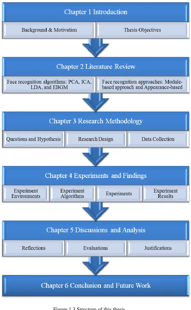
Figure 1.3 Structure of this thesis ... 7

Figure 2.1 Training procedure for a Viola-Jones based cascade classifier ... 10

Figure 2.2 Examples of Haar-like features ... 10

Figure 2.3 The calculation of the pixels in integral image ... 11

Figure 2.4 Eigenfaces ... 14

Figure 2.5 Eigenface reconstruction with various numbers of eigenvectors ... 15

Figure 2.6 The PCA based average face ... 15

Figure 2.7 The PCA workflow ... 19

Figure 2.8 Fisherfaces ... 20

Figure 2.9 Face reconstruction from fisherfaces ... 21

Figure 2.10 The LDA based average face ... 22

Figure 3.1 Two research workflows ... 35

Figure 3.2 Three main phases included in the proposed scheme ... 36

Figure 3.3 An image with high speed object and low speed object ... 37

Figure 3.4 Flowchart of the proposed scheme ... 41

Figure 3.5 Flowchart of MOR ... 42

Figure 3.6 Flowchart of face recognition ... 43

Figure 3.7 Face recognition in different environments ... 44

Figure 3.8 Face dataset ... 47

Figure 4.1 Workflow of the proposed algorithms ... 50

Figure 4.2 Face recognition in an office environment. ... 57

Figure 4.3 Face recognition in a reception environment with an insignificant moving object close to the camera ... 57

Figure 4.4 Face recognition in a reception environment with an insignificant moving object far from the camera ... 58

Figure 4.5 Face recognition in an outdoor environment ... 59

Figure 4.6 Face recognition in an outdoor environment with a truck near the camera... 60

Figure 4.7 Comparison of precisions before and after MOR ... 62

Figure 4.8 Comparison of recalls before and after MOR... 62

(7)

VI

List of Tables

Table 2.1 Comparison of PCA and LDA ... 26

Table 3.1 OpenCV cascade classifiers ... 37

Table 4.1 Numbers of frames with face recognition before and after the MOR ... 61

(8)

VII

Declaration

I hereby declare that this submission is my own work and that, to the best of my knowledge and belief, it contains no material previously published or written by another person (except where explicitly defined in the acknowledgements), nor material which to a substantial extent has been submitted for the award of any other degree or diploma of a university or other institution of higher learning.

(9)

VIII

Acknowledgements

This research completed as part of Master of Computer and Information Sciences (MCIS) course at the School of Computer and Mathematical Sciences (SCMS) in Faculty of Design and Creative Technologies (DCT) of the Auckland University of Technology (AUT) in New Zealand. I would like to thank my parents for their encouragement and support throughout my entire academic study in New Zealand. The whole school of the AUT has been extraordinary helpful in bringing this work to completion. I would like to thank all my lecturers, supervisors and administrators.

A great thank for my supervisor Dr Wei Qi Yan, he has provided supports and advices during my entire thesis time. I am not able to achieve this without his valuable support and supervision. I would also like to say thanks to my secondary supervisor Dr Kate Lee for her mathematical support.

Wei Cui Auckland, New Zealand July 2014

(10)

1

Chapter 1 Introduction

1.1

Background and Motivation

Nowadays, the requirement for reliable personal identification in access control has resulted in an increased attention in biometrics (Kocjan & Saeed, 2012; Choi et al., 2001; Jain et al., 2004; Li & Lu, 1999); it is a pattern recognition technology which operates by obtaining biometrics data from a target object (Gandhe et al., 2007), correspondingly the closest matched object will be selected from the dataset. The biometrics data can be used for machine learning and training, they are collected from the objects such as deoxyribonucleic acid (DNA), ear, gait, fingerprints, palm print, voice, iris, retina scan, signature dynamics and face (Lawrence et al., 1997; Blue et al., 1994; Burton, 1987; Qi & Hunt, 1994) for authentication and identification purpose.

Most of those biometrics data have to be collected by using special hardware such as fingerprint scanner, palm print scanner, retina scanner, DNA analyser, and the target objects have to touch with the required hardware in the stage of data collection. The face recognition does not require target object to be touched with any hardware, so as the entire face recognition is completed without awareness of the target people. Face recognition has been widely used in the area such as intelligent surveillance, information security, human identification, and law enforcement (Kondo & Yan, 1999; Chellappa et al., 1995; Vinaya & Ashwini, 2009; Pentland, 2000). Recently, face recognition has become one of the most important biometrics in computer vision (Turk & Pentland, 1991). In general, face recognition is separated into two categories: online face recognition and offline face recognition (Lawrence et al., 1997).

Online face recognition is operated by live camera, namely, face recognition will be processed synchronously while the camera is recoding. The real-time based face recognition is not only used to identify a person under live security monitoring, object tracking, civil border checking, city safety control but also is used to authenticate a person such as grant the access while deny another (for instance, access authorization to a secured building, computer, car or a gambling machine) (Pentland et al., 1993).

The offline face recognition means that face recognition will be conducted using recorded data. For example, during the investigation, a police officer could input a video

(11)

2

or an image into a face recognition system to identify suspects. The face recognition system will return a list of most suspicious ones.

A prototype having online face recognition and offline face recognition is developed for experimental purpose in this thesis. The prototype consists of two main kinds of activities, the first one is to complete face detection using the OpenCV cascade classifier and the second is recognize a face using Principal Component Analysis (PCA) algorithm (Jonsson et al., 2000).

There is a large number of face recognition algorithms having been widely studied such as PCA, LDA, ICA and EBGM (Sirovich & Kirby, 1987; Turk & Pentland, 1991; Martinez & Kak, 2001; Lu et al., 2003; Delac et al., 2005). A great deal of literatures show that automatic face analytics such as face detection, recognition and facial expression recognition are useful in recent security and forensic research (Ahonen et al., 2006; Li & Jain, 2005; Pentland et al., 1994; Wong et al., 2001). The face recognition algorithms have been proudly studied in decades (Kondo & Yan, 1999; Lee et al., 1996; Bruce & Young, 1986; Valentin et al., 1994), and a group of algorithms have been already implemented in face recognition for various purposes.

The practical applications today for human face recognition have been diffusely applied to Facebook website, cameras (Smile detection function and face detection function) amounted to a laptops and mobile phone (face unlock function), and border control system, etc. It is more noteworthy that according to the well-known Federal Bureau of Investigation (FBI) website, the FBI agency has extended its existing Integrated Automated Fingerprint Identification System (IAFIS) which criminal and civil fingerprint database was implemented to include face recognition technology (Phillips et al., 1997). The expended system is named as Next Generation Identification (NGI) and will be fully operated in summer 2014. The NGI includes FBI’s massive biometrics databases such as fingerprint database, DNA database, face database, and palm print database etc. The FBI agency also plans to collect 52 Million human face images in their NGI face database in 2015. Large scale of image collection for face recognition includes both non-criminal and criminal people’s photos.

Recently, the FBI face recognition system has been applied to the area of combating passport fraud, supporting law enforcement, identifying missing children and minimizing benefit/identity fraud (Phillips et al., 1997). Also, authentications of driver’s licenses and photo ID were used by other authorized government (Chellappa et al.,

(12)

3

1995). In addition, most of international airports have implemented the face recognition system for border check, such as the “SmartGate” system which is used to match the passport holder’s face with their passport photo in New Zealand, Australia and Singapore etc. If a passport holder could not be identified by the system, the system will then send an alarm to the nearest custom officers.

Moreover, a face recognition system has been introduced to casino which could help security to identify the problem gamblers. For instance, when a problem gambler walks in and sits in front of a pokie machine, a camera mounted in the pokie machine is used to capture the gambler’s face, the captured image will be compared to the trained face images in the existing human face database so as to identify if this is a problem gambler. The pokie machine will lock out the gamblers if the face recognition system identified them.

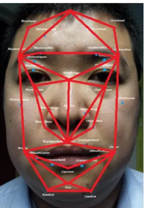
However, as one of the digital image processing and object recognition problems, face recognition still suffers from problems such as luminance changes (Choi et al., 2001), pose changes, mark-up (facial data points change in Figure 1.1), complex background, head rotation, aging issues, and expressions etc (Ahonen et al., 2006; Goldstei et al., 1971; Grudin, 2000; Lu et al., 2003; Maio and Maltoni, 2000). Most of these problems are still under investigation.

In Figure 1.1, the facial data points include the 35 points indicated the different parts of a human face such as eyebrows, right mid eyebrows, left mid eyebrows, nose bridge, nose tip, right lip upper bend, left lip upper bend etc., respectively.

(13)

4

Figure 1.1 Facial data points

Therefore, in border control, a passport holder is usually identified by the officer using the information of eyes, nose and mouth provided by the passport photo. Sometimes, earmark also has to be taken into consideration as the complementary information since human ears have been changed seldomly which are not affected by any plastic surgeries. As shown in Figure 1.2, the OpenCV face detection identifies a person’s face and ears using the information marked by red rectangles.

(a) (b) (c)

Figure 1.2 Human face recognition with the assistances of eyes, nose, mouth and ears.

(14)

5

In this thesis, a new scheme for face recognition in complex environments is proposed. In order to correctly count elapsed time and reduce false alarms in complex environments, the frame difference has been applied to detect motions and remove the moving objects from the background of motion pictures so as to increase face recognition precision.

1.2

Objectives of This Thesis

As mentioned in Section 1.1, the accuracy of human face recognition has always been the major concern for most of the security systems, identification systems and border check systems. In the past few decades a considerable number of studies have been made on the face recognition algorithms such as PCA, LDA, ICA, and EBGM. The understanding of those algorithms has been awarded, the face recognition approaches such as feature-based approaches and appearance-based approaches have been investigated as well.

A new scheme of human face recognition in complex environments has been developed in this thesis, to increase the precision and recall of face recognition is the main mission of this thesis. To achieve this goal, both theory and practice of face recognition have been studied. Theoretically, we have studied the algorithms of face detection and recognition; meanwhile we also developed a face detection and recognition prototype with MOR in practice.

1.3

Structure of This Thesis

The structure of this thesis is shown in Figure 1.3 below. This thesis consists of three main folds: understanding and planning, designing, implementation, testing and evaluation.

In Chapter 2, the literature review of face detection, face recognition and MOR are studied. The chapter covers detail understanding of various face recognition algorithms and approaches. The understanding of the OpenCV cascade classifier, Moving Object Detection (MOD) and MOR are also mentioned in this chapter.

In Chapter 3, the research methodology of this thesis is explained. The main hypotheses are tested as well as the main issues and potential solutions to the problems are explained. The experimental layout and design, dataset and implementation are depicted finally.

(15)

6

In Chapter 4, the experimental results and main outcomes are demonstrated. The chapter introduces the experimental test bed and analysis of experimental results. The outcomes of the experiments are detailed with the supports of tables and figures.

In Chapter 5, the analysis and discussions are presented based on the experimented outcomes and results. The main research hypotheses are tested and analysed with the final experiment results. The limitations of this research will be discussed as well. The conclusion and future work will then be presented in Chapter 6.

(16)

7

(17)

8

Chapter 2 Literature Review

To achieve our objectives, three important research areas are expected to be studied. The first area is face detection, the second is face recognition and the third is Moving Object Removal (MOR). In this thesis, face detection was conducted by using OpenCV cascade classifier while face recognition was developed by using Principal Component Analysis (PCA) algorithm, moreover the MOR was implemented by using frame differencing.

In this chapter, a detailed understanding of OpenCV cascaded classifier will be discussed, followed by analysis of the most popular face recognition algorithms, for instance, PCA, ICA, LDA, and EBGM, as well as two important face recognition approaches, namely, appearance-based approach and module-based approach. The MOR sample frames will be presented in the last section.

(18)

9

2.1 Introduction

The main objectives of this chapter are to explain and evaluate the research studies that are related to face detection, face recognition and MOR. By addressing the recent studies and research backgrounds, this chapter presents an important understanding of literature review. This research aimed at finding a solution which improves precision of human face recognition in complex environments and the suggested solutions will be given.

In this chapter, literature review achieves an overall understanding of face detection, face recognition and MOR. In Section 2.2 a detailed understanding of the face detection will be presented, Section 2.3 as overall understanding of face recognition will be described, and it will be followed by detailed review of the most popular face recognition algorithms and approaches in Section 2.4 and 2.5. The evaluations and comparisons of the studied face recognition algorithms will be presented in Section 2.6 and the MOR is analysed in Section 2.7.

2.2 Face Detection

Face detection is a compulsory stage in face recognition. In this thesis, the OpenCV cascade classifier is used for face detection, it is one of the most popular classifications, it was proposed by Paul Viola and Michael J. Jones in 2001 known as Viola-Jones object detection framework (Viola & Jones, 2001).

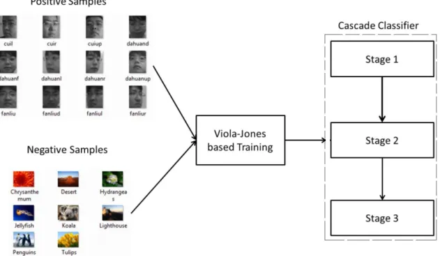
The cascade classifier means that the subsequent classifier consists of several simpler stages (Castrillon et al., 2011). As shown in Figure 2.1 these stages are applied to a region of interest until the input samples are rejected or accepted.

(19)

10

Figure 2.1 Training procedure for a Viola-Jones based cascade classifier

Haar-like features as shown in Figure 2.2 are adjacent rectangular regions that applied to a specific location in an image, and summed up the pixel intensities in each region and calculated the difference between these sums (Viola & Jones, 2001).

Figure 2.2 Examples of Haar-like features

(a)

(b)

(20)

11

As shown in Figure 2.2, (a) and (b) are represented as a two-rectangle feature, (c) is used to show a three-rectangle feature and (d) is described as a four-rectangle feature. The sum of the pixels in white rectangles is subtracted from the sum of the pixels in the black rectangles. For instance, the calculation result of two-rectangle feature such as (a) and (b) is the difference between the sum of the pixels within white rectangular area and black rectangular area. Both white rectangular area and the black rectangular area have the same size. The three-rectangle feature calculates the sum of the image pixels in white rectangle area subtracted from the sum of the image pixels in a black rectangle area. The four-rectangle feature calculates the difference between both white rectangle area and both black rectangle area (diagonal pair) (Viola & Jones, 2001; Papageorgiou et al., 1998).

However, the Haar feature detection framework is with the help of rectangular area, the computing speed is relatively slow. To increase the computing speed, an intermediate representation for the image is used, namely, Integral Image (Viola & Jones, 2001).

The Integral Image at point (x, y) contains the sum of intensities to the above this point (x, y) and to the left this point (x, y) shown in equation (2.1).

𝑖𝐼𝑚𝑎𝑔𝑒(𝑥, 𝑦) = ∑_𝑥,_≤𝑥,𝑦,_≤𝑦𝑖(𝑥,, 𝑦,) (2.1)

where 𝑖𝐼𝑚𝑎𝑔𝑒(𝑥, 𝑦) is the integrated image point (x, y), and 𝑖(𝑥,_{, 𝑦},₎_{is the original}

image.

(21)

12

In Figure 2.3, the value of the integral image at point (𝒙_𝟏,𝒚_𝟏) is the total of the pixels in rectangle A. The value at pixel (𝒙_𝟐,𝒚_𝟐) is A + B. The value at pixel (𝒙_𝟑,𝒚_𝟑) is A + C. The value at pixel (𝒙_𝟒,𝒚_𝟒) is A + B + C + D.

By using the integral image as image representation, the rectangular features can be computed rapidly. It follows that any two-rectangle feature can be computed in six array references such as arrPoint1 (𝑥0,𝑦0), arrPoint2 (𝑥1,𝑦0), arrPoint3 (𝑥0,𝑦1), arrPoint4

(𝑥₁,𝑦₁), arrPoint5 (𝑥₂,𝑦₀), and arrPoint6 (𝑥₂,𝑦₂). The same logic could be applied to three-rectangle feature which can be computed in eight array preference, and any four-rectangle feature can be calculated in nine array preference etc.

2.3 Face Recognition

In the past few decades a considerable number of studies have been made on automatic face recognition algorithms such as PCA (Turk & Pentland, 1991), ICA (Bartlett, 200), LDA (Zhao et al., 1998), Evolutionary Pursuit (EP) (Liu & Wechsler, 2000), EBGM (Wiskott et al., 1997), Kernel Methods (Yang, 2002; Lu et al., 2003), Trace Transform (Kadyrov & Petrou, 2001; Srisuk et al., 2003), Active Appearance Model (AAM) (Cootes et al., 2002), 3D Morphable Model (Blanz & Vetter, 2003), 3D Face Recognition (Bronstein et al., 2004), Bayesian Framework (Liu & Wechsler, 1998), Support Vector Machine (SVM) (Guo et al., 2000), Hidden Markov Models (HMM) (Nefian & Hayes, 1999), and Boosting & Ensemble Solutions (Lu et al., 2006).

Over the past few decades a considerable number of researches have been made on face recognition, they focus on the comparisons of face recognition accuracy (Yang et al., 2004; Draper et al., 2003; Martinez & Kak, 2001; Hanmandlu et al., 2013; Delac et al., 2005; Belhumeur et al., 1997). However, some other researchers addressed the disagreements of the comparing results. There are three main factors caused the different outcomes. The first factor is experiment environments, the second is the face databases such as FERET Database, Yale face database and AT&T face database etc., and the third factor is the experiment methods. For instance, Belhumeur et al., present the comparison result for both PCA and LDA, claim that the PCA algorithm has more error than the LDA algorithm, also the PCA algorithm is more sensitive with the lighting than that of LDA algorithm. But the PCA algorithm is insensitive to small or gradual changes on the face (Belhumeur et al., 1997; Slavkovic and Jevtic, 2012) Draper et al., concluded the comparison for PCA and ICA indicated that the ICA-I performed better than PCA-L2, but the PCA-L2 performed better than the ICA-II and

(22)

13

the PCA-L1 (Draper et al., 2003). However, the researchers Yang et al. presented a different view; that the 2D PCA performs better than that of PCA and ICA. Moreover the PCA and ICA have the same performance result (Yang et al., 2004). Martinez and Kak stated that the PCA algorithm outperforms the LDA algorithm (Martinez & Kak, 2001). Hiremath and Mayakar presented that in a constrained environment, the PCA algorithm is faster and simpler compare with LDA algorithm (Hiremath & Mayakar, 2009; Slavkovic and Jevtic, 2012). As a result, it is impossible to conclude the best algorithm for face recognition. The selection of the algorithm completely depends on the purpose.

The PCA was applied by Kirby and Sirovich to face images that is an optimal compression scheme which minimizes the mean squared error between the original images and their reconstructions for any given level of compression (Sirovich and Kirby, 1987; Turk and Pentland, 1991; Draper et al., 2003). The LDA is a statistical approach for classifying samples of unknown classes based on training samples with known classes. The ICA minimizes both second-order and higher-order dependencies in the input data and attempts to find the basis along which the data are statistically independent (Delac et al., 2005). The EBGM consists of a group of nodes that located at fiducial points and edges between the nodes as well as connections between nodes of different poses are defined (Wiskott et al., 1997). The SVM is learning algorithm that analyses data and recognize patterns, and it is used for classification. It was developed by V. Vapnik (Osuna et al., 1997). The embedded Hidden Markov Model (HMM) is using a 2D Discrete Cosine Transform (DCT) feature vector as the reflection vector to recognize the faces detected (Chen et al., 2010). Most current face recognition techniques refer to the appearance-based recognition work since late 1980’s (Draper et al., 2003).

2.4 Facial Recognition Algorithms

2.4.1 Principal Component Analysis (PCA)

Recently, one of the best algorithms on frontal face recognition is PCA. The PCA is a statistical dimensionality-reduction approach where face images are stated as a subset of their eigenvectors and eigenvalues. In other words, it turns out the best possible linear least-squares decomposition of a training set (Sirovich and Kirby, 1987; Turk and Pentland, 1991; Graham and Allision, 1998; Martinez, 2000; Moghaddam & Pentland, 1997; Gottumukkal & Asari, 2004; Moon & Phillips, 2001).

(23)

14

In addition, the PCA is an optimal compression scheme that minimizes the mean squared error between the original images and their reconstructions for any given level of compression. Turk and Pentland used PCA to compute a set of subspace basis vectors also called eigenfaces shown in Figure 2.4 for a face database (Turk & Pentland, 1991). The projected face images (mug shot) from the face dataset into the compressed subspace is known as eigenspace. The subspace crossed by the principal directions are identical to the cluster centroid-based subspace specified by the between-class scatter matrix. To recognize a face, the input test image will be decomposed, then the input face will be used to match face images in the face dataset by projecting them onto the basis vectors and then finding the nearest compressed face image in the subspace (Draper et al., 2003).

In eigenfaces method, jet colormap is presented in Figure 2.4. There are three important information we can read from the jet colormap based eigenfaces. The first information is face features (eyes, nose, and mouth in eigenfaces 8). The second information is greyscale values. And the last information is illumination in the images (Left lighting in eigenface 2).

eigenface 1 eigenface 2 eigenface 3 eigenface 4 eigenface 5

eigenface 6 eigenface 7 eigenface 8 eigenface 9 eigenface 10 Figure 2.4 Eigenfaces

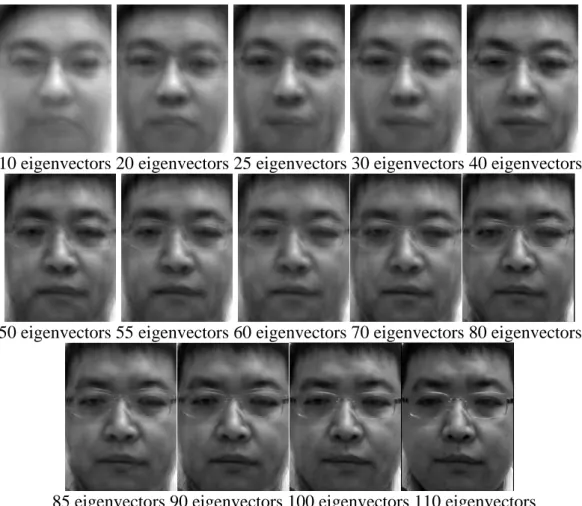
The eigenface is not visible to human, the face reconstruction is a way to reconstruct human face from eigenfaces to a visual one. The determination of how many eigenvectors are required to process the face reconstruction depends on face dataset. As

(24)

15

shown in Figure 2.5, the most important face features are already recovered with 50 eigenvectors. The eigenfaces could be recovered completely with 110 eigenvectors.

10 eigenvectors 20 eigenvectors 25 eigenvectors 30 eigenvectors 40 eigenvectors

50 eigenvectors 55 eigenvectors 60 eigenvectors 70 eigenvectors 80 eigenvectors

85 eigenvectors 90 eigenvectors 100 eigenvectors 110 eigenvectors Figure 2.5 Eigenface reconstruction with various numbers of eigenvectors

The average face as shown in Figure 2.6 is the average of training images, it is used to get the mean-subtracted images. For example, an image set X has N images 𝑥_𝑖 (𝑖 = 1, … , 𝑛) such as 𝑋 = {𝑥₁, 𝑥₂, 𝑥₃, … 𝑥_𝑁} , 𝑋̅ is average face of the training images.

(25)

16

The relationship between eigenvectors and eigenvalues in a given matrix A is shown

in equation (2.2),

𝐴𝑋= 𝜆X (2.2)

where λ is the eigenvalue and X is the eigenvector of the matrix A.

By using equation (2.2), we can generate equations (2.3) and (2.4),

𝑨𝒙 − 𝝀𝒙 = 𝟎 (2.3)

(𝐴 − 𝜆𝐼)𝑥 = 0 (2.4)

where A is the n × n matrix, I is the n × n identity matrix.

Covariance is to measure two or more matrixes which are same or not. The PCA finds the optimal linear least-squares representation shown in equation (2.5),

𝑐𝑜𝑣(𝑋, 𝑌) =∑𝑛𝑖=1(𝑋𝑖−𝑋̅)(𝑌𝑖−𝑌̅)

(𝑛−1) (2.5)

where X and Y are the vectors, 𝑋̅ and 𝑌̅ are their means respectively.

A n×n image 𝑥_𝑖 is represented by,

𝑋 = {𝑥₁, 𝑥₂, 𝑥₃, … , 𝑥_𝑛} (2.6) where X is a collection of image set.

To find patterns by using PCA for a set of images, an image matrix (iMatrix) could

be created by putting all the image vectors (iVector) together. Because each image vector is 𝑛2_{-dimension, so it has}_𝑛2 _iVectors_{which is shown in (2.7):}

𝑖𝑀𝑎𝑡𝑟𝑖𝑥 = ( 𝑖𝑉𝑒𝑐𝑡𝑜𝑟 1 𝑖𝑉𝑒𝑐𝑡𝑜𝑟 2 𝑖𝑉𝑒𝑐𝑡𝑜𝑟 3 𝑖𝑉𝑒𝑐𝑡𝑜𝑟 4 . . . 𝑖𝑉𝑒𝑐𝑡𝑜𝑟 𝑛) (2.7)

where iVector is the image vector and iMatrix is the image vector matrix which consists

of n eigenvectors.

In 1991, Matthew and Alex implemented a formula as shown in equation (2.8) for the image training set of face images 𝑥₁…𝑥_𝑛(Turk & Pentland, 1991),

(26)

17 𝐶𝑜𝑣 = 1 𝑛∑ Ф𝑖Ф𝑖 𝑇 𝑛 𝑖=1 (2.8)

where Ф_𝑖 is eigenvector represented by (𝑋_𝑖 − 𝑋̅) and (𝑌_𝑖 − 𝑌̅) from equation (2.5), n is the number of images in the training set.

(2.9) and (2.10) are used to calculate the image covariance matrix,

𝑆_𝑇 = ∑𝑛𝑖=1(𝑥𝑖 − 𝜇)(𝑥𝑖 − 𝜇)𝑇 (2.9) 𝐺𝑇 = 1 𝑛∑ (𝐴𝑗 − 𝐴̅) 𝑇_(𝐴 𝑗− 𝐴̅) 𝑛 𝑗=1 (2.10)

where 𝑆_𝑇 and 𝐺_𝑇 are the covariance matrices, 𝜇 and 𝐴 are the mean of the image training set 𝑥_𝑖 and 𝐴_𝑗.

Taken the equation (2.8) into consideration, we produce the equation (2.11),

𝐶𝑜𝑣 = 𝐴𝐴𝑇 (2.11)

where A is the matrix A = [Ф1, Ф2, Ф3, ⋯ , Ф𝑛].

To calculate the eigenvectors and eigenvalues, we need to use a computationally feasible method to find these eigenvectors which as shown in (2.12). Assume that the eigenvectors 𝑣_𝑖 of 𝐴𝐴𝑇_{, therefore,}

𝐴𝐴𝑇_𝑣

𝑖 = 𝜇𝑖𝑣𝑖 (2.12)

where 𝑣_𝑖 is eigenvectors and 𝜇_𝑖 is eigenvalues.

Following these analysis, we construct the n × n matrix MA =𝐴𝐴𝑇, where 𝑀𝐴𝑛𝑛 =

Ф_𝑛Ф_𝑛𝑇, and find the n eigenvectors 𝑉_𝑖 of matrix MA. Those vectors determine linear

combinations of the MA training images to the eigenfaces 𝐸_𝑖 as shown in equation

(2.13),

𝐸_𝐼 = ∑𝑛_𝑘=1𝑣_𝑖𝑘Ф_𝑘 (2.13)

where eigenfaces 𝐸_𝑖 and 𝑖 = 1, 2, 3, ⋯ , 𝑛

Once a new face image I is projected into eigenface, and the weight can calculate in

equation (2.14)

(27)

18

where k = 1, 2, 3, … n. The weight from a projection vector is shown in equation (2.15),

ΩT _{= [W}

1, W2, W3, ⋯ , Wn] (2.15)

Equation (2.15) describes the contribution of each eigenface in representing the input face image, treating the eigenfaces as a basis set for face images. The projection vector is then used in a standard pattern recognition algorithm to identify which of a predefined face classes, if any, best describes the face. The face class 𝛺_𝑘 can be calculated by averaging the results of the eigenface representation over a small number of face images of each individual. Classification is performed by comparing the projection vectors of the training face images with the projection vector of the input face image. This comparison is based on to find the closest square distance (Euclidean Distance) between the PCA subspace classes from face database and the PCA subspace class from the input face image as shown in equation (2.16). The Euclidean Distance classification is a decision rule which is based on the Euclidean distance between the sample projections class Ω and the projection of the k-th class mean 𝛺_𝑘,

𝜀_𝑘 = ‖(Ω − Ω_k)‖ < ∆ (2.16)

where 𝜀_𝑘 represents Euclidean Distance, 𝛺_𝑘 is a vector described the 𝐾𝑡ℎ_{faces class. If}

the Euclidean Distance is less than ∆ (Threshold Value), then the new face is classified to class k.

The eigenvector can be calculated efficiently using Singular-Value Decomposition (SVD) and they are statistically determined by covariance matrix. The third module is to identify the face in a normalized image (Moon & Phillips, 2001). However, the PCA could only capture the invariance with the limitation of the information provided in the training data.

In Figure 2.7, the overall workflow of how face recognition works via using PCA algorithm. There are two pathways to be considered. The first pathway starts from input image, which means this image will be used for recognition purpose. The second pathway starts from face database, where all the source faces are stored and trained. The recognition process is to find out which image in the face database matching with the input image. The decision making of matching or not matching will be based on the Euclidean Distance between the testing class and the training class.

(28)

19 Face Database Input Image Projection of input image Training Set PCA (Feature Extraction) PCA (Feature Extraction)

Image Vectors Image Vectors

Compare the classes and find the nearest (Euclidean Distance)

Decision Making

Not Match Match

Figure 2.7 The PCA workflow

2.4.2 Independent Component Analysis (ICA)

Independent Component Analysis (ICA) is a PCA related method (Yang et al., 2004). ICA has the following potential advantages over PCA: (1) ICA provides a better

probabilistic model of the data that identifies where the data focus in n-dimensional. (2)

It uniquely identifies the mixing matrix. (3) It may rebuild the data better than PCA in the presence of noise by finding an unnecessary orthogonal basis. (4) It not only focus on the covariance matrix but also sensitive to high order (third order) statistics in data (Bartlett et al., 2002). Bartlett and Draper proposed using ICA for face recognition and found that ICA can perform remarkable result if the Euclidean distance is used. Liu and Wechsler also state that the ICA has the power to solve the problem of unknown source

(29)

20

separation. However, the computational time in ICA is longer than PCA (Liu & Wechsler 1999; Comon 1994; Hyvarinen & Oja 1997; Karhunen et al., 1997).

2.4.3 Linear Discriminant Analysis (LDA)

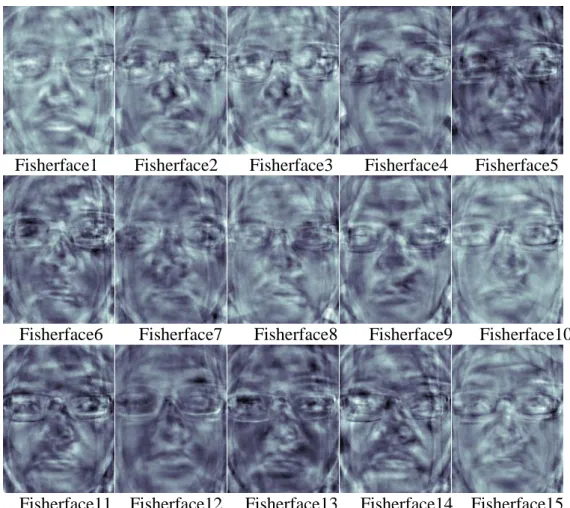
Linear Discriminant Analysis (LDA) which is known as Fisher Discriminant Analysis (FDA) as shown in Figure 2.8 (Martinez & Kak, 2001) was proposed to find the most discriminating features in the face classes (Hanmandlu et al., 2013). It is considered as one of the most successful algorithms in Face Recognition (Lu et al., 2003; Yu and Yang, 2001).

Because the Fisherfaces method does not capture the illumination as the eigenfaces does, therefore, the Fisherfaces have no chance to learn the illumination. As a result, if the Fisherfaces method was trained from an input image which was taken in a good lighting condition, then the method will find the wrong components with the recognized faces in bad lighting condition.

Fisherface1 Fisherface2 Fisherface3 Fisherface4 Fisherface5

(30)

21

The Fisherfaces also allow face reconstruction by using Fisherface method which is shown in Figure 2.9. However, they are not good as the eigenface reconstruction does. There is no expectation of a nice reconstruction to original face.

Reconstruction from Fisherfaces 1 Reconstruction from Fisherfaces 2 Reconstruction from Fisherfaces 3 Reconstruction from Fisherfaces 4 Reconstruction from Fisherfaces 5 Reconstruction from Fisherfaces 6 Reconstruction from Fisherfaces 7 Reconstruction from Fisherfaces 8 Reconstruction from Fisherfaces 9 Reconstruction from Fisherfaces 10 Reconstruction from Fisherfaces 11 Reconstruction from Fisherfaces 12 Reconstruction from Fisherfaces 13 Reconstruction from Fisherfaces 14 Reconstruction from Fisherfaces 15

Figure 2.9 Face reconstruction from fisherfaces

(31)

22

Figure 2.10 The LDA based average face

Fis h

There are two methods defined in LDA. Between-class scatter matrix (𝑆_𝐵) represents

the scatter of features around the overall mean for all face classes shown in equation (2.17),

𝑆_𝐵 = ∑𝑐_𝑗=1𝑁_𝑗(𝜇_𝑗− 𝜇)(𝜇_𝑗− 𝜇)𝑇 _(2.17)

where 𝑁𝑗 is the number of training samples in class 𝑗, c is the number of distinct classes,

𝜇𝑗 is the mean vector of samples belonging to class j.

Within-class scatter matrix (𝑆_𝑊) represents the scatter of features around the mean of

each face class shown in equation (2.18),

𝑆𝑊 = ∑𝑖=1𝑐 ∑𝑁𝑗=1𝑖 (𝑥𝑗𝑖− 𝜇𝑖)(𝑥𝑗𝑖 − 𝜇𝑖)𝑇 (2.18)

where 𝑥_𝑗𝑖 is the 𝐽𝑡ℎ sample of class i, 𝜇_𝑖 is the mean of class i, c is the number of classes and 𝑁_𝑖 is the number of samples in class i.

2.4.4 Elastic Bunch Graph Matching (EBGM)

Elastic Bunch Graph Matching (EBGM) describes faces using Gabor filter responses in certain facial landmarks and a graph described the spatial relations of those landmarks (Ahonen et al., 2006) shown in Figure 2.12

(32)

23

Figure 2.11 Elastic Bunch Graph Matching (EBGM)

A bunch graph consists of two characteristics. Its qualitative structure as a graph (a set of nodes plus edges) as well as the project of corresponding labels (jets and distances) for one initial image is manually marked, whereas the bulk of the bunch graph is extracted semi-automatically from sample images by matching the developing bunch graph to them, the most matched image will be considered as the matched face (Wiskott et al., 1999).

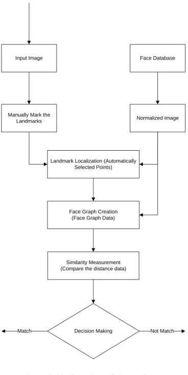
EBGM algorithm consists of five important stages: Normalization, Landmark Localization, Face Graph Creation, Similarity Measurement and Decision Making, shown in Figure 2.12.

(33)

24

Input Image Face Database

Manually Mark the

Landmarks Normalized Image

Landmark Localization (Automatically Selected Points)

Similarity Measurement (Compare the distance data)

Decision Making Face Graph Creation

(Face Graph Data)

Match Not Match

Figure 2.12 Flowchart of the EBGM

2.5 Face Recognition Approaches

2.5.1 Appearance-Based Approach

Most current face recognition techniques are only referred to the appearance-based recognition work since late 1980’s (Draper et al., 2003). The appearance based approach uses the holistic texture features and it is applied to either whole-faces or specific regions in a face image (Delac, Grgic & Grgic, 2005; Zhao, 2003). For example the algorithms such as Principal Component Analysis (PCA), Independent Component Analysis (ICA), Linear Discriminant Analysis (LDA), Support Vector Machines

(34)

25

(SVM), Neural Networks and Statistical Methods are working well for classifying frontal face in face recognition (Heisele et al., 2001; Rowley et al., 1998).

However, those algorithms are highly sensitive to translation and rotation of the target face. Therefore, before classifying the face, an alignment stage can be added to avoid this defect. The face alignment will be used to computing correspondences between two images. The correspondence determined by the prominent points in the face such as eyes and corners of the mouth is shown in Figure 1.1.

2.5.2 Module-Based Approach

There are enormous face recognition techniques referring to module-based recognition. The Module-Based approach uses geometric facial features such as mouth, eyes, nose, brows, cheeks etc) and geometric relationships between them (Brunelli & Poggio, 1993).

In fact, the idea of module-based approach is to avoid the defect of pose changed by allowing a flexible geometrical relation between the face data in the classification process such as EBGM. The Module-Based Approach includes the algorithms such as EBGM, 3D Morphable Model, 3D Face Recognition and Dynamic Link Architecture (DLA) (Moghaddam et al., 2003).

2.5.3 Advantages and Disadvantages

There are few advantages and disadvantages of using appearance-based approach and module based approach.

In appearance-based approach, the information of the images will not be destroyed because the concentration only focused on limited regions or pixel points. The appearance-based approach also has faster processing speed. However, it does not perform effectively once the target face changes the pose, in the lighting of changing environment.

In module-based approach, it is designed to recognize a target face with pose change and lighting change. Moreover, the algorithms in module-based approach are also designed to distinguish twins. However, the obvious disadvantage of using module-based approach is the difficulty of allocating the facial feature automatically. The processing speed is slow and it is not suitable for real-time face recognition purpose.

(35)

26

2.6 Evaluations and Comparisons of Algorithms

There are two types of face recognition algorithms: Procedural Algorithms and Training Algorithms. The Procedural Algorithms includes DLA, and EBGM. The Training Algorithms include PCA, LDA, ICA, SVM, and Neural Networks. The Procedural Algorithms most likely require operator involved to manually allocate the facial points. The Training Algorithms are machine learning process. The identification stage is relying on the comparison of the testing classes and the training classes.

In this research, the PCA algorithm has been selected for the experiment with the below reasons:

1) PCA is more efficient comparing to LDA, ICA and SVM. However, this is closely

related to the testing environments. There is no significant standard to distinguish which the algorithm is completely better than another.

2) PCA uses less computational time comparing to ICA and LDA when Euclidean

Distance is used.

3) PCA supports multiple input images where LDA only supports single input image

(Kim et al., 2007).

Although face recognition algorithms have been studied for a long time, there is little agreement for the performance and accuracy.

The comparison of the definition, pros and cons of the PCA algorithm and the LDA algorithm are presented in Table 2.1.

Table 2.1 Comparison of PCA and LDA

PCA LDA

Definition Principal Component Analysis

(PCA) is referred as Eigenface which is face recognition used to reduce the dimension of the face image data by means of density.

Linear Discriminant Analysis (LDA) is referred as Fisherface which is a statistical approach for classifying samples of unknown classes based on training samples with known classes. The result comparison between input image class and trained samples class will be used for decision making.

(36)

27 amount of memory required. Small face image size.

Cons It is highly sensitive to lighting,

head rotation. Because the

eigenfaces also record the lighting

information as discussed in

Section 2.3.1.

The PCA face images contain limited information.

Heavy storage.

Highly sensitive to self-shadowing, specularite (finsherface) and noise.

2.7 Moving Object Removal (MOR)

The Moving Objects Removal (MOR) is a way to remove the moving objects from the input video by using frame differencing technique. The frame differencing is a technique which checks the difference between two video frames (Prabhakar et al., 2012). The frame differencing algorithm (Jain and Nagel, 1979; Haritaoglu et al., 2000) is used to separate both static objects and dynamic objects. The static objects are considered as not moving and the dynamic object is considered as moving. Two important subjects needed to be studied in this research are moving objects detection and moving object removal.

2.7.1 Moving Object Detection (MOD)

Moving Objects Detection (MOD) in vision is a task to find the moving objects in a video frame sequence. As the movement of an object in a video frame sequence caused by pixels changing, therefore, the easiest way to extract the moving objects from a video frame sequence is to use frame difference algorithm.

The frame difference could be calculated as shown in equation (2.19). Once the objects moving in the video frames, the changes of those pixels will be presented by frames difference, is shown in Figure 2.15.

𝐷𝑖𝑓𝑓_{(𝑓1,𝑓2)} = |𝐹₍₂₎− 𝐹₍₁₎| (2.19)

The video frames shown in Figure 2.13 consist of three people, two people did not move and one person is moving pass behind the target user.

(37)

28

Figure 2.13 Sample frames of the original video footage

After applying the frame subtraction, the output video frames sequence is divided into two areas as shown in Figure 2.14. The first area is the black colour area. The black area is represented by the static objects which means there is no changes between the selected two frames and the result pixel subtraction will be 0. The second area is white colour area. An object is moving in the video frames, the result of the frame subtraction will be either greater than 0 or less than 0. In addition, the pixel changing direction also shows the possibility of the moving direction as shown in Figure 2.14.

(38)

29

2.7.2 Moving Object Removal (MOR)

In this thesis, detecting a moving object is not enough. After detection stage, we need to apply moving object removal. In other words, we have to removal the moving object and update the background. To achieve this purpose, the simple frame subtraction will be not enough. Instead, we have to compare each of the frame pixels between two frames to indicate and locate the pixel changes, the output of the MOR is shown in Figure 2.15.

(39)

30

Chapter 3 Research Methodology

The research methodology explains key research questions developed from literature review in the field of face recognition. It is a key factor to lead the success of this research. In this thesis, the research has been consistently implemented and followed. Seven steps are required to be conducted in this research. The first step is to formulate a research problem which is presented in Section 3.3, the second step is to conceptualise a research design which is described in Section 3.4.1, the third step is to construct and instrument for data collection, which is illustrated in Section 3.4.2, the forth step is to identify any limitations of the research which is given in Section 3.5, the fifth step is to predict the research output and state out research expectation in Section 3.6, the sixth step is to apply research methods and gain the experiment result in Section 4.3 and 4.4 and the seventh step is to discuss the result to analyse and evaluate whether or not the research solution can solve the research problems or issues. The accuracy of face recognition is found to be one of concerns in computer vision. As technology advances, more and more face recognition algorithms are discovered and experimented. However, there is no research undertaken with regard to moving object removal (MOR) in face recognition system. To the best of my knowledge, this is the first time face recognition in complex environments is considered with the solution of MOR.

(40)

31

3.1 Introduction

Research methodology is a way to systematically solve the key research problems deployed from literature review in the field of face recognition. The challenges and current achievements of face recognition in complex background are presented in related studies section. The accuracy of face recognition is found to be the main concern in face recognition especially in a complex environment. There are many face recognition algorithms that experimented and presented in digital image processing. There are considerable similar researches of face detection in complex background. However, there is no research with regard to apply MOR on face recognition system so as to increase face recognition precision and recall rate. To the best of my knowledge, this is the first time face recognition in complex environments taken into consideration. In this chapter, the research problems and hypothesises are discussed in details with relevance to the research gap identified from the literature review in Chapter 2. The main purpose of this chapter is to identify the research problems and explain research design, data collection, and experiment test bed.

There are five sections included in this chapter which cover the details of the research problems, hypotheses and relevant research designs. In Section 3.2, it covers the related studies of the research background. In Section 3.3, it identifies the research questions and hypotheses. In Section 3.4, a proper research design is presented and relevant data requirements are presented. In Section 3.5, the research limitations are clarified and the expected outcomes are presented in Section 3.6.

3.2 Related Work

In this section, the concept of face recognition is introduced and the previous research is presented.

Face recognition is a way to automatically identify and verify a person from a digital image or a frame of a digital video. Many image processing algorithms were proposed and experimented for face recognition. Some popular algorithms such as PCA, LDA and ICA for automatic face feature extraction and real-time face recognition are from appearance-based approach. The face recognition algorithms such as Principal Component Analysis (PCA), Linear Discriminant Analysis (LDA), 2-Dimensional Principal Component Analysis, and Independent Component Analysis (ICA) have been widely studied in the past decades. The algorithms from module-based approach such as

(41)

32

Elastic Bunch Graphic Matching (EBGM), 3-D Morphable Model and 3-D face recognition have solved the issues of the post changing in face recognition. However, the processing speed of those algorithms is one of the challenges when applied to real-time face recognition.

The researches of the face detection in complex backgrounds have achieved very remarkable results, the typical algorithms with long impact includes adaptive boosting (Adaboost) proposed by Freund and Schapire in 1996 (Chen et al., 2010). It is a machine learning algorithm which provides an effective learning algorithm and strong bounds on generalization performance in object detection (Viola & Jones, 2001; Manjunath et al., 1992; Wang & Yuan, 2001; Georghiades et al., 2001; Huynh-Thu et al., 2002; Pai et al., 2006; Li & Wang, 2013). Some researchers have experimented the face detection in complex background such as Lee et al., 1996 used motion and color information to locate human face automatically (Lee et al., 1996), Lin, 2007 and Kovac et al., 2003 presented the face detection using skin color clustering such as YCbCr (Lin, 2007; Kovac et al., 2003).

In general, face recognition in complex backgrounds is studied in four steps: 1) Locate face based on the feature and template (such as eyes, nose and mouth); 2) Use curve fitting to segment the face in image (face shape based); 3) Frontal face normalization; 4) Recognize faces with eigenface method. However, the accuracy of face recognition still yet takes into consideration since the faces to be detected and recognized are not suitable for recognition (Wu & Yang, 2004).

Yuan et al. proposed a method to detect frontal face in a complex environment by using image segmentation and face detection. The face detection consists of Valley-like detector and face verification with positive-negative attractor (Yuan et al., 2002). The Valley-like detector distinguishes the differences between surrounding pixels and core pixels in a mosaic image. The positive-negative is used to identify the positive attractor such as eyes and mouth, the negative attractor such as the surround pixel. However, all of the previous studies focused on the face detection and recognition without filtering the related face or not related face.

(42)

33

3.3 The Research Questions and Hypothesis

As mentioned in Chapter 1, the purpose of this research thesis is to propose a scheme of human face recognition in complex environments and the main objective of this thesis is to evaluate the current issues and prove the proposed scheme can increase the face recognition accuracy in complex environments such as office, reception, station and casino etc. In those environments, we set the camera always points in the fixed direction and the only changes are the moving objects such as the walkers and moving vehicles. According to the purpose of the research, there are three points needed to be taken in consideration. The first point is to understand face detection and face recognition. The second point is to understand how to simplify the complex environments. The third point is the measurement. How we measure the result indicates that to what extent the proposed scheme can increase the accuracy of face recognition.

Face recognition is a type of biometrics that can recognize a human face by analysing and comparing the face patterns, which is used to automatically identifying or verifying a person from a digital image or a video frame. There are many algorithms in face recognition such as Principal Component Analysis (PCA), Linear Discriminant Analysis (LDA), Independence Component Analysis (ICA) and Elastic Graph Bunch Matching (EGBM). The details of each algorithm were discussed in Chapter 2.

The precision, recall and F-measure will be calculated based on the experimental results. The experimentation is divided into two parts, the first one is to apply the face recognition without moving object removal and the second one is to apply the face recognition with moving object removal. In those experiment environments, precision, recall and F-measure comparison will be used to evaluate the proposed solution.

This research thesis attempts to identify a successful solution for the following research question:

“Whether the face recognition accuracy in complex environments can be increased by applying moving object removal technology?”

This research attempts to find the solutions for the following questions developed from the above main question:

1) What are the face recognition algorithms and which algorithm is the best one for

(43)

34

2) What is the moving object removal (MOR) and how could it help to improve the

face recognition accuracy in complex environments?

3.4 Research Design and Data Requirements

3.4.1 Research Design

The research design is explicitly same as this thesis structure presented in Figure 1.1. The main objective of this thesis is to find a new way to increase the precision of face recognition in complex environments.

In this research thesis, it consists of 5 main parts: motivation and objectives, literature review, research methodology, experiments, results, discussion and conclusion. There are two experimental methods were implemented in this research is shown in Figure 3.1. The first experiment process includes: face detection and face recognition. The second experiment process includes: moving object removal, face detection and face recognition.

The first experimental method consists of two stages. The first stage is face detection. In this thesis, the OpenCV cascade classification was implemented for face detection. The related study of face detection using cascade classifier was presented in Section 2.1. The second stage is face recognition and the PCA algorithm was used in face recognition as suggested in Section 2.6.

The second experimental method consists of three stages. The first stage is MOR. In this stage, the frame difference was conducted and the detail study was presented in Section 2.7 Chapter 2. The second stage is face detection. In this thesis, the OpenCV cascade classification was implemented for face detection. The related study of face detection using cascade classifier was presented in Section 2.1. The third stage is face recognition and the PCA algorithm was used in face recognition system as suggested in Section 2.6.

(44)

35

(a) (b)

Figure 3.1 Two research workflows

As shown in Figure 3.1, the face recognition in complex environments with and without MOR are the two critical experiments. There are three important phases, needed to be taken in consideration which is shown in Figure 3.2. The first phase is MOR, the second phase is face detection and the last phase is face recognition.

(45)

36

Figure 3.2 Three main phases included in the proposed scheme

Phase 1: Moving Object Removal

In MOR phase, we have to perform two tasks, the first one is the moving object detection and the second one is the moving object removal. The detailed study was presented in Section 2.7.

Moreover, the dynamic objects could also be divided into two types. The first type is represented as low speed motion object and the second type is represented as high speed motion object. As shows in Figure 3.3, the high speed motion objects are considered as background moving objects.

(46)

37

Figure 3.3 An image with high speed object and low speed object

After MOR phase, we will apply face detection in face recognition phases.

Phase 2: Face Detection

In face detection, the face detection face features must be extracted. The face features are defined as face objects such as eyes, nose, and mouth. To automatically detect those features, the OpenCV Cascade Classifiers has been used in this thesis. The OpenCV Cascade Classifiers was proposed by Paul Viola and Michael Jones in 2001 (Viola & Jones, 2001). It is also known as Viola-Jones object detection framework. The OpenCV Cascade Classifier is not only able to detect whole face and its features, but also human body shown in table 3.1. The second stage is decision making, it detects whether those detected features can group as a human face or not. The frontal face classifier was used to evaluate whether a frontal face detected or not. As a result, even if some features were detected, it is not considered as a face.

Table 3.1 OpenCV cascade classifiers

Face Features Harr Feature Based Cascade Classifier

Size

Description

Eyes haarcascade_eye.xml 20×20 Frontal eye detector.

Eyes with

glasses

haarcascade_eye_tree_e yeglasses.xml

20×20 Tree-based frontal eye detector with better handling of eyeglasses.

Frontal face haarcascade_frontalface

_alt.xml

20×20 Stump-based gentle adaboost frontal face detector.

(47)

38

_alt_tree.xml

20×20 Stump-based gentle adaboost frontal face detector. This detector uses tree of stage classifiers instead of a cascade.

_alt2.xml

20×20 Tree-based gentle adaboost frontal face detector.

_default.xml

24×24 Stump-based discrete adaboost frontal face detector.

Full Body haarcascade_fullbody.x

ml

"Haar"-based Detectors For Pedestrian Detection.

Left eye haarcascade_lefteye_2sp

lits.xml

20×20 Tree-based left eye detector. The detector is trained by 6665 positive samples from FERET, VALID and BioID face databases.

Lower body haarcascade_lowerbody.

xml

19×23 Lowerbody detector.

Eye pair haarcascade_mcs_eyepa

ir_big.xml

45×11 Eye pair detector computed with 7000 positive samples.

Eye pair haarcascade_mcs_eyepa

ir_small.xml

22×5 Eye pair detector computed

with 7000 positive samples.

Left ear haarcascade_mcs_leftea

r.xml

12×20 Left ear (in the image) detector computed with 5000 positive and 15000 negative samples.

Left eye haarcascade_mcs_leftey

e.xml

18×12 Left eye (in the image) detector computed with 7000 positive samples.

Mouth haarcascade_mcs_mout

h.xml

25×15 Mouth detector computed with 7000 positive samples.

Nose haarcascade_mcs_nose.

xml

18×15 Nose detector computed with 7000 positive samples.

(48)

39

Right ear haarcascade_mcs_righte

ar.xml

12×20 Right ear (in the image) detector computed with 5000 positive and 15000 negative samples.

Right eye haarcascade_mcs_righte

ye.xml

18×12 Right eye (in the image) detector computed with 7000 positive samples.

Head and

shoulders

haarcascade_mcs_upper body.xml

22×20 Head and shoulders detector.

Profile face haarcascade_profileface.

xml

20×20 Profile face detector.

Right eye haarcascade_righteye_2

splits.xml

20×20 Tree-based right eye detector. The detector is trained by 6665 positive samples from FERET, VALID and BioID face databases.

Smile haarcascade_smile.xml Smile detector.

Upper body haarcascade_upperbody.

xml

(49)

40

Phase 3: Face Recognition

In this phase, face recognition is considered in three tasks: feature extraction, projection, and comparison. In face recognition, two sets of class are required. The first class is input face images, also called training class. The second class is the face database images, called test classes.

In feature extraction, the PCA algorithm will be used to extract the most relevant information from an input image and represent that information in a lower dimension space. For instance, a 200 × 200 dimensional image could generate 40,000 eigenvectors. However, not all of those eigenvectors are related to the face features. The key function of PCA is to reduce the high dimensional to lower dimensional, the purpose is to focus on the most of the useful information from an image and remove the information not useful.

In projection, the PCA will precisely decompose the face structure into orthogonal components as known as eigenface. Each of projected face will be represented as a weighted eigenvector of the eigenfaces.

In comparison, the projected input face image is used to compare with the projected trained face images. The nearest distance between the input image feature vector and trained image feature vectors will be used to measure the matching face.

3.4.2 System Architecture

In order to understand the working flow of the proposed scheme, the flowcharts are one of the important and indispensable components.

In this thesis, we have presented three important flowcharts. The first flowchart is shown in Figure 3.4 as the overall system workflow. The second flowchart as shown in Figure 3.5 is the workflow of face detection and recognition and the third flowchart as shown in Figure 3.6 is for the moving object removal.

In Figure 3.4, the proposed scheme consists of three kinds of input, corresponding processing components and one output. Face recognition which we developed accepts three types of input such as video clips, images and frames of live camera. After the input resource is provided, we will then process the environment by removing all the moving objects and then the processed video will be sent to face detection and

(50)

41

recognition unit. The outputs of this proposed scheme also support video clip output and image output.