ISSN: 2302-9285, DOI: 10.11591/eei.v7i3.1181 377
Weather Forecasting Using Merged Long Short-term Memory
Model
Afan Galih Salman1, Yaya Heryadi2, Edi Abdurahman3, Wayan Suparta4 1,2,3
Computer Science Department, BINUS Graduate Program-Doctor of Computer Science, Bina Nusantara University, Jakarta 11480, Indonesia, Indonesia
4
Department of Electrical Engineering, Faculty of Science and Technology, Sanata Dharma University, Yogyakarta 55282, Indonesia
1
Computer Science Department, School of Computer Science, Bina Nusantara University, Jakarta 11480, Indonesia, Indonesia
Article Info ABSTRACT
Article history:
Received March 27, 2018 Revised May 29, 2018 Accepted Jun 12, 2018
Over decades, weather forecasting has attracted researchers from worldwide communities due to itssignificant effect to global human life ranging from agriculture, air trafic control to public security. Although formal study on weather forecasting has been started since 19th century, research attention to weather forecasting tasks increased significantly after weather big data are widely available. This paper proposed merged-Long Short-term Memory for forecasting ground visibility at the airpot using timeseries of predictor variable combined with another variable as moderating variable. The proposed models were tested using weather timeseries data at Hang Nadim Airport, Batam. The experiment results showedthe best average accuracy for forecasting visibility using merged Long Short-term Memory model and temperature and dew point as a moderating variable was (88.6%); whilst, using basic Long Short-term Memory without moderating variablewasonly (83.8%) respectively (increased by 4.8%).
Keywords:
Merged Long Short-term Memory
Weather forecasting
Copyright © 2018 Institute of Advanced Engineering and Science. All rights reserved. Corresponding Author:
Afan Galih Salman,
Computer Science Department, BINUS Graduate Program-Doctor of Computer Science, Bina Nusantara University, Jakarta 11480, Indonesia, Indonesia.
Email: [email protected]
1. INTRODUCTION
Over decades, weather forecasting has attracted researchers from worldwide communities due to its effect to the global human life. For example, farmers’ ability to predict weather fluctuations several months in advance will contribute to better harvest yields and profit. Among those weather variables, visibility prediction is significantly importantfor Air Traffic Control (ATC) of any airport in controlling planes’ landing and taking off. Formal study on weather forecasting has been started since 19th century, for example the study by Gregg [1], resulted in a vast number of methods available in literature. However, weather forecasting task regained significant attention after weather big data become widely available thanks to popularity of deep learning that helps researchers to explore hidden pattern in the large weather dataset.
In general, weather forecasting, which is a task to predict the conditions of the atmosphere for a given location and time, is an interesting computer vision problem with wide potential applications. Despite many models have been proposed, weather forecasting based on ground-based observation data remains a challenging task. According to studies by Baklanov et al. [2] and Maunder J. RW Katz and AH Murphy [3], the main challenge of weather forecasting is due to the fact that weather condition is the result of a complex process which is quite difficult to formulate in single mathematical model. In the limited scope, many researches have attempted to build weather forecasting models using statistical methods to predict weather using single or multiple variables as predictors.
The high popularity of machine learning and deep learning methods in the past ten years have motivated many researcher to propose such methods for weather forecasting tasks. For example: neural network or NN [4], recurrent neural networks or RNN [5], NN fuzzy wavelet model [6], [7], chaotic oscillary-based NN [8], ensemble of NN models [9] and hybrid of convolutional neural networks and Long Short-term Memory (LSTM) model [10]. Bedaiko [11] developed an approach based on using various complex networks metrics extracted from climate networks with Long short-term memory neural network to forecast ENSO phenomenon. The study by Ta Chu & Chia Ho [12] attempted to employ convolutional recurrent neural networks for weather temperature estimation using only image data.
Although many models have been proposed over the past ten years, there is no single model which predict weather variables with high accuracy. In addition, most of prominent weather forecasing models only used predictor variable(s) as input. The novelty of the proposed method for forecasting a weather variable is the used of moderating variable(s) and merged Long Short-term Memory Model (merged-LSTM), an exteded LSTM model proposed by [13], [14].
The premise of this study is that two patterns in the input timeseries might rectify the patterns and strengthen ability of machine learning algorithm to learn from the training data. In an attempt to achieve a robust model of learning and recognizing weather pattern, this research will explore several weather variables as moderating variable to forecast visibility variable. Therefore, the purposes of this research are two folds: (1) developing a merged-LSTM model to predict visibility variable using another weather variable as moderating variable and (2) analyzing and comparing the effect of moderating variable to visibility variable prediction.
2. RELATED RESEARCH
In the last decade, many significant efforts to solve weather forecasting problem using statistical modeling including machine learning techniques with successful results have been reported.
In 2015 Sitanggang developed a classifier for predicting hotspots occurrence using the spatial classification algorithm namely the spatial decision tree algorithm [15]
Salman propose Recurrent Neural Network (RNN) using heuristically optimization method for rainfall prediction based on weather dataset comprises of ENSO [5].
In 2017 Xingxian propose ConvLSTM with the Trajectory GRU (TrajGRU) model to predict the future rainfall intensity in a local region over a relatively short period of time that can actively learn the location-variant structure for recurrent connections.TrajGRU is more efficient in capturing the spatiotemporal correlations than ConvGRU [10]. Seongchan Kim propose model to predict the amount of rainfall from weather radardata, which is three-dimensional and four-channel data, using convolutional LSTM (ConvLSTM). ConvLSTM is a variant of LSTM (Long Short-Term Memory) containing a convolution operation inside the LSTM cell. Experimental results show that two-stacked ConvLSTM reduced RMSE by 23.0% compared to linear regression [16].
Isabelle Roesch propose method to a recurrent convolutional neural network that was trained and tested on 25 years of climate data to forecast meteorological attributes, such as temperature, air pressure and wind speed. The presented visualization system helped the user to quickly assess, adjust and improve the network design [17]. Aditya Grover propose a hybrid approach model that combines discriminatively trained predictive models with a deep neural network that models the joint statistics of a set of weather-related variables. The result show how the base model can be enhanced with spatial interpolation that uses learned long-range spatial dependencies [18].
In 2018 Kulkarni propose remote sensing technology opened for examining the weather forecasting. It helps to change to gather and analyse weather data and use to build the database for weather forecasting [19].
3. RESEARCH METHOD
3.1. Dataset and Data Preprocessing
Dataset for this research was obtained from Weather Underground (https://www.wunderground.com/) which collects weather data including temperature, dew point, humidity and visibility from many weather stations all over the world. The range of data for this study wasfrom year 2012 to year 2016 comprise of 40,025timeseries data.
The main data preprocessingsapplied to raw visibility timeseries data are: normalization in Equation 1, rescaling into range [0,1] in Equation 2 and smoothing using moving average (MA) with lag=9 in Equation 3. Consider weather time series data in 𝑇 time interval: 𝑋 = [𝑥1, 𝑥2, … , 𝑥𝑇]
𝑥𝑡= 𝑥𝑡−𝑥̿ 𝑠𝑥 (1) 𝑥𝑡′= 𝑥𝑡−𝑥𝑚𝑖𝑛 𝑥𝑚𝑎𝑥−𝑥𝑚𝑖𝑛 (2) 𝑥𝑡′′ = 1 9(𝑥𝑡 ′+ 𝑥 𝑡−1′ + ⋯ + 𝑥𝑡−8′ ) (3)
Where: 𝑥𝑡 is observation at t, 𝑥𝑡′is normalized data at t, and 𝑥𝑡′′ is the result of data smoothing using moving average at t. Correlation between two weather variables are measured using coefficient correlation (𝑟) that was computed using Equation 4.
𝑟 = 1 𝑇−1∑ ( 𝑥𝑡−𝑥̅ 𝑠𝑥 ) ( 𝑦𝑡−𝑦̅ 𝑠𝑦 ) 𝑇 𝑡=1 (4)
Where: −1 ≤ 𝑟 ≤ 1; 𝑠𝑥 and 𝑠𝑦 are standard deviation variable 𝑋 and 𝑌 respectively which were computed using the following formula:
𝑠𝑥= √
∑𝑇𝑡=1(𝑥𝑡−𝑥̅)2
𝑇−1 and 𝑠𝑦= √
∑𝑇𝑡=1(𝑦𝑡−𝑦̅)2
𝑇−1 (5)
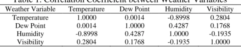
Coefficient correlation between two weather variables after being preprocessed are summarized in Table 1. In the Table 1, there is only temperature and humidity that show strong negative correlation.
Table 1. Correlation Coefficient between Weather Variables Weather Variable Temperature Dew Point Humidity Visibility
Temperature 1.0000 0.0014 -0.8998 0.2804
Dew Point 0.0014 1.0000 0.4287 0.1768
Humidity -0.8998 0.4287 1.0000 -0.1935
Visibility 0.2804 0.1768 -0.1935 1.0000
As can be seen from Table 1, temperature, dew point and humidity has low correlation with visibility so that each of these variables can become candidate for moderating variable for the proposed forecasting model. Finally, the transformed data were segmented to generate overlapping training segment (length=100/segment) and testing segment (length=2/segment) which produced 39,821 segments for both datasets. Finally, for model cross-validation purposes, the total training data was divided randomly into 27,915 (70%) training and 11,906 (30%) testing dataset.
3.2. Model Structure
Weather forecasting to be addressed in this study can be categorized as a regression problem. To solve this problem, this study proposes LSTM model which is a deep learning model proposed by [13] and improved by [14]. The model has been succesfully used in many research fields such as: large scale image classification [20], video classification [21], natural language processing [22] anomaly detection [23], [24]. In this study, LSTM was used as a foundation for weather forecasting model because of several reasons mainly:(1) the model ability to solve long lag relationship in timeseries data (2) the model ability to address vanisihing gradient problem that commonly happen in training deep structure neural networks [13].
Given a weather variable as the predictor variable and another weather variable as moderating variable, the general structure of merged-LSTM model can be illustrated in Figure 1.
Figure 1. The structure of merged-LSTM model
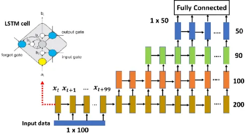
The detail structure of each LSTM model are shown in Figure 2. As can be seen from Figure 2, the proposed model is a stacked LSTM with subsequent layers having 200, 100, 90, and 50 nodes of hidden layers. The last part of the model is a fully connected neural network with 1 output nodes.
Figure 2. Structure of LSTM model
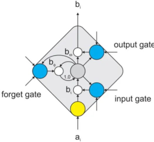
LSTM’s memory cell is a basic unit of LSTM model whose structure can be illustrated using Figure 3. As described by [13], [14], each memory cell contains input gate that learns to protect the constant error flow within the memory cell from irrelevant inputs. Output gate unit learns to protect other units from irrelevant memory contents stored in the memory cell. Forget gate unit learns to control the extent to which a value remains in the memory cell.
Figure 3. Structure of LSTM cell (Source: Sundermeyer, Schlüter & Ney, 2012)
Given a merged of two LSTMs (LSTM) model. The objective function of the merged-LSTM, ℒ, can be formulated as follows:
ℒ =1 𝑁∑ (𝑦𝑡− 𝑦̂𝑡) 2 𝑁 𝑡=1 (6) 𝑦̂𝑡= 𝜎(∑𝑚𝑡=1𝑤𝑡𝑥𝑡+ 𝑏) (7) 𝑥𝑡= 1 2(ℎ(𝑃𝑡) + ℎ(𝐼𝑡)) (8)
Where; 𝑥𝑡be the input signal to Fully Connected (FC) part of merged-LSTM as the average of predicted values from each LSTM, 𝑏 be bias
𝑦̂𝑡be predicted value, 𝑦𝑡be actual value, 𝑁 be the total number of training samples,
𝜎 be activation function,𝑥𝑡 input to FC,
ℎ(𝑃𝑡)be output of LSTM-1 whose input is the predictor variable,
ℎ(𝐼𝑡)be output of LSTM-2 whose input is the moderatingvariable(s).
Output from each LSTM cell (see Figure 3), ℎ𝑡, is computed using the following formula:
𝑓𝑡= 𝜎𝑔(𝑊𝑓𝑥𝑡+ 𝑈𝑓ℎ𝑡−1+ 𝑏𝑓) (9)
𝑖𝑡= 𝜎𝑔(𝑊𝑖𝑥𝑡+ 𝑈𝑖ℎ𝑡−1+ 𝑏𝑖) (10)
𝑜𝑡= 𝜎𝑔(𝑊𝑜𝑥𝑡+ 𝑈𝑜ℎ𝑡−1+ 𝑏𝑜) (11)
𝑐𝑡= 𝑓𝑡∘ 𝑐𝑡−1+ 𝑖𝑡∘ 𝜎𝑐(𝑊𝑐𝑥𝑡+ 𝑈𝑐ℎ𝑡−1+ 𝑏𝑐) (12)
ℎ𝑡= 𝑜𝑡∘ 𝜎ℎ(𝑐𝑡) (13)
Where: 𝑓𝑡 be forget gate’s activation vector; 𝑖𝑡 be input gate’s activation vector; 𝑜𝑡 be output gate’s activation vector; 𝑊𝑓, 𝑊𝑖, 𝑊𝑜,𝑈𝑓, 𝑈𝑖, 𝑈𝑜 are weight matrices to be learned during model training; 𝜎 be activation function; and ∘ be element-wise multiplication (Hadarmard product).
In this study two LSTM models were explored: (1) an LSTM model as a single model which was trained using visibility timeseries to forecast visibility and (2) a merged-LSTM model which was trained by two timeseries: visibility and moderating variable to forecast visibility.
3.3. Model Training and Cross-validation
In this study, the LSTM and merged-LSTM model were trained supervisedly using Adam algorithm to obtained model parameter prediction that optimized a predetermined objective function. In this model training process, model cross-validation used Leave-one-out technique with 70:30 proportion of training and
testing datasets. The proportions of training and testing dataset are set out purposively. Model performance was measured using accuracy and mean square error (MSE) metrics as formulated in equation (2.5).
4. RESULTS AND DISCUSSION 4.1. Dataset and Data Preprocessing
Histograms of raw data and smoothed data using 3-moving average are shown in Figure 4. From Figure 4(a), It appears that the raw data distribution is rather skewed. Despite being skewed; however, after being preprocessed, the data distribution looked a bit smoother.
(a) (b)
Figure 4. Visibility data distribution: (a)Raw data, and (b)After preprocessed
4.2. Model Training and Testing
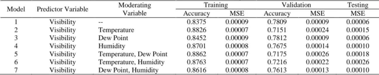
In this research, 8 models have been explored. The training performances of each model (epochs=500) to forecast visibility variable using one (two) moderating variable(s) were summarized in Table 2.
Table 2. Performance Evaluation of LSTM and merged-LSTM*to Forecast Visibility
Model Predictor Variable Moderating Variable Training Validation Testing
Accuracy MSE Accuracy MSE MSE
1 Visibility -- 0.8375 0.00009 0.7809 0.00009 0.00006
2 Visibility Temperature 0.8826 0.00007 0.7151 0.00024 0.00015
3 Visibility Dew Point 0.8452 0.00009 0.7812 0.00009 0.00006
4 Visibility Humidity 0.8701 0.00008 0.7675 0.00014 0.00010
5 Visibility Temperature, Dew Point 0.8862 0.00007 0.7175 0.00026 0.00018
6 Visibility Temperature, Humidity 0.8763 0.00007 0.7216 0.00022 0.00026
7 Visibility Dew Point, Humidity 0.8616 0.00008 0.7613 0.00013 0.00010
Note: (*) merged-LSTM used a predictor variable and one (two) moderating variables as inputs; Whilst, LSTM used only predictor variable as input. MSE: mean square error.
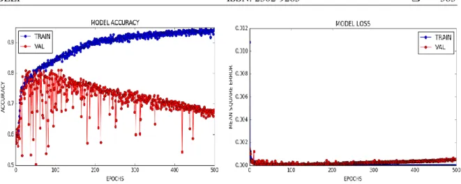
As can be seen from Table 2, for predicting visibility, the merged-LSTM with two input time series (temperature as predicted variable and dew point as moderating variable) tends to achieve higher average training accuracy than LSTM with only visibility as the input time series. The average accuracy of the former model was 88.6%; whilst, the later model only achieved 83.8% (increased by4.8%).
Figure 5. Training accuracy and loss of model merged-LSTM with temperature and dew point as moderating variable
Interestingly, although both temperature and dew point had low correlation with visibility, but these variable strengthen visibility prediction accuracy of the merged-LSTM model.Prediction result of the best model in compare with the test (actual) timeseriesis shown in Figure 6. As can be seen from Figure 6, deviation between predicted and actual test data is not so wide.
Figure 6. Comparison between predicted visibility and actual test visibility dataset using trained merged-LSTM
Figure 7. Comparison between predicted visibility for 96 future points and actual test visibility dataset using the trained merged-LSTM
With this experiment show that LSTM model is able to explain or formulate relationship among the predicted and intermediate variable. The addition of intermediate variables able to increase accuration of weather prediction. In this experiment to predict visibility with addition intermediate variables such as: temperature and combinationof temperature and dewpoint produce the best accuration and the lowest MSE compare with the prediction visibility without addition intermediate variables.
The most important findings of these research are modify of input weather data that has influence each other to find the combination weather data input that can optimize forecasting accuracy in time series data model, the combination of input weather data model which can be used for weather forecasting in Airport area and research artifacts (scripts and dataset) will be made available for other researchers in the same domain.
5. CONCLUSION
Weather forecasting task has gained wide attention from many research communities due to its significant effect to global human life. Many efforts to build weather forecasting models have been proposed resulted in a vast number of publications available in literature. However, the nature of weather is so complex that impossible to be formulated in a single mathematical model.
Despite many models have been proposed for weather prediction, most of these models used the same input and output variables. The result of this study, which exploited LSTM model variant, showed that moderating variables can improve prediction capability of the model. Based on the experiment results, the proposed merged-LSTM model improved accuracy of basic LSTM in predicting visibility by 4.8% higher. That results showed that our approach works well in predicting visibility. Based on this results, the future steps of this research is to extend this approach for forecasting various weather variables using multidimensional timeseries.
REFERENCES
[1] Gregg, Willis Ray, "Progress in weather forecasting", Electrical Engineering, 57, no. 10, pp. 405-412. 1938 [2] Baklanov. Integrated Modeling for Forecasting Weather and Air Quality: A Call for Fully Coupled Approaches.
Atmospheric Environment. Elsevier. 2011
[3] Maunder J., R.W. Katz and A.H. Murphy, economic value of weather and climate forecasts. Climatic Change, 45(3-4), pp. 601-606, 2000.
[4] Normakristagaluh. Artificial Neural Network for Rainfall Forecasting in Statistical Downscaling. Bogor. Thesis. Institut Pertanian Bogor. 2004.
[5] Afan Galih Salman, Bayu Kanigoro, Yaya Heryadi. Weather Forecasting Using Deep Learning Techiniques. ICACSIS UI Proceeding IEEE. 2015.
[6] Afshin. Long Term Rainfall Forecasting by Integrated Artificial Neural Network-Fuzzy Logic-Wavelet Model in Karoon Basin, Scientific Research and Essay 2011: vol 6(6), pp. 1200-1208.
[7] Belayneh, A. Standard Precipitation Index Drought Forecasting Using Neural Networks,Wavelet Neural Networks and Support Vector Regression. Hindawi Publishing Corporation Applied Computational Intelligence and Soft Computing Volume. 2012. .Article ID 794061, 13 pages doi:10.1155/2012/794061.
[8] Kwong, K. M, Liu, J. N. K., Chan, P. W., and Lee, R. Using LIDAR Doppler Velocity Data and Chaotic Oscillatory-Based Neural Network for The Forecast of Meso-Scale Wind Field. In Evolutionary Computation. IEEE World Congress on Computational Intelligence. 2008: pp. 2012-2019.
[9] Maqsood, I, M. R. Khan, and A. Abraham. An Ensemble of Neural Networks for Weather Forecasting. Neural Computing & Applications 13.2 .2004. 112-122.
[10] Xingjian Shi, Zhourong Chen, Hao Wang, Dit-Yan Yeung. Convolutional LSTM Network: A Machine Learning Approach for Precipitation Nowcasting, Part of: Advances in Neural Information Processing Systems 28 (NIPS) 2015.
[11] Clifford Broni-Bedaiko, Ferdinand Apietu Katsriku, Tatsuo Unemi, Norihiko Shinomiya, Jamal-Deen Abdulai and Masayasu Atsumi. El Niño-Southern Oscillation Forecasting Using Complex Networks Analysis of LSTM Networks, The Twenty-Third International Symposium on Artificial Life and Robotics 2018 (AROB 23rd 2018). [12] Wei-Ta Chu and Kai-Chia Ho. Visual Weather Temperature Prediction, arXiv:1801.08267v1 [Cs.CV]. 25 Jan
2018.
[13] Hochreiter, S. and J. Schmidhuber. Long Short Term Memory, Neural Computation. MIT 1997.
[14] Felix A. Gers, Jürgen Schmidhuber; Fred Cummins. Learning to Forget: Continual Prediction with LSTM". Neural Computation. 12 (10) 2000: 2451–2471.
[15] Imas Sukaesih Sitanggang, RazaliYaakob, Norwati Mustapha, Ainuddin A. N.A Decision Tree Based on Spatial Relationships forPredicting Hotspots in Peatlands. TELKOMNIKA, Vol. 12, No. 2, pp. 511~518, June 2014. [16] Seongchan Kim, Seungkyun Hong, MinsuJoh, Sa-kwang Song, Deep Rain.ConvLSTM Network for Precipitation
[17] Isabelle Roesch and Tobias Günther, Visualization of Neural Network Predictions for Weather Forecasting, Eurographics Proceedings.TheEurographics Association, 2017.
[18] Aditya Grover, Ashish Kapoor, Eric Horvitz, A Deep Hybrid Model for Weather Forecasting, KDD '15 Proceedings of the 21th ACM SIGKDD International Conference on Knowledge Discovery and Data Mining, KDD '15 Proceedings of the 21th ACM SIGKDD International Conference on Knowledge Discovery and Data Mining Pages 379-386 , Sydney, NSW, Australia — August 10 - 13, 2015
[19] Atul Kulkarni, Debajyoti Mukhopadhyay. Internet of Things Based Weather Forecast Monitoring System. Indonesian Journal of Electrical Engineering and Computer ScienceVol. 9, No. 3, pp. 555~557, ISSN: 2502-4752, DOI: 10.11591/ijeecs.v9.i3.pp555-557, March 2018
[20] Real, E., Moore, S., Selle, A., Saxena, S., Suematsu, Y. L., Le, Q., & Kurakin, A. Large-Scale Evolution of Image Classifiers. ArXiv preprint arXiv: 1703.01041.2017.
[21] Yoo, J. H. Large-Scale Video Classification Guided by Batch Normalized LSTM Translator. ArXiv preprint arXiv: 1707.04045.2017.
[22] Elkaref, M., & Bohnet, B. A Simple LSTM model for Transition-based Dependency Parsing. ArXiv preprint arXiv: 1708.08959.2017.
[23] Luo, W., Liu, W., & Gao, S. Remembering History with Convolutional LSTM for Anomaly Detection. In Multimedia and Expo (ICME), 2017 IEEE International Conference 2017:pp. 439-444.
[24] Lee, T. J., Gottschlich, J., Tatbul, N., Metcalf, E., &Zdonik, S. Greenhouse: A Zero-Positive Machine Learning System for Time-Series Anomaly Detection.arXiv preprint arXiv: 1801.03168.2018.