Learning with Privileged Information using Multimodal Data

(1)

Learning with Privileged Information using

Multimodal Data

Nuno Cruz Garcia

DITEN, Universit`

a di Genova

PAVIS, Istituto Italiano di Tecnologia

PhD in Science and Technology for Electronic

and Telecommunication Engineering

Curriculum: Computational Vision,

Automatic Recognition and Learning

Supervisor:

Vittorio Murino

Co-Supervisor:

Pietro Morerio

In partial fulfillment of the requirements for the degree of

Doctor of Philosophy

(2)

(3)

(4)

Acknowledgements

I had the pleasure to share these three years of PhD with a lot of kind, brilliant, and inspiring people.

The first words of deep gratitude is to my supervisor, Vittorio Murino, for the opportunity to learn from him, the guidance, the inspiration, and the mentorship. To my co-supervisor Pietro Morerio, for all the brilliant insights on deep learning, all the good ideas and experiments that make some of my favorite parts in this document. They con-stitute a research role model that I hope I can be one day to my students.

To Sarah, Vitaly, Stan, and IVC friends, for the amazing six months I spent at Boston University. The positivity, kindness, wisdom, and scientific rigor I learned in all the meetings, lunches, walks, and con-versations are lessons that go beyond research.

I’m fortunate to have crossed paths with many people that made my stay in Genova a beautiful experience. PAVIS, VGM, IIT, and Unige are incredible places to be as a young researcher. I’m grateful to Alessio del Bue, Prof. Mario Marchese, and all staff for the helpful, cooperative and lively environment. Thank you to all the friends from IIT football team, to the Portuguese friends, and to those with whom I shared fraternal evenings.

(5)

I am most grateful to my family. They are the most inspiring exam-ples I have. They teached me to follow by dreams by example, when they decided to continue to study late in life, during hard times. They teached me to be curious, to have fun, to stay focused, and to like sci-ence. To my favorite person in the world, Patr´ıcia, for the unique care, understanding and closeness. To Vanessa, for all the love, patience, and support.

(6)

”If you can think - and not make thoughts your aim” Para a minha fam´ılia.

(7)

Abstract

Computer vision is the science related to teaching machines to see and understand digital images or videos. During the last decade, computer vision has seen tremendous progress on perception tasks such as ob-ject detection, semantic segmentation, and video action recognition, which lead to the development and improvements of important indus-try applications such as self-driving cars and medical image analysis. These advances are mainly due to fast computation offered by GPUs, the development of high capacity models such as deep neural net-works, and the availability of large datasets, often composed by a variety of modalities. In this thesis we explore how multimodal data can be used to train deep convolutional neural networks.

Humans perceive the world through multiple senses, and reason over the multimodal space of stimuli to act and understand the environ-ment. One way to improve the perception capabilities of deep learning methods is to use different modalities as input, as it offers different and complementary information about the scene. Recent multimodal datasets for computer vision tasks include modalities such as depth maps, infrared, skeleton coordinates, and others, besides the tradi-tional RGB.

This thesis investigates deep learning systems that learn from multiple visual modalities. In particular, we are interested in a very practical

(8)

scenario in which an input modality is missing at test time. The question we address is the following: how can we take advantage of multimodal datasets for training our model, knowing that, at test time, a modality might be missing or too noisy? The case of hav-ing access to more information at trainhav-ing time than at test time is referred to as learning using privileged information.

In this work, we develop methods to address this challenge, with spe-cial focus on the tasks of action and object recognition, and on the modalities of depth, optical flow, and RGB, that we use for inference at test time. This thesis advances the art of multimodal learning in three different ways. First, we develop a deep learning method for video classification that is trained on RGB and depth data, and is able to hallucinate depth features and predictions at test time. Second, we build on this method and propose a more generic mechanism based on adversarial learning to learn to mimic the predictions originated by the depth modality, and is able to automatically switch from true depth features to generated depth features in case of a noisy sensor. Third, we develop a method that learns a single network trained on RGB data, that is enriched with additional supervision information from other modalities such as depth and optical flow at training time, and that outperforms an ensemble of networks trained independently on these modalities.

(9)

List of Figures

1.1 What is the best way of using all data available at training time, considering a missing (or noisy) modality at test time? . . . 2

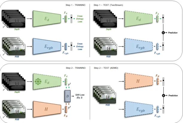
3.1 Training procedure described in section3.2.3(see also text therein). The 1st _{step represents the segregate training of the appearance}

and depth stream networks. The 2nd step illustrates the two-stream joint training. The 3rd _{step refers to the hallucination}

learning step using the soft labels with temperature si (eq. 3.6)

and the novel distillation loss L (eq. 3.7), where the weights of the depth stream network are frozen. The 4th _{step refers to a}

fine-tuning step, and exemplifies also the testing setup, in which RGB data is the only input to the model. . . 18

3.2 Detail of the ResNet residual unit, showing the multiplicative con-nections and temporal convolutions [1]. In our architecture, the signal injection occurs before the 2nd residual unit of each of the four ResNet blocks. . . 20

3.3 Example of RGB and depth frames from the NTU RGB+D Dataset.

(13)

LIST OF FIGURES

3.4 The plot shows the hallucination loss Lhall of Eq. 3.3: the gray

and blue curves refers to the model where no multiplicative con-nections are used to learn the hallucination stream (row #14 of Table 3.2). We started the experiment with learning rate set to 0.001, and continued after a while with learning rate set to 0.0001. The red curve shows instead Lhall after plugging the inter-stream

connections (row #13 of Table 3.2). . . 31

4.1 Architecture and training steps (solid lines - module is trained; dashed lines - module is frozen ). Step 1: Separate pretraining of RGB and Depth networks (Resnet-50 backbone with temporal convolutions). The bottleneck described in section 4.2.2 is high-lighted as a separate component. At test time the raw predictions (logits) of the two separate streams are simply averaged. The com-plementary information carried by the two streams bring a signif-icant boost in the recognition performance. Step 2: The depth stream is frozen. The hallucination stream H is initialized with the depth stream’s weights and adversarially trained against a dis-criminator. The discriminator is fed with the concatenation of the bottleneck feature vector and the temporal frame ordering label

yt_{, as detailed in Section}_4.2.1_{. The discriminator also features an}

additional classification task, i.e. not only it is trained to discrim-inate between hallucdiscrim-inated and depth features, but also to assign samples to the correct class (Eq. 4.2). The hallucination stream thus learns monocular depth features from the depth stream while maintaining discriminative power. At test time, predictions from the RGB and the hallucination streams are fused. . . 42

(14)

LIST OF FIGURES

4.2 Detail of the ResNet residual unit with temporal convolutions (blue block). . . 47

4.3 Architectures for the discriminators used for the two different tasks. Left: D1 for object recognition. Right: D2 for action recognition. 48

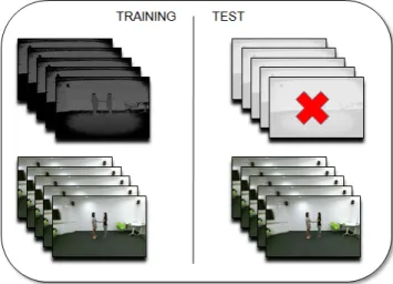
4.4 Examples of RGB and depth frames from the NYUD (RGB-D) dataset. . . 50

4.5 Discriminator confidence at predicting ’fake’ label as a function of noise in the depth frames. The more corrupted the frame, the more confident D, and the lower the accuracy of the Two-stream model (NYUD dataset). . . 60

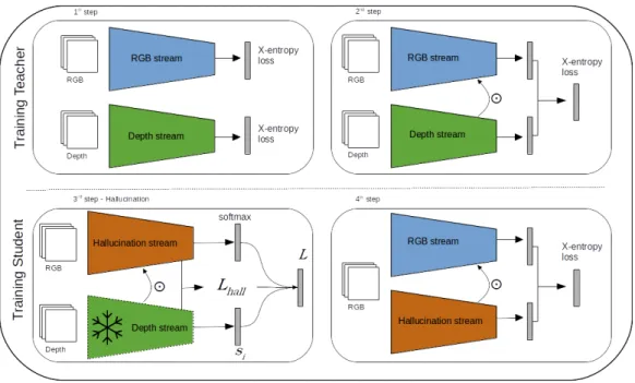
5.1 Distillation Multiple Choice Learning (DMCL) allows mul-tiple modalities to cooperate and strengthen one another. For each training sample, the modality specialistmthat achieves the lowest loss ` distills knowledge to strengthen other modality specialists. At test time, any subset of available modalities can be used by DMCL to make predictions. . . 66

5.2 Distillation Multiple Choice Learning (DMCL) In the For-ward Pass, we calculate the classification cross-entropy losses` for each modality and identify the teacher network - in this case, the Depth network. In the Backward Pass, we compute the soft targets of the teacher,SD, and use them as an extra supervision signal for

the student networks. The loss for the student networks`GD _refers

to the Generalized Distillation loss, defined on Eq. 5.3. The loss for the teacher network D uses the normal logits, i.e. soft targets with temperature T = 1. At test time, we are able to cope with missing modalities. The final prediction is obtained by averaging the predictions of the available modalities. . . 68

(15)

LIST OF FIGURES

5.3 The cross-entropy loss of three networks independently trained for action recognition on the UWA3DII dataset, using RGB (blue), depth (green), and optical flow (orange). These plots are averaged over three runs. We observe that for the first 10K steps, the train-ing loss of the optical flow network is consistently lower, result-ing in a winner-takes-all behavior in traditional MCL algorithms. However, in DMCL, the winner network also teaches the loser net-works, strengthening the other modality networks and avoiding this behavior. . . 80

(16)

List of Tables

3.1 Classification accuracies and comparisons with the state of the art. Performances referred to the several steps of our approach (ours) are highlighted in bold. ×refers to comparisons with unsupervised learning methods. 4 refers to supervised methods: here train and test modalities coincide. refers to privileged information methods: here training exploits RGB+D data, while test relies on RGB data only. . . 27

3.2 Ablation study. A full set of experiments is provided for cross-subject evaluation protocol, and for the cross-view protocol, only the most important results are reported. . . 29

3.3 Accuracy of the model tested with clean RGB and noisy depth data. Accuracy of the proposed hallucination model, i.e. with no depth at test time, is 77.21%. . . 33

3.4 Inverting the cross-stream connection study. The last section of the table refers to results where the direction of the cross-stream connection has been inverted. The other results are also reported in the paper, as they refer to the model proposed. . . 35

4.1 Ablation Study - Bottleneck size. Hallucination network under-performing with Fx ∈R2048. . . 51

(17)

LIST OF TABLES

4.2 Ablation Study - Investigating different bottleneck implementa-tions. The Table reports Hallucination network performances on NTU-mini. . . 52

4.3 Ablation Study - Investigating different inputs and tasks for the discriminator. The Table reports Hallucination network perfor-mances (NTU-mini). . . 53

4.4 Classification accuracies and comparisons with the state of the art for video action recognition. Performances referred to the several steps of our approach (ours) are highlighted in bold. × refers to comparisons with unsupervised learning methods. 4refers to supervised methods: here train and test modalities coincide. refers to privileged informa-tion methods: here training exploits RGB+D data, while test relies on RGB data only. The 4th column refers to cross-subject and the 5th to the cross-view evaluation protocols on the NTU dataset. The results reported on the other two datasets are for the cross-view protocol. . . 56

4.5 Object Recognition . . . 57

4.6 Accuracy values for the two-stream model trained on RGB and depth, and tested with RGB and noisy depth data. . . 61

5.1 Comparing MCL methods. We compare the performance of SMCL and CMCL with our proposed DMCL on the NWUCLA, UWA3DII, and NTU120 datasets. We also compare against independently trained modality networks. For each method we present the ac-curacy of the RGB modality network, the sum of all modality network predictions (P

), and the oracle accuracy (Φ). For each row, corresponding to one dataset, we highlight in bold the best result using RGB only at test time. Using our DMCL methods results in better RGB networks for three out of four datasets. . . 77

(18)

LIST OF TABLES

5.2 Selecting the right teacher network is important. We present the action recognition classification accuracy on the NWUCLA and UWA3DII datasets for three scenarios, where: modality networks are trained independently; a random teacher is assigned for ev-ery sample to guide the other modality networks; and DMCL, where the best-performing teacher (lowest loss) is selected to guide other modality networks. For each column, corresponding to a test modality, we highlight in bold the best result across the three sce-narios. . . 77

5.3 Accuracy of a KNN classifier with varying k on the NWUCLA dataset. Classified features are computed using randomly initial-ized networks for each modality. Although all features are ran-domly generated, optical flow random features tend to achieve a significantly higher accuracy. This helps to explain why optical flow networks learn faster than other modalities. . . 79

(19)

LIST OF TABLES

5.4 Accuracy for UWA3DII and NWUCLA dataset. The first part of the table refers to methods that use unsupervised feature learn-ing (*) or that use the same number of modalities for trainlearn-ing and testing. The second part of the table refers to methods that use more modalities for training than for testing. Methods that use RGB+ _{at test time use an additional network that mimics the} missing modality. For each column, corresponding to one dataset, we highlight in colored bold the best result and in normal col-ored font the second best between our method and the baselines. Each color corresponds to a different test modality. To conduct a fair comparison with baseline methods, this table presents results for the most common view setting for UWA3DII and NWUCLA. Other view settings follow the same trend and results are presented in the supplementary material. . . 83

5.5 Evaluation on NTU datasets. The test sets for NTU120mini _and

NTU120 are the same. For each column, corresponding to one dataset, we highlight in bold the best result and in normal colored font the second best between our method and the baselines. Each color corresponds to a different test modality. The approximated values are inferred from a plot in [2]. We note that the effect of the distillation method is more visible on the smaller scale versions NTU60 and NTU120mini _{of the dataset. . . .} ₈₄

(20)

Chapter 1

Introduction

1.1

Objective, Motivation, and Challenges

Depth perception is the ability to reason about space in the 3D world, critical for the survival of many hunting predators and an important skill for humans to understand and interact with the surrounding environment. It develops very early in humans when babies start to crawl [3], and emerges from a variety of mechanisms that jointly contribute to the sense of relative and absolute position of objects, called depth cues. Besides binocular cues, e.g. stereovision, humans use monocular cues that relate to a priori visual assumptions derived from 2D single images through shadows, perspective, texture gradient, and other signals

-e.g. the assumption that objects look blurrier the further they are, or that if an object occludes another it must be closer, etc. [4]. As matter of fact, although humans underestimate object distance in a monocular vision setup [5], we are still able to perform most of our vision-related tasks with good efficiency even with one eye covered.

Similarly, depth perception is often of paramount importance for many com-puter vision tasks related to robotics, autonomous driving, scene understanding,

(21)

1.1 Objective, Motivation, and Challenges

Figure 1.1: What is the best way of using all data available at training time, considering a missing (or noisy) modality at test time?

to name a few. The emergence of cheap depth sensors and the need for big data led to big multimodal datasets containing RGB, depth, infrared, and skeleton sequences [6], which in turn stimulated multimodal deep learning approaches. Traditional computer vision tasks like action recognition, object detection, or in-stance segmentation have been shown to benefit performance gains if the model considers other modalities, namely depth, instead of RGB only [7; 8; 9; 10].

However, it is reasonable to expect that depth data is not going to be always available when a model is deployed in real scenarios, either due to the impossibility to collect depth data with enough quality, e.g. due to far-distance or reflectance issues, or to install depth sensors everywhere, sensor or communications failure, or other unpredictable events.

Considering this limitation, we would like to answer the following question (depicted in Fig. 1.1): what is the best way of using all data available at training time, in order to learn robust representations, knowing that there are missing (or noisy) modalities at test time? In other words, is there any added value in training a model by exploiting multimodal data, even if only one modality is

(22)

1.1 Objective, Motivation, and Challenges

available at test time?

Unsurprisingly, the simplest and most commonly adopted solution consists in training the model using only the modality in which it will be tested. Neverthe-less, a more interesting alternative is to exploit the potential of the available data and train the model using all modalities, being however aware of the fact that not all of them will be accessible at test time. This learning paradigm,i.e., when the model is trained using extra information, is generally known as learning with privileged information [11] or learning with side information [12].

This work investigates multimodal learning with the goal to develop computer vision models that leverage the complementarity offered by diverse modalities at training time, while being robust to missing modalities at test time. We are mainly interested in developing methods that are flexible regarding the input modalities and training or evaluation tasks. The idea of learning from multimodal data while being aware that modalities may be missing at test time is central for perception in general, and in particular for the next-generation of computer vision applications e.g. concerning robotics.

The ability to reason how different data modalities relate to each other is linked to the practical low-level task of predicting one modality from the other. A classical example is depth estimation from RGB images. This task can also be defined in the feature space, rather than the input space. In this thesis, we approach this problem from a high-level perspective,i.e. we are interested in esti-mating high-level features and predictions that correspond to the depth network, instead of the actual depth map of the scene. One of the main challenges of multimodal learning is to develop a method that efficiently leverages the differ-ent advantages that diverse modalities offer. We address this problem from the more challenging perspective of being able to account for a missing modality for inference. We develop deep learning methods that learn using RGB, Depth, and

(23)

1.2 Contributions and Outline

Optical Flow data. We extensively evaluate our methods on the task of video action recognition, and also provide results on the task of object recognition. The next section discusses the main contributions of this thesis.

1.2

Contributions and Outline

This thesis will describe several models for multimodal learning using privileged information.

Chapter 2 describes the related work and places our work at the intersection of three topics, namely Generalized Distillation, Adversarial Learning, and Mul-timodal Deep Learning. Specific works that are closer to the methods presented in the following chapters are discussed within the corresponding chapter.

Chapter3introduces a model that learns from RGB and depth, and uses RGB only at test time for video action classification. This is accomplished by means of an additional network that learns to mimic the missing modality features and predictions, called hallucination network, using the modality that is available as input. This chapter is mainly based on the publication:

• [13] N. C. Garcia, P. Morerio, and V. Murino, ”Modality distillation with multiple stream networks for action recognition”, in The European Confer-ence on Computer Vision (ECCV), September 2018.

Chapter 4 extends the previous work to the task of object recognition, and presents a novel method to learn the hallucination network. We develop an ad-versarial learning strategy to align the features and predictions across modalities. We also evaluate this method using noisy data, and present a mechanism to au-tomatically switch to hallucinated features and predictions in case the input data is too noisy. This chapter is based on the publication:

(24)

• [14] - N. C. Garcia, P. Morerio, and V. Murino, ”Learning with privileged information via adversarial discriminative modality distillation”, Transac-tions on Pattern Analysis and Machine Intelligence (TPAMI), 2019. Chapter 5 investigates how multimodal data can be used in a cooperative learning setting. We present an algorithm to learn an ensemble of multimodal net-works simultaneously, that leverage the strengths of each corresponding modality to the benefit of the ensemble and themselves. This algorithm is robust to missing modalities, hence also related to the privileged information learning framework. We evaluate this method using RGB, Depth, and Optical Flow data for the task of video action recognition. This work refers to a paper under revision.

• [15] - N. C. Garcia, S. A. Bargal, V. Ablavsky, P. Morerio, V. Murino, and S. Sclaroff, ”DMCL: Distillation Multiple Choice Learning”,under revision, 2019.

Chapter6discusses future directions and applications of multimodal learning with privileged information, and in particular of techniques developed in this thesis.

1.2.1

List of Publications

To summarize the publications described in this thesis are:

• [13] N. C. Garcia, P. Morerio, and V. Murino, ”Modality distillation with multiple stream networks for action recognition”, in The European Confer-ence on Computer Vision (ECCV), September 2018.

• [16] N. C. Garcia, P. Morerio, and V. Murino, ”Chapter 12 - cross-modal learning by hallucinating missing modalities in rgb-d vision,” in Multimodal Scene Understanding (M. Y. Yang, B. Rosenhahn, and V. Murino, eds.), pp. 383 – 401, Academic Press, 2019

(25)

• [14] - N. C. Garcia, P. Morerio, and V. Murino, ”Learning with privileged information via adversarial discriminative modality distillation”, Transac-tions on Pattern Analysis and Machine Intelligence (TPAMI), 2019.

• [15] - N. C. Garcia, S. A. Bargal, V. Ablavsky, P. Morerio, V. Murino, and S. Sclaroff, ”DMCL: Distillation Multiple Choice Learning”,under revision, 2019.

(26)

Chapter 2

Related Work

The book of reference by Goodfellowet al. [17] gives a detailed perspective on the field of Deep Learning. In this chapter, we review mainly deep learning methods that are closer to our work, namely related to the topics of Knowledge Distillation, Adversarial Learning, and Multimodal Deep Learning.

2.1

Generalized Distillation

The Generalized Distillation framework, proposed in [18], gives a unifying per-spective on two distinct theories related to the concept of machines-teaching-machines: Privileged Information [11] and Knowledge Distillation [19][20]. The former, also known as Learning Using Privileged Information (LUPI), introduces to the learning process the concept of a ”teacher” model that provides additional information to a ”student” model, in addition to the label supervision. The in-tuition is that the teacher’s additional explanations enable the student to learn a better model than if it would be trained using label supervision only. Impor-tantly, the additional information provided by the teacher is only available to the student at training time, thus the term privileged information.

(27)

2.1 Generalized Distillation

On the other hand, Knowledge Distillation (KD) proposes a training proce-dure to transfer knowledge from a previously trained large model or ensemble of models to a small model, thus distilling information from a heavier to a lighter model. This idea comes from the fact that speed and computation requirements for training and testing phases are very different.

These ideas have in common the concept of machines-teaching-machines: the model used for inference learns from a model that was previously trained in a more advantageous condition, e.g. using additional information, better quality data, or simply is an aggregate of several large models. The work presented in this thesis are both related to the privileged information theory and to knowledge distillation, and address these from a multimodal perspective.

We are interested in exploring additional modalities only available at training time, such as depth and optical flow, which are considered to be privileged infor-mation in our approaches. The knowledge distillation framework is at the core of our methods as the mechanism to distill the knowledge offered by models that use the additional modalities.

The idea of using privileged information was explored in many applications. Luo et. al. [21] proposed an interesting model that is first trained on several modalities (RGB, depth, and three features joints-based), but tested only in one of these. The method uses a graph-based distillation mechanism to distill infor-mation between all modalities at training time. The training process is split in different stages, a first one of pretraining using all modalities and a large dataset, and then a second one using a subset of modalities and a smaller dataset. The test set consists of a single modality from the smaller dataset. This achieves state-of-the-art results in action recognition and action detection tasks. Learning with privileged information for action recognition has also been explored for re-current neural networks. In [22], the authors devise a method that uses skeleton

(28)

2.1 Generalized Distillation

joints as privileged information to learn a better action classifier that uses depth, even with scarce data.

The work of Hoffman et al. [12] introduced a model to hallucinate depth features from RGB input for object detection task. This approach learns the hallucination network by minimizing an Euclidean loss between the true depth features and hallucinated feature maps. In addition, the final loss function in-cludes more than ten classification and localization losses, balanced using the corresponding hyperparameters. Our work is inspired in this approach and we extend some of these ideas to other tasks, and by formulating our problem within the generalized distillation framework.

An interesting work lying at the intersection of multimodal learning and learn-ing with privileged information is ModDrop by Neverova et al. [23]. The authors propose a modality-based dropout strategy, where each input modality is entirely dropped (actually zeroed) with some probability during training. The resulting model is proved to be more resilient to missing modalities at test time.

The idea of knowledge distillation was initially applied to network compression [24], and have since then been applied in many creative ways to a variety of domains such as language tasks [25], defending from adversarial attacks [26], transfer labels across domains [27], unifying classifiers using unlabeled data [28], or using distillation without a pre-trained teacher [29] [30]. The gains provided by Knowledge Distillation are still not completely understood in the literature. With this work, we hope to provide insights on its application to multimodal data.

(29)

2.2 Adversarial Learning

2.2

Adversarial Learning

Chapter 4 is closely related to this body of work. Our method implements an adversarial strategy to generate features from the missing modality feature space, using RGB as input.

In the seminal paper of Goodfellowet al. [31], the authors propose a generative model that is trained by having two networks playing the so called minimax

game. A generator network is trained to generate images from noise vectors, and a discriminator network is trained to classify the generated images as false and images sampled from the dataset as true. As the game evolves, the generator becomes better and better at generating samples that look like the true images from the data distribution. This is usually referred to as Generative Adversarial Networks (GANs).

The concept of adversarial training was explored in many different tasks and domains other than image generation, such as disentangling semantic concepts [32], network compression [33] [34] [35], feature augmentation [36], image to image translation [37]. The training stability was improved by exploring different losses [38] and other tricks related to the implementation of GANs [39][40].

An important variant of the GAN framework are Conditional GANs (CGANs) [41], that propose to concatenate the label of desired class to be generated, to the noise vector. The CGAN model has been used in different domains, from image synthesis [42] to domain adaptation [36]. We extend the CGAN idea to achieve the goal of temporal correspondence between the generated and the target feature vectors. This is discussed in more detail in Chapter 4. Perhaps more similar to our work is the interesting paper by Roheda et al.[43], that also approaches the problem of missing modalities in the context of adversarial learning. The authors address the binary task of person detection using images, seismic, and acoustic sensors, where the latter two are absent at test time. A CGAN is conditioned

(30)

2.3 Multimodal Deep Learning

on the available images and the generator maps a vector noise to representative information from the missing modalities, with an auxiliary L2 loss. In contrast to this work, our CGAN model learns a mapping directly from the test modality to the feature space of the missing modality, with no auxiliary loss. We also focus on different tasks, namely video action recognition and object recognition.

2.3

Multimodal Deep Learning

2.3.1

RGB-D Vision

Video action recognition and object detection have a long and rich field of liter-ature, spanning from classification methods using handcrafted features, e.g. [44; 45; 46; 47; 48; 49] to modern deep learning approaches,e.g. [9; 50; 51; 52; 53; 54], using either RGB-only, representations obtained from RGB such as optical flow, depth data, or a combination of these. We point to some of the more relevant works in video action recognition and object recognition using multimodal data and also to state-of-the-art methods that consider the privileged information sce-nario or a missing modality at test time.

Multimodal Video Action Recognition

A more comprehensive review is presented in [55] [56] [57]. The two-stream model introduced by Simonyan and Zisserman [50] is a landmark on video analysis, and since then has inspired a series of variants that achieved state-of-the-art perfor-mance on diverse datasets. This architecture is composed by a RGB and an optical flow stream, which are trained separately, and then fused at the pre-diction layer. The RGB network models mainly appeareance features and the optical flow, due to being specifically designed to represent movement, models motion. In [1], the authors propose a variant of this architecture, which models

(31)

spatiotemporal features by injecting the motion stream’s signal into the residual unit of the appearance stream. They also employ 1D temporal convolutions along with 2D spatial convolutions. The combination of 2D spatial and 1D temporal convolutions has shown to learn better spatiotemporal features than 3D convo-lutions [58]. The current state of the art in video action recognition [59] uses 3D temporal convolutions and a new building block dedicated to capture long range dependencies, using RGB data only. We explore some of these architectures on Chapters 3, 4, and 5.

Some interesting works use modules specifically developed to learn motion features, which are then incorporated in models that use RGB only [60] [61] [62] [63]. Other methods learn an additional hallucination network to mimic the features of optical flow [64].

In [7], the complementary properties of RGB and depth data are explored, taking the NTU RGB+D dataset as testbed. This work designed a deep au-toencoder architecture and a structured sparsity learning machine, and showed to achieve state-of-the-art results for action recognition. Liu et al. [8] also use RGB and depth complementary information to devise a method for viewpoint invariant action recognition, extensively evaluated on the NTU RGB+D dataset. Here, dense trajectories from RGB data are first extracted, which are then en-coded in viewpoint invariant deep features, while a similar procedure is followed for the depth stream. The RGB and depth features are then used as a dictionary to predict the test label.

We mainly use three datasets for action recognition, which offer RGB and Depth data. These are the UWA3DII [65], the NWUCLA [66], and the NTU60 and NTU120 RGB+D [67] [2]. We describe these datasets in the experimental sections of the methods, along with the training and testing protocols.

(32)

Object Recognition

Over the years, object recognition based on RGB and depth have been an insight-ful task to reason on the complementarity of these two modalities, and whether depth data should be handled differently compared to RGB. An example of this is [9], in which the authors propose to encode depth images using a geocentric em-bedding that encodes height above ground and angle with gravity for each pixel in addition to the horizontal disparity, showing that it works better than using raw depth. Differently, in [54], the authors focus on carefully designing a convolu-tional neural network including a multimodal layer to fuse RGB and depth. Our works differs from these approaches since we focus on learning a model that has access to depth only at training time, which fundamentally changes the feature learning approach.

2.3.2

Ensemble Learning

A comprehensive review about ensemble methods is presented in [68]. The most relevant method to our work, specially to Chapter 5, is the Multiple Choice Learning (MCL) framework. Guzman-Rivera et al. [69] proposed MCL to opti-mize the oracle accuracy of an ensemble of models. The oracle accuracy refers to the top-1 accuracy from the set of predictions produced by the ensemble models. Lee et al. [70] proposed Stochastic MCL, an adaptation of MCL to an ensemble of neural networks that have as input RGB, and learn via stochastic gradient descent. Each network of the ensemble trained via Stochastic MCL produces a set of diverse outputs. The inability to output a single prediction compromises its use in real applications. Lee et al. [71] addressed this issue with Confident MCL. The main idea is to avoid confident predictions for the classes not assigned to a given specialist. This allows for the sum of all ensemble’s networks outputs to get a single prediction. Tian et al. [72] also addressed this issue by training

(33)

an additional network to estimate the weight of the outputs of each specialist. While [71] and [72] propose ways to get a single prediction out of the ensemble, they do not address how such methods can be used with multimodal data.

We draw inspiration on these works to address this issue within the MCL framework. Chapter 5addresses multimodal learning from the perspective of en-semble learning, i.e. learning an ensemble of networks that have as input different modalities and learn simultaneously and cooperatively.

(34)

Chapter 3

Modality Distillation with

Multiple Stream Networks for

Action Recognition

3.1

Introduction

Imagine to have a large multimodal dataset to train a deep learning model on, for example consisting in RGB video sequences, depth maps, infrared, and skeleton joints data. However, at test time, this model may be used in scenarios where not all of these modalities are available - for example, most of the cameras capture RGB only, which is the most common and cheapest available data modality. 1

Considering this limitation, what is the best way of using all data available to learn robust representations to be exploited when there are missing modalities at test time? In other words, is there any added value to train a model by exploiting more data modalities, even if only one can be used at test time? The simplest and most commonly adopted solution could be to train the model using only the

(35)

3.1 Introduction

modality in which it will be tested. However, a more interesting alternative is trying to exploit the potential of the available data and train the model using all available modalities, realizing, however, that not all of them will be accessible at test time. This learning paradigm, i.e., when the model is trained using extra information, is generally known as learning with privileged information [11] or

learning with side information [12].

In this work, we propose a multimodal stream framework that learns from different data modalities and can be deployed and tested on a subset of these. We design a model able to learn from RGB and depth video sequences, but due to its general structure, it can also be used to manage whatever combination of other modalities as well. To show its potential, we evaluate the performance on the task of video action recognition. In this context, we introduce a new learn-ing paradigm, depicted in Fig. 3.1, todistill the information conveyed by depth into an hallucination network, which is meant to “mimic” the missing stream at test time. Distillation [19][20] refers to any training procedure where knowledge is transferred from a previously trained complex model to a simpler one. Our learning procedure also introduces a new loss function which is inspired to the

generalized distillation framework [18], that unifies distillation and privileged in-formation learning theories. Our model is inspired to the two-stream network introduced by Simonyan and Zisserman [50], which uses RGB and optical flow, and has been notably successful in the traditional setting for video action recog-nition task [74][1]. Differently, we use multimodal data, deploying one stream for each modality (RGB and depth in our case), and use it in the framework of privileged information.

Another inspiring work is [12], which proposed a hallucination network to learn with side information. We build on this idea, extending it by devising a new mechanism to learn and use such hallucination stream through a more

(36)

3.2 Model

general loss function and inter-stream connections.

To summarize, the main contributions of this work are:

• we propose a new multimodal stream network architecture able to exploit multiple data modalities at training while using only one at test time;

• we introduce a new learning paradigm to learn a hallucination network within a novel two-stream model;

• in this context, we have designed an inter-stream connection mechanism to improve the learning process of the hallucination network, and a general loss function, based on the generalized distillation framework;

• we report state-of-the-art results – in the privileged information scenario – on the largest multimodal dataset for video action recognition, the NTU RGB+D [67].

The implementation of our method is available at https://github.com/ ncgarcia/modality-distillation .

The rest of the chapter is organized as follows. Section3.2details the proposed architecture and the novel learning paradigm. Section 3.3 reports the results ob-tained on the NTU dataset, including a detailed ablation study and a comparative performance with respect to the state of the art. Finally, we draw conclusions and future research directions in section 3.4.

3.2

Model

3.2.1

Cross-stream multiplier networks

We design our model (Figure 3.1) based on the architecture presented in [1], which in turn derives from the two-stream architecture originally proposed in

(37)

3.2 Model

Figure 3.1: Training procedure described in section 3.2.3 (see also text therein). The 1st step represents the segregate training of the appearance and depth stream networks. The 2nd step illustrates the two-stream joint training. The 3rd _step

refers to the hallucination learning step using the soft labels with temperature

si (eq. 3.6) and the novel distillation loss L (eq. 3.7), where the weights of the

depth stream network are frozen. The 4th _{step refers to a fine-tuning step, and}

exemplifies also the testing setup, in which RGB data is the only input to the model.

[50]. Typically, the two streams are trained separately and the predictions are fused with a late fusion mechanism. These models use as input appearance (RGB) and motion (optical flow) data, which are fed separately into each stream, both in training and testing. Instead, in this work we use RGB and depth frames as inputs for training, but only RGB at test time, as already discussed.

We use the ResNet-50-based [75][76] model proposed in [1] as baseline ar-chitecture for each stream block of our model. In this paper, Feichtenhofer et al. proposed to connect the appearance and motion streams with multiplicative connections at several layers, as opposed to previous models which would only

(38)

3.2 Model

interact at the prediction layer. Such connections are depicted in Figure 3.1

with the symbol. Figure 3.2 illustrates this mechanism at a given layer of the multiple stream architecture, but, in our work, it is actually implemented at the four convolutional layers of the Resnet-50 model. The underlying intu-ition is that these connections enable the model to learn better spatiotemporal representations, and help to distinguish between identical actions that require the combination of appearance and motion features. Originally, the cross-stream connections consisted in the injection of the motion stream signal into the other stream’s residual unit, without affecting the skip path. ResNet’s residual units are formally expressed as:

xl+1 =f(h(xl) +F(xl,Wl)), (3.1)

wherexlandxl+1are l-th layer’s input and output, respectively,F represents the residual convolutional layers defined by weights Wl,h(xl) is an identity mapping

and f is a ReLU non-linearity. The cross-streams connections are then defined as

xa_l₊₁ =f(xa_l) +F(xa_l f(xm_l ),Wl), (3.2)

where xa _and _xm _{are the appearance and motion streams, respectively, and}

is the element-wise multiplication operation. Such mechanism implies a spatial alignment between both feature maps, and therefore between both modalities. This alignment comes for free when using RGB and optical flow, since the lat-ter is computed from the former in a way that spatial arrangement is preserved. However, this is an assumption we can not generally made. For instance, depth and RGB are often captured from different sensors, likely resulting in spatially misaligned frames. We cope with this alignment problem in the method’s initial-ization phase (described in the supplementary material). In order to augment the

(39)

3.2 Model

Figure 3.2: Detail of the ResNet residual unit, showing the multiplicative con-nections and temporal convolutions [1]. In our architecture, the signal injection occurs before the 2nd _{residual unit of each of the four ResNet blocks.}

model temporal support, 1D temporal convolutions into the second residual unit of each ResNet layer is also included [1], as illustrated in Fig. 3.2. The weights

Wl ∈ R1×1×3×Cl×Cl are convolutional filters initialized as identity mappings at

feature level, and centered in time, and Cl are the number of channels in layerl.

3.2.2

Hallucination stream

We also introduce and learn a hallucination network [12], using a new learning paradigm, loss function and design mechanism. The hallucination stream network has the same architecture as the appearance and depth stream models. This network receives RGB as input, and is trained to “imitate” the depth stream at different levels, i.e. at feature and prediction layers. In this work, we explore several ways to implement such learning paradigm, including both the training procedure and the loss, and how they affect the overall performance of the model. In [12], a regression loss between the hallucination and depth feature maps is

(40)

3.2 Model

designed, defined as:

Lhall(l) = λlkσ(Adl)−σ(A h l)k

2

2, (3.3)

where σ is the sigmoid function, and Ad_l and Ah_l are the l-th layer activations of depth and hallucination network. This Euclidean loss forces both activation maps to be similar. In [12], this loss is weighted along with another ten classification and localization loss terms, making it hard to balance the total loss. One of the main motivations behind our proposed new staged learning paradigm, described in section 3.2.3, is to avoid the inefficient, heuristic-based tweaking of so many loss weights, aka hyper-parameter tuning.

Instead, we adopt an approach inspired by the generalized distillation frame-work [18], in which a student model fs ∈ Fs distills the representation ft ∈ Ft

learned by the teacher model. This is formalized as:

fs= arg min f∈Fs 1 n n X i=1 LGD(i), n= 1, ..., N (3.4)

where N is the number of examples in the dataset. The generalized distillation loss is so defined as:

LGD(i) = (1−λ)`(yi, σ(f(xi))) +λ`(si, σ(f(xi))), λ∈[0,1] (3.5)

and si are the soft predictions from the teacher network, that is:

si =σ(ft(xi)/T), T >0. (3.6)

The parameterλin equation3.5allows to tune the loss by giving more importance either to imitating hard or soft labels, yi and si, respectively, actually improving

(41)

3.2 Model

the transfer of information from the depth (teacher) to the hallucination (student) network. The temperature parameter T in equation 3.6 allows to smooth the probability vector predicted by the teacher network. The intuition is that such smoothing may expose relations between classes that would not be easily revealed in raw predictions, further facilitating the distillation by the student network Fs.

We suggest that both Euclidean and generalized distillation losses are indeed useful in the learning process. In fact, by encouraging the network to decrease the distance between hallucinated and true depth feature maps, it can help to distill depth information encoded in the generalized distillation loss. Thus, we formalize our final loss function as follows:

L= (1−α)LGD+αLhall, α∈[0,1], (3.7)

where α is a parameter balancing the contributions of the 2 loss terms during training. The parameters λ, α and T are estimated by utilizing a validation set. The details for their setting will be provided in the supplementary material.

In summary, the generalized distillation framework proposes to use the student-teacher framework introduced in the distillation theory to extract knowledge from the privileged information source. We explore this idea by proposing a new learning paradigm to train an hallucination network using privileged informa-tion, which we will describe in the next section. In addition to the loss functions introduced above, we also allow the teacher network to share information with the student network by design, through the cross-stream multiplicative connec-tions. We test how all these possibilities affect the model’s performance in the experimental section through an extensive ablation study.

(42)

3.2 Model

3.2.3

Training Paradigm

In general, the proposed training paradigm, illustrated in Fig. 3.1, is divided in two core parts: the first part (Step 1 and 2 in the figure) focuses on learning the teacher network Ft, leveraging RGB and depth data (the privileged information

in this case); the second part (Step 3 and 4 in the figure) focuses on learning the hallucination network, referred to as student network Fs in the distillation

framework, using the general hallucination loss defined in Eq. 3.7.

The first training step consists in training both streams separately, which is a common practice in two-stream architectures. Both depth and appearance streams are trained minimizing cross-entropy, after being initialized with a pre-trained ImageNet model for all experiments. As in [77], depth frames are encoded into color images using a jet colormap.

Thesecond training step is still focused on further training the teacher model. This step gives the basis for the following hallucination network training, which, receiving in input RGB data, should behaves like an actual depth stream network. For this reason, we must train the depth stream network in the same setting as the hallucination model will act, hence, it is trained considering the cross-stream connections and adding the prediction fusion layer with the RGB stream model. Since the model trained in this step has the architecture and capacity of the final one, andhas access to both modalities, its performance represents an upper bound for the task we are addressing. This is one of the major differences between our approach and the one used in [12]: by decoupling the teacher learning phase with the hallucination learning, we are able to both learn a better teacherand a better student, as we will show in the experimental section.

In thethird training step, we focus on learning the hallucination network from the teacher model, i.e., the depth stream network just trained. Here, the weights of the depth network are frozen, while receiving in input depth data. Instead,

(43)

3.2 Model

the hallucination network, receiving in input RGB data, is trained with the loss defined in 3.7, while also receiving feedback from the cross-stream connections from the depth network. We found that this helps the learning process.

In the fourth and last step, we carry out fine tuning of the whole model, composed by the RGB and the hallucination streams. This step uses RGB only as input, and it also precisely resembles the setup used at test time. The cross-stream connections inject the hallucinated signal into the appearance RGB cross-stream network, resulting in the multiplication of the hallucinated feature maps and the RGB feature maps. The intuition is that the hallucination network has learned to inform the RGB model where the action is taking place, similarly to what the depth model would do with real depth data.

(44)

3.3 Experiments

• training step 1

– initialize RGB and depth streams with ImageNet-pretrained weights;

– train depth and RGB streams separately, with depth and RGB data respec-tively and standard cross entropy classification loss;

• training step 2(learning the teacher network)

– initialize both streams with weights learned in step 1;

– train both streams jointly as a two-stream model [1] (i.e. with multiplier connections), using both RGB and depth data, with cross entropy loss;

• training step 3(learning the student network)

– freeze depth network weights learned in step 2;

– initialize hallucination network with depth weights;

– train with cross-stream connections and the proposed lossL(eq. 3.7);

• training step 4(finetune the final model)

– initialize the hallucination stream with weights learned in step 3;

– initialize RGB stream with weights from step 2;

– fine-tune the joint model composed by hallucination + RGB branches (with cross-stream connections) using RGB data only and cross entropy loss;

3.3

Experiments

3.3.1

NTU RGB+D Dataset

We evaluate our model on the NTU RGB+D dataset [67], which is one of the largest public dataset for multimodal video action recognition. It is composed by 56,880 videos, available in four modalities: RGB videos, depth sequences, infrared frames, and 3D skeleton data of 25 joints. It was acquired with a Kinect v2

(45)

3.3 Experiments

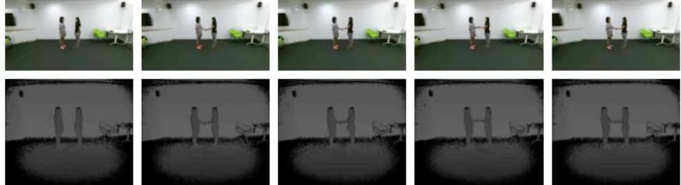
Figure 3.3: Example of RGB and depth frames from the NTU RGB+D Dataset.

sensor in 80 different viewpoints, and includes 40 subjects performing 60 distinct actions, including daily simple actions (e.g., brushing teeth, drinking, writing), interactions (e.g., kicking other person, hugging other person), and health-related actions (e.g., nausea or vomiting condition, sneeze/cough). We follow the two evaluation protocols originally proposed in [67], which are subject and cross-view. As in the original paper, we use about 5% of the training data as validation set for both protocols, in order to select the parametersλ,αandT. In this work, we use only RGB and depth data. The masked depth maps are converted to a three channel map via a jet mapping, as in [77].

3.3.2

Comparison with state of the art

Table 3.1 compares performances of different methods on the NTU RGB+D dataset. Classification accuracy is the standard performance measure used for this dataset: it is estimated according to the protocols (training and testing splits) reported in the respective works we are comparing with. The first part of the table (indicated by × symbol) refers to the unsupervised method proposed in [78], which achieve surprisingly high results even without relying on labels in learning representations. The second part refers to supervised methods (indicated by 4), divided according to the modalities used for training and testing. Here, we list the performance of the separate RGB and depth streams trained in step

(46)

3.3 Experiments

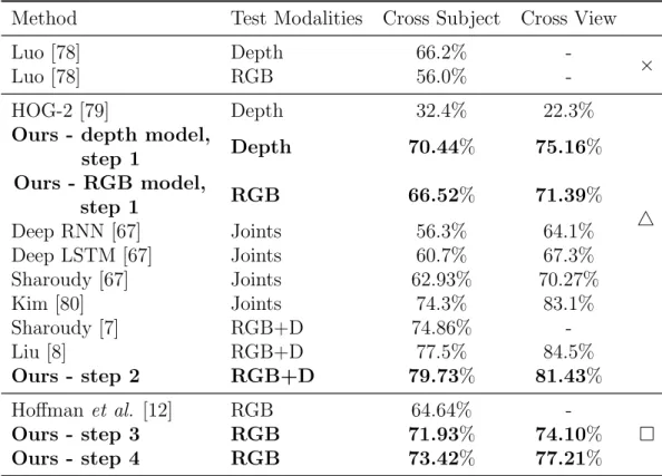
Method Test Modalities Cross Subject Cross View

Luo [78] Depth 66.2%

-×

Luo [78] RGB 56.0%

-HOG-2 [79] Depth 32.4% 22.3%

4

Ours - depth model,

step 1 Depth 70.44% 75.16% Ours - RGB model, step 1 RGB 66.52% 71.39% Deep RNN [67] Joints 56.3% 64.1% Deep LSTM [67] Joints 60.7% 67.3% Sharoudy [67] Joints 62.93% 70.27% Kim [80] Joints 74.3% 83.1% Sharoudy [7] RGB+D 74.86% -Liu [8] RGB+D 77.5% 84.5% Ours - step 2 RGB+D 79.73% 81.43% Hoffman et al. [12] RGB 64.64% Ours - step 3 RGB 71.93% 74.10% Ours - step 4 RGB 73.42% 77.21%

Table 3.1: Classification accuracies and comparisons with the state of the art. Performances referred to the several steps of our approach (ours) are highlighted in bold. ×refers to comparisons with unsupervised learning methods. 4refers to supervised methods: here train and test modalities coincide. refers to privileged information methods: here training exploits RGB+D data, while test relies on RGB data only.

1, as a reference. Of course, we expect our final model to perform better than the one trained on RGB only. We also propose our baseline, consisting in the teacher model trained in step 2. Its accuracy represents an upper bound for the final model, which will not rely on depth data at test time. The last part of the table (indicated by ) reports our model’s performances at 2 different stages together with the other privileged information method [12]. For both protocols, we can see that our privileged information approach outperforms [12], which is the only fair direct comparison we can make (same training & test data). Besides, as

(47)

ex-3.3 Experiments

pected, our final model performs better than “Ours - RGB model, step 1” since it exploits more data at training time, and worse than “Ours - step 2”, since it exploits less data at test time. Other RGB+D methods perform better (which is comprehensible since they rely on RGB+D in both training and test) but not by a large margin. More details and additional comments on the compared methods are provided in the supplementary material.

3.3.3

Ablation study

In this subsection, we discuss the results of the experiments carried out to under-stand the contribution of each part of the model and of the training procedure. Table 3.2 reports performances at the several training steps, different losses and model configurations.

Rows #1 and #2 refers to the first training step, where depth and RGB streams are trained separately. We can note that the depth stream network provides better performance with respect to the RGB one, as expected.

The second part of the table (Rows #3-5) shows the results using Hoffmanet al. ’s method [12],i.e. adopting a model initialized with the pre-trained networks from the first training step, and the hallucination network initialized using the depth network. Row #3 refers to the original paper [12] (i.e., using the lossLhall,

Eq. 3.3), and rows #4 and #5 refer to the training using the proposed lossesLGD

and L, in Eqs. 3.5 and 3.7, respectively. It can be noticed that the accuracies achieved using our proposed loss functions overcome that obtained in [12] by a significant margin (about 6% in the case of the total loss L).

The third part of the table reports performances after the training step 2. Rows #6 and #7 refer to the depth and RGB stream networks belonging to the model of row #8. This model corresponds to the architecture described in [1] and constitutes the upper bound for our hallucination model, since it uses RGB and

(48)

3.3 Experiments

# Method Test Modality Loss Cross-Subject Cross-View

1 Ours - step 1,

depth stream Depth x-entr 70.44% 75.16%

2 Ours - step 1,

RGB stream RGB x-entr 66.52% 71.39%

3 Hoffman [12]

w/o connections RGB eq. (3.3) 64.64%

-4 Hoffman [12]

-5 Hoffman [12]

-6 Ours - step 2,

7 Ours - step 2,

8 Ours - step 2 RGB & Depth x-entr 79.73% 81.43% 9 Ours - step 2

w/o connections RGB & Depth x-entr 78.27% 82.11%

10 Ours - step 3

w/o connections RGB (hall) eq. (3.3) 69.93% 70.64% 11 Ours - step 3

w/ connections RGB (hall) eq. (3.3) 70.47% -12 Ours - step 3

w/ connections RGB (hall) eq. (3.4) 71.52% -13 Ours - step 3

w/ connections RGB (hall) eq. (3.7) 71.93% 74.10% 14 Ours - step 3

w/o connections RGB (hall) eq. (3.7) 71.10% -15 Ours - step 4 RGB x-entr 73.42% 77.21%

Table 3.2: Ablation study. A full set of experiments is provided for cross-subject evaluation protocol, and for the cross-view protocol, only the most important results are reported.

depth for training and testing. Performances obtained by the model in row #8 and #9, with and without cross-stream connections, respectively, are the highest

(49)

3.3 Experiments

in absolute when using both modalities (around 78-79% for cross-subject and 81-82% for cross-view protocols, respectively), largely outperforming the accuracies obtained using only one modality (in rows #6 and #7).

The fourth part of the table (rows #10-14) shows results for our hallucination network after the several variations of learning processes, different losses and using or not using the cross-stream connections. One can note that the achieved performances when only RGB data are given in input, are in line with those achieved by the model fed by depth data. Depending on the variant adopted, accuracies are around 70-72%, reaching about 72% in the case of application of our full model before the fine-tuning step (row #14, cross-subject protocol). The depth stream model (in row #6) reaches 71%, whereas the model with both modalities in input (fixing the upper bound, row #8) reaches about 79%: only 6 percentage points separate the 2 models, showing the goodness of our proposed approach.

Finally, the last row, #15, reports results after the last fine-tuning step, which allows to reach the best accuracy with only the RGB modality as input, increasing the previous performance of about 1.5%, so narrowing the gap to the upper bound to about 4.5%.

Contribution of the cross-stream connections

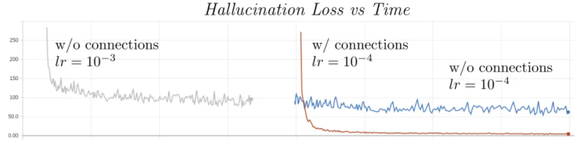
We claim that the signal injection provided by the cross-stream connections helps the learning of a better hallucination network. Row #13 and #14 show the per-formances for the hallucination network learning process, starting from the same point and using the same loss. The hallucination network that is learned using multiplicative connections performs better than its counterpart. This is illus-trated in figure 3.4: even after approximately half the number of iterations, the hallucination network learned with the multiplicative cross-stream connections is

(50)

3.3 Experiments w/o connections lr= 10−3 w/o connections lr= 10−4 w/ connections lr= 10−4

Hallucination Loss vs Time

Figure 3.4: The plot shows the hallucination loss Lhall of Eq. 3.3: the gray and

blue curves refers to the model where no multiplicative connections are used to learn the hallucination stream (row #14 of Table3.2). We started the experiment with learning rate set to 0.001, and continued after a while with learning rate set to 0.0001. The red curve shows instead Lhall after plugging the inter-stream

connections (row #13 of Table 3.2).

able to better minimize the Euclidean loss of Eq. 3.3.

Contributions of the proposed distillation loss (Eq. 3.7)

The distillation and Euclidean losses have complementary contributions to the learning of the hallucination network. This is observed by looking at the perfor-mances reported in rows #3, #4 and #5, and also #11, #12 and #13. Within both the training procedure proposed by Hoffmanet al. [12] and our staged train-ing process, the distillation loss improves over the Euclidean loss, and the com-bination of both improves over the rest. This suggests that both Euclidean and distillation losses have its own share and act differently to align the hallucination (student) and depth (teacher) feature maps and outputs’ distributions.

Contributions of the proposed training procedure

The intuition behind the staged training procedure proposed in this work can be ascribed to the dividi et impera (divide-and-conquer) strategy. In our case, it means breaking the problem in two parts: learning the actual task we aim to solve and learning the hallucination network to face test-time limitations. Row #5

(51)

3.3 Experiments

reports accuracy for the architecture proposed by Hoffman et al., and rows #15 report the performance for our model with connections. Both use the same loss to learn the hallucination network, and both start from the same initialization. We observe that our method outperform the one in row #5, which justifies the proposed staged training procedure.

Finally, we motivate for the use of the hallucination model in comparison with other naive approaches when dealing with missing or noisy modalities. Comparing rows #2 with #15, we further confirm (if still needed) that using the hallucination model is in fact more useful than training only with RGB data. We also observe that it is more useful to use our hallucination model than naively use totally corrupted depth data as input to the two-stream model. This is observed by comparing results in Table 3.3 and the performance at row #15 in Table 3.2. The following section studies with further detail the behavior of our model when tested using noisy depth data as input.

3.3.4

Inference with noisy depth

Suppose that in a real test case we can only access unreliable, i.e. noisy, depth data. Now the question is: how much we can trust such data? How better would it be to use a model in which depth is provided by an hallucination network, like that proposed in this work? In other words, we are finally interested in exploring how our model works under stress, and, more precisely, at which level of noise, hallucinating the depth modality becomes favorable with respect to using the full model with both input modalities (step 2).

The depth sensor used in the NTU dataset (Kinect), is an IR emitter coupled with an IR camera, and has very complex noise characterization comprising at least 6 different sources [81]. It is beyond the scope of this work to investigate noise models affecting the depth channel, so, for our analysis we choose the most

(52)

3.3 Experiments

σ2 _{no noise} ₁₀−3 ₁₀−2 ₁₀−1 ₁₀0 ₁₀1 _void Accuracy 81.43% 81.34% 81.12% 76.85% 62.47% 51.43% 14.24%

Table 3.3: Accuracy of the model tested with clean RGB and noisy depth data. Accuracy of the proposed hallucination model, i.e. with no depth at test time, is 77.21%.

commonly adopted noise model, i.e., the multiplicative speckle noise.

Hence, we inject multiplicative Gaussian noise in the depth image I in order to simulate speckle noise: I = I ∗n, n ∼ N(1, σ). Table 3.3 shows how perfor-mances of the network degrade when depth is corrupted with such Gaussian noise with increasing variance (cross-view protocol only). Results show that accuracy significantly decreases wrt the one guaranteed by our hallucination model (row #15 in Table 3.2), even with low noise variance. This means, in conclusion, that training an hallucination network is an effective way not only to obviate to the problem of a missing modality, but also to deal with noise affecting the input data channel.

3.3.5

Inverting the data modalities: RGB distillation

Despite the proposed architecture is general and can be applied to any multimodal pair of data streams, our model is not symmetric under the swap of the depth and RGB modalities. The connection between streams is engineered such that the RGB stream is fed with a signal coming from the depth stream, and not vice versa. The intuition for such choice of direction is that the depth stream learns from cleaner, more representative data (foreground depth maps), agnostic to texture, and is able to inform the RGB stream where the action is taking place, practically working as an augmentation tool for those regions of the feature map.

(53)

3.3 Experiments

In fact, the depth stream alone performs better the the RGB alone.

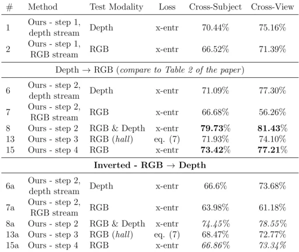
In [1], the authors tested different locations where to inject the optical flow signal, e.g. inside or outside the ResNet residual unit. Bi-directional connections were also investigated, i.e. both streams were injected one into the other. It was concluded that injecting signal into the optical flow stream decreases the model performance, and suggest that the reason can be ascribed to the RGB stream becoming dominant during training. We hypothesize that the same reasoning can be applied to the depth stream, which in our model takes the place of optical flow. In [1], the authors did not try to invert the connection, i.e. to inject signal from RGB to optical flow. We report the results of such experiment in Table 3.4. Line #8a reports the accuracy obtained by the teacher network at the end of step 2: not only such accuracy is lower than the one of our original teacher network (line #8), but also is only marginally higher than the one obtained by the final model (line #15), which only uses RGB at test time. Line # 8a represents thus a very poor upper bound (as compared to line # 8). This translates in a worse hallucination network (lines #13a) and worse distilled model (#15a).

3.3.6

Implementation details

Pre-processing & alignment

The multiplicative cross-stream connections present in our model require both RGB and depth frames to be spatially aligned, since they are element-wise operations over the feature maps. Such alignment comes for free when us-ing RGB and optical flow - which is computed directly from the appearance frames. However, this is not normally the case when using depth and RGB frames that are acquired with different sensors, and have different dimensions and aspect ratios as in the NTU RGB+D dataset, or other Kinect-acquired data. Fortunately, the NTU dataset provides the joints’ spatial coordinates in every

(54)

3.3 Experiments

# Method Test Modality Loss Cross-Subject Cross-View

1 Ours - step 1,

2 Ours - step 1,

Depth→ RGB (compare to Table 2 of the paper) 6 Ours - step 2,

7 Ours - step 2,

8 Ours - step 2 RGB & Depth x-entr 79.73% 81.43% 13 Ours - step 3 RGB (hall) eq. (7) 71.93% 74.10%

15 Ours - step 4 RGB x-entr 73.42% 77.21%

Inverted - RGB → Depth

6a Ours - step 2,

7a Ours - step 2,

8a Ours - step 2 RGB & Depth x-entr 74.45% 78.55% 13a Ours - step 3 RGB (hall) eq. (7) 68.47% 72.77%

15a Ours - step 4 RGB x-entr 66.86% 73.34%

Table 3.4: Inverting the cross-stream connection study. The last section of the table refers to results where the direction of the cross-stream connection has been inverted. The other results are also reported in the paper, as they refer to the model proposed.