2013
Modifications to classification and regression trees
to solve problems related to imperfect detection
and dependence
Mark McKelvey
Iowa State UniversityFollow this and additional works at:
https://lib.dr.iastate.edu/etd
Part of the
Statistics and Probability Commons
This Dissertation is brought to you for free and open access by the Iowa State University Capstones, Theses and Dissertations at Iowa State University Digital Repository. It has been accepted for inclusion in Graduate Theses and Dissertations by an authorized administrator of Iowa State University Digital Repository. For more information, please [email protected].
Recommended Citation
McKelvey, Mark, "Modifications to classification and regression trees to solve problems related to imperfect detection and dependence" (2013).Graduate Theses and Dissertations. 13523.
imperfect detection and dependence
by
Mark Wesley McKelvey
A dissertation submitted to the graduate faculty in partial fulfillment of the requirements for the degree of
DOCTOR OF PHILOSOPHY
Major: Statistics
Program of Study Committee: Philip Dixon, Major Professor
Petrutza Caragea Stephen Dinsmore
Heike Hofmann Daniel Nordman
Iowa State University Ames, Iowa
2013
DEDICATION
I would like to dedicate this thesis to my wife Beth and to my children without whose support I would not have been able to complete this work.
TABLE OF CONTENTS
LIST OF TABLES . . . vi
LIST OF FIGURES . . . viii
ACKNOWLEDGEMENTS . . . ix
ABSTRACT . . . x
CHAPTER 1. OVERVIEW . . . 1
1.1 Introduction . . . 1
CHAPTER 2. Incorporating Detection into Classification and Regression Trees for Occupancy Modeling . . . 5
2.1 Introduction . . . 5 2.1.1 Examples . . . 8 2.2 Methods . . . 9 2.2.1 Implementation . . . 10 2.3 Results . . . 11 2.3.1 Simulation Results . . . 11 2.3.2 Study Results . . . 13 2.4 Discussion . . . 17 2.5 Conclusion . . . 18 2.6 Literature Cited . . . 18
2.7 Extra material: R Code . . . 20
2.7.1 User Splits . . . 20
2.7.2 Companion functions . . . 26
2.7.4 Run code . . . 32
CHAPTER 3. Incorporating Dependence into Classification and Regression Trees for Occupancy Modeling . . . 40
3.1 Introduction . . . 40
3.1.1 Examples . . . 43
3.2 Methods . . . 44
3.2.1 Methods for Rats Example–dependence only . . . 44
3.2.2 Methods for Birds Example–dependence PLUS detection/occupancy . . 52
3.3 Results . . . 54
3.3.1 Results for Rats Example . . . 54
3.3.2 Results for Birds Example . . . 57
3.3.3 Simulation Evaluation of the Patchup Factor . . . 60
3.4 Discussion . . . 63
3.5 Literature Cited . . . 64
3.6 Extra material: R code for Unequal Variances method . . . 66
3.6.1 User splits . . . 66
3.6.2 Companion functions . . . 73
3.6.3 Proposed method each.parent . . . 76
3.6.4 Run code . . . 79
CHAPTER 4. Pruning Classification and Regression Trees with Modifica-tions for Occupancy Modeling . . . 82
4.1 Introduction . . . 82 4.2 Methods . . . 84 4.2.1 Implementation . . . 86 4.2.2 Simulated Scenarios . . . 86 4.3 Results . . . 89 4.4 Discussion . . . 95 4.4.1 Recommendations . . . 96
4.5 Conclusion . . . 97
4.6 Literature Cited . . . 98
4.7 Extra material: Detailed simulation results . . . 98
LIST OF TABLES
Table 2.1 Node estimates of occupancy and detection from the na¨ıve, orig.parent,
each.parent, and parent.v.2daughters methods. . . 14
Table 2.2 Node estimates of occupancy and detection from the p.v.d.v.d. method. 14 Table 2.3 AIC values computed using the plover data. . . 16
Table 2.4 Step-by-step AIC values for the orig.parent method. . . 16
Table 3.1 Node estimates from the clustered Rats example. . . 56
Table 3.2 Node estimates from the Rats example with independence. . . 56
Table 3.3 The node estimates of occupancy and detection for the Birds example resulting from the unequal variances, clustered method. . . 59
Table 3.4 The node estimates of occupancy and detection for the Birds example resulting from the unequal variances, independent method. . . 59
Table 3.5 Type I error rates for the Independent, equal variances, and unequal variances methods. . . 62
Table 4.1 Averaged results from a simulation using Design 1 with multiple levels of criteria C and D. . . 94
Table 4.2 Averaged results from a simulation using Design 2 with multiple levels of criteria C and D. . . 95
Table 4.3 The averaged results from a simulation using Design 1 with multiple levels of criterion A. . . 99
Table 4.4 The averaged results from a simulation using Design 2 with multiple levels of criterion A. . . 100
Table 4.5 The averaged results from a simulation using Design 1 with multiple
levels of criterion A and a constant level (zero) of criterion B. . . 102
Table 4.6 The averaged results from a simulation using Design 2 with multiple
levels of criterion A and a constant level (zero) of criterion B. . . 103
Table 4.7 The averaged results from a simulation using Design 1 with multiple
levels of criterion B. . . 105
Table 4.8 The averaged results from a simulation using Design 2 with multiple
LIST OF FIGURES
Figure 2.1 Trees produced from test1 and test2 simulations. . . 12
Figure 2.2 Comparing estimates of occupancy at each site between the 5 methods. 13
Figure 2.3 The tree produced using methods orig.parent, each.parent, and
par-ent.v.2daughters. . . 15
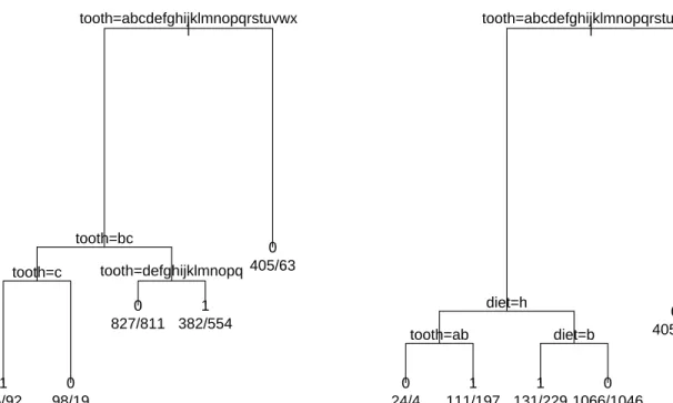
Figure 3.1 The tree structures produced by rpart() for the clustered and
indepen-dent approaches of the Rats example. . . 55
Figure 3.2 The tree structures produced by rpart() for the Birds example. . . 58
Figure 4.1 Two designs which assign occupancy probabilities to each patch during
the simulations. . . 89
Figure 4.2 The averaged results from simulations using Design 1 and Design 2 with
multiple levels of criterion A. . . 90
Figure 4.3 Comparison of the average number of pruning decisions resulting from
using only Criterion A versus using Criterion A with Criterion B equal to zero. . . 91
Figure 4.4 Comparison of the mean absolute errors resulting from pruning using
only Criterion A versus pruning using Criterion A with Criterion B equal to zero. . . 92
Figure 4.5 The averaged results from simulations using Design 1 and Design 2 with
ACKNOWLEDGEMENTS
I would like thank my major professor, Dr. Philip Dixon, for his guidance and infinite patience during this long, long journey of researching and writing my dissertation.
ABSTRACT
Classification and Regression Tree (CART) models provide a flexible way to model species’ habitat occupancy status, but standard CART algorithms have plenty of room for extensions. One such extension explores the survey error of imperfect detection. When an individual is not detected, that is often taken as sign of non-presence. However, the principle of imperfect detection tells us that just because one cannot find what they are looking for, that does not mean that what they are looking for is not present. We outline four methods for including de-tection probability in the process of growing the tree, and illustrate these methods using data from a study of mountain plovers (Dinsmore et al. 2003). The results depend on the method used to estimate detection and occupancy. For the mountain plover data, the tree structures produced by three of the methods are identical to that produced by the na¨ıve tree in which detection is ignored. The fourth method yields different splitting choices. Estimates of occu-pancy probability are consistently lower when using the na¨ıve tree than those computed using detection-adjusted trees. Accounting for imperfect detection is crucial even when occupancy is modeled using a CART tree.
In addition to imperfect detection, another extension to standard CART algorithms deals with spatial correlation. Many studies include a cluster-type sampling design where there is a clear spatial correlation between sampling locations. This correlation causes the variance of the node occupancy estimates in CART to be biased. We suggest a generalized estimating equa-tion (GEE)-based approach in which the na¨ıve variance estimates (calculated as if all locaequa-tions were independent) are “corrected” based on the data available in each parent node of the tree. The corrected variance estimates are then used to revise the binary-split decision criterion of the tree. The variances of each node in the split are assumed to be unequal. We demonstrate this method using data from a study on rats and also from a study on bird occurrences in Oregon.
When creating alternative methods of growing trees (i.e. how nodes are split) in CART, we expect to see [potentially] different trees. However, using those new methods also means that methodology involved in pruning the trees may need their own corresponding changes. For example, both of the types of methodology proposed above, incorporating imperfect detection and correlated data, led to an examination of current pruning criteria. Taking both of those new algorithms into account, we will discuss several pruning criteria that could be used in conjunction with our proposed CART methodology. We evaluated the performance of each criteria by using simulated examples for each criteria, which resulted in error rates that were used to assess the performance of the pruning criteria.
CHAPTER 1. OVERVIEW
1.1 Introduction
A classification and regression tree (CART) is a flexible alternative to logistic and linear regression models (De’ath and Fabricius 2000, Breiman et al. 1984). Unlike regression, CART can account for interactions in its binary tree structure because it does not require the as-sumption of additivity. CART allows the simultaneous use of both quantitative and qualitative covariates, makes no distributional assumptions, and is invariant to monotone transformations of variables (Breiman et al. 1984). Another advantage of CART is its ability to handle missing values. Whereas logistic regression would discard any individual with data missing from any one (or more) of the covariates, CART can still use that individual’s data to help formulate the model (Clark and Pregibon 1992, Harrell 2001, De’ath and Fabricius 2000, Breiman et al. 1984). These properties, along with its relative ease of construction and interpretation, have lead to widespread use of CART in ecology (e.g. Pesch et al 2011, Davidson et al 2010, Lehmann et al 2011, Maslo et al 2011).
CART creates a binary tree through recursive partitioning of the observations in the data set. A group of observations in the tree is called a “node”. At each single “parent” node in the tree, CART attempts to partition the data from the parent node into two more-homogeneous “daughter” nodes. CART uses an exhaustive processing algorithm that uses all of the covari-ates, checking every possible way to split the observations based on breaks in the covariate distributions.
Homogeneity of a node is often referred to as impurity. A measure of impurity is generally continuous and bounded on the lower end by zero, although it can be any formula which has a value to identify a perfectly homogeneous node (such as zero) and an increasing scale to
measure the relative strength of the split. A measure of zero indicates that no further splitting is required, while measures further from zero indicate an increasing propensity toward splitting. Impurity could also take the form of a statistical deviance (De’ath and Fabricius 2000, Clark and Pregibon 1992) when using a specific statistical model.
Some common measures of impurity for a classification tree (Breiman et al. 1984) are Entropy, Misclassification, Twoing and the Gini Index, which is often the default measure used for splitting in classification trees. When the responses are binary (yes / no), the Gini Index
defines impurity at a node withn observations as
(2×#Y es
n )∗(1− #Y es
n ) (1.1)
A calculated measure is used to rank each of the possible splits of a parent node. This measure is often based on a measure of impurity taken from each node in the triad (the parent node and two daughter nodes). In literature, this value might be referred to as a “decrease in impurity” or a “drop in deviance”. We also note that at times in the literature, “Deviance” appears to have referred to impurity in general, a specific function of impurity, or a statistical deviance based on a model. The combined impurity at the two daughter nodes is the sum of the impurity (e.g. the Gini Index) for each node. Then the decrease in impurity of the proposed split is defined as the difference between the impurity of the parent node and the combined impurity of the two daughter nodes. The proposed split with the largest decrease would be chosen for use in the tree.
When creating a CART model, the tree could potentially continue growing until every terminal node has only 1 observation in it. In order to avoid overfitting, CART employs several rules on when to stop growing the tree. The simplest of these rules is to stop splitting if the parent node in question is perfectly homogeneous with respect to the response variable.
Another very basic rule is that of node size. This constraint specifies the minimum parent node size required to even consider splitting, as well as setting the minimum daughter node size required to accept a proposed split. For example, it may be unreasonable to consider splitting a node with only 10 observations. Also, regardless of the homogeneity it may provide, splitting a node with 50 observations into a node with 48 observations and another with 2 observations
may not be statistically prudent.
Another stopping mechanism involves a choice of a value for the complexity parameter (cp). During tree construction, an estimated complexity value (cp*) is calculated for each potential split. If the estimated complexity cp* is not as large as the specified level (cp), then the split being considered is not made. The cp value can also be used post-tree formation to further prune the tree.
The user can also gain extra control through the definition of the measure of node impurity (node deviance) or through the calculation of the drop in deviance of potential splits. For classification modeling, the node deviance (D), along with the complexity parameter (cp), can be used together in a cost-complexity pruning algorithm. If
Dparent−
X
Dchild+cp
is not greater than zero for at least one set of splits below the parent node, then that initial split is not worth keeping at the current level of cp (Therneau and Atkinson 2011).
Of particular interest to this paper are uses of CART for occupancy modeling (e.g. De’ath
and Fabricius 2000; Bourg et al. 2005; Castell´on and Sieving 2006). It predicts occurrence or
abundance of a species using environmental covariates such as temperature, distance to water, and food availability. Occupancy modeling can be especially useful when the subject is difficult to find (due to mobility, concealment, or if the area being searched is very large in size), thus leading to scenarios with imperfect detection! It can also be used to predict occurrence in un-surveyed areas or potentially to understand the biological mechanisms. Sample data are often represented in clusters, which can cause issues with precision in model estimates.
This thesis addresses two main issues. The first issue being the application of CART to a set of occupancy data collected with the potential for imperfect detection. In order to build a classification (or regression) tree, a general assumption is that the identification status (or quantitative characteristic) of the individuals which you are using to create the tree are known, which then makes the internal calculations fairly straightforward. Modeling occupancy data with detection issues complicates this idea. If a status or characteristic value is uncertain,
that should change the creation process and interpretation of the CART tree. We will propose several methods as solutions to this problem.
The second issue involves any study in which the data were collected from clustered observa-tions. This violates another assumption of CART, which is that of independence. Independence is a highly sought-after commodity when collecting data, and is the default for many statis-tical methods. Without independence, we are left scrambling to compensate for the changes in variance that are sure to occur, and must adjust the modeling techniques accordingly. We propose a method that will adjust CART for the presence of correlated data.
Chapter 2 will focus on methods to solve the problem of using CART to model occupancy data with imperfect detection. Chapter 3 will be concerned with a proposal to adjust CART for the presence of correlated data. Chapter 4 presents a new way to think about evaluating and reducing CART trees to a manageable size in light of the methodology introduced in Chapters 2 and 3. Finally, Chapter 5 will summarize the findings of the previous three chapters.
CHAPTER 2. Incorporating Detection into Classification and Regression
Trees for Occupancy Modeling
Classification and Regression Tree (CART) models provide a flexible way to model species’ habitat occupancy status, but standard CART algorithms ignore imperfect detection. We out-line four methods for including detection probability in the process of growing the tree, and illustrate these methods using data from a study of mountain plovers (Dinsmore et al. 2003). The results depend on the method used to estimate detection and occupancy. The tree struc-tures produced by three of the methods are identical to that produced by the na¨ıve tree in which detection is ignored. The fourth method yields different splitting choices. Estimates of occu-pancy probability are consistently lower when using the na¨ıve tree than those computed using detection-adjusted trees. Accounting for imperfect detection is crucial even when occupancy is modeled using a CART tree.
2.1 Introduction
Occupancy modeling (OM) is a widely used tool among ecologists and wildlife researchers. It predicts occurrence or abundance of a species using environmental covariates, such as temper-ature, distance to water, and food availability. OM can be especially useful when the subject is difficult to find (due to mobility, concealment, or if the area being searched is very large in size). It can also be used to predict occurrence in un-surveyed areas or potentially to understand the biological mechanisms. Recent examples include predicting occupancy for the Siberian flying squirrel (Reunanen et al. 2002), describing the spatial population structure of the leaf-mining moth (Gripenberg et al. 2008), conservation planning for Finnish butterflies at different spatial scales (Cabeza et al. 2010), examining the role of habitat quality on chinook salmon spawning
(Isaak et al. 2007), and modeling nest-site occurrence for the Northern Spotted Owl (Stralberg et al. 2009).
A recent trend in OM research is to develop models that allow imperfect detection. With perfect detection, one model for occupancy at site i is a Bernoulli distribution,Yi ∼Bern(πi)
, where Yi = 1 if Seen (i.e. Detected) at site i, and πi = Prob(Occupancy) at site i =
f(X1, X2,· · ·Xk). The function f(X1, X2,· · · , Xk) relates Prob(occupancy) to the k environ-mental covariatesX1,X2,· · ·Xk. However, when detection is imperfect, i.e. Prob(Detect|Occupied)
= πd < 1, then πocc becomes partially masked by πd. A better model would be Yi ∼
Bern(πoccπd), The expected probabilities of observed data at a site on a given occasion are
then:
P(Y = 1) = probability of ‘Seen’ =πoccπd
P(Y = 0) = probability of ‘Not Seen’ = 1−πoccπd
= (1−πocc) +πocc(1−πd)
= P(Not there) +P(there but not seen)
Logistic regression is often used to predict occupancy probabilities. The logit function, log[πocc/(1−πocc)] relates occupancy probability to the environmental covariates.
log( πocc 1−πocc
) =β0+β1∗x1+...+βp∗xp
Failure to account for imperfect detection in logistic regression models is known to lead to biased estimates of occupancy probability (Tyre at al. 2003, Gu and Swihart 2004).
Logistic regression requires an explicit model for the influence of the environmental covari-ates. Commonly, the logistic regression model assumes linearity and additivity. The additivity assumption can be relaxed by including interaction terms, but without good knowledge of the appropriate interactions to include, this often leads to a large number of model terms and over-fitting (Hosmer and Lemeshow 2000).
A classification and regression tree (CART) is a flexible alternative to logistic classification models (De’ath and Fabricius 2000, Breiman et al. 1984). Unlike logistic regression, CART can account for interactions in its binary tree structure because it does not require the assumption of
additivity. CART allows the simultaneous use of both quantitative and qualitative covariates, makes no distributional assumptions, and is invariant to monotone transformations of variables (Breiman et al. 1984). Another advantage of CART is its ability to handle missing values. Whereas logistic regression would discard any individual with data missing from one of its covariates, CART can still use that individual’s data to help formulate the model (Clark and Pregibon 1992, Harrell 2001, De’ath and Fabricius 2000, Breiman et al. 1984). These properties, along with its relative ease of construction and interpretation, have lead to widespread use of
CART in occupancy modeling (e.g. De’ath and Fabricius 2000; Bourg et al. 2005; Castell´on
and Sieving 2006).
CART creates a binary tree by recursively paroning the observations in the data set. At each split, CART attempts to partition the data in a parent node into two more-homogeneous nodes. A calculated measure, often based on node impurity, is used to rank each of the possible splits of a parent node. Some common measures of node impurity for a classification tree (Brieman et al. 1984) are Entropy, Misclassification, Twoing, and the Gini index, which is often the default measure for splitting in a classification tree. When the responses are binary (yes / no), the
Gini Index defines impurity at a node withn observations as
(2×#Y es
n )∗(1− #Y es
n ) (2.1)
The combined deviance at the two daughter nodes is the sum of (2.1) for each node. Then
the calculated measure of the proposed split is defined as the drop in deviance from the parent node to the two combined daughter nodes. In general, a bigger change implies a better split.
However, the default use of a CART tree with seen/not seen data to model occupancy does not account for imperfect detection. Our goal is to modify the CART node-split We use a pair of simulated data sets and data on mountain plover sightings to illustrate our method. We present four methods for CART that incorporate detection probability into the tree-splitting process. Each method was evaluated using the same test data set and the results are compared. We present a measure (AIC) to evaluate the quality of the resulting tree. Our results from the mountain plover data suggest that using a single parameter to model detection probability within the whole tree is preferable.
2.1.1 Examples
2.1.1.1 Simulated Examples
We simulated two data sets in which the detection probability varied with environmental variables and their interaction. The Test1 data set has 3 variables. X3 is associated with detection probability, while X1 and X2 are associated with occupancy probability. The Test2 data set has 6 variables. X4 and X5 are associated with detection probability, variables X1, X2, X4, and X6 are associated with the occupancy probability, and X3 was irrelevant.
2.1.1.2 Plovers Example
Our motivating example is a multi-year study of Mountain Plovers in Montana, USA (Dins-more et al 2003). Mountain Plovers were searched for on prairie dog colonies during three sampling periods each year (20 May-10 June, 11-30 June, and 1-20 July) over a period of 13 years (1995-2007). During each search plovers were either seen (1) or not seen (0) on each prairie dog colony. There were a total of 81 colony sites involved in the survey, although not every site was sampled in every year. In 9 of the 13 years, some covariate information for each colony was collected simultaneously with the occupancy data. The covariates in the data set include the area of the prairie dog colony (AREA) and two colony shape metrics , a patch shape index (PSI) and a measure of perimeter-to-area ratio (PARA).
We removed the third sampling period in each year after exploratory analysis indicated that the detection probability in that period was substantially different from detection in the first two surveys. There is previous evidence for declining detection probabilities within each year (Dinsmore et al. 2003). We chose to work with the data from 2002. That year had a large number of sites visited twice (54) and a relatively low rate of na¨ıve detection (#ones over 2*#sites), thus the probability of misclassifying sites as ’non-occupied’ may be higher than in other years.
2.2 Methods
Taking a likelihood-based approach, we propose four possible approaches to incorporate
detection into a potential split from a parent node to two daughter nodes. We useπP,πL, and
πR to denote occupancy probabilities for the parent, left daughter, and right daughter nodes,
respectively. At each node, n0, n1 and n2 are the number of sites with no detections, one
detection or two detections. The four approaches are:
1. Separate detection and occupancy parameters (πd and πocc) at each node (6 total).
(This method is referred to as parent.v.daughter.v.daughter, or p.v.d.v.d.) The likelihood at each node in this situation is
L(πd, πocc|n0, n1, n2)∝[(1−πocc) +πocc(1−πd)2]n0∗[2πoccπd(1−πd)]n1 ∗[πoccπd2]n2
and the solutions to the score equations at a node are
ˆ πocc = n1+n2 (2πd−πd2)(n0+n1+n2) (2.2) ˆ πd = 2n2 2n2+n1 (2.3)
2. One detection parameter,πd, that applies to all 3 nodes (parent, left daughter and right
daughter), but 3 separate occupancy parameters (4 parameters total). We consider three estimators of πd:
(a) estimate πd from the root of the tree (all observations)and assume that detection
remains constant throughout the tree. (This method is referred to as orig.parent.)
(b) estimateπdfrom the parent node for each split, and assume that detection remains
constant only within that split.
(This method is referred to as each.parent.)
(c) estimate πd from the two proposed daughter nodes and assume that detection
(This method is referred to as parent.v.2daughters, or p.v.2d) The joint likelihood is
L(πd, πL, πR|n0L, n1L, n2L, n0R, n1R, n2R) ∝ [(1−πL) +πL(1−πd)2]n0L∗[2πLπd(1−πd)]n1L ∗[πLπd2]n2L∗[(1−πR) +πR(1−πd)2]n0R ∗[2πRπd(1−πd)]n1R ∗[πRπd2]n2R
Examining the solutions to the score equations ((2) and (3)), it can be seen that in the case when there are no ‘11’ sites (i.e.n2 = 0) and there is at least one ‘01’ or ‘10’ site (i.e.n1>0),
then ˆπd= 0 and ˆπocc =∞. There are other situations (not easily identifiable) when ˆπd∈[0,1] but ˆπocc >1. The use of optim() and a logit transformation of the probabilities prevents these situations, as well as preventing estimates of exactly 1 or exactly 0, which can cause errors in the calculation of the likelihoods.
For each method, the “drop in deviance” of a split takes the form of the test statistic of a Likelihood Ratio Test (LRT) between the parent node (same occupancy probability in all sites) and the two daughter nodes (two different occupancy probabilities). From all potential splits, the split with the largest test statistic is taken as the split used in the tree.
Akaike Information Criterion (AIC) is used as a measure of model selection between the
models produced from each of the four proposed methods. AIC is calculated as -2*l(θ) + 2k,
where l(θ) represents the maximized value of the Likelihood function based on the estimates
ˆ
πd = 0 and ˆπocc, and k is the number of parameters in the model. Models are penalized for
added complexity (additional parameters). Models with the lowest AIC values are generally preferred over other models.
2.2.1 Implementation
To obtain results using the na¨ıve method, which ignores the issue of detection, we combined the two sampling periods into one set (i.e. one “occasion”) of response data. We labeled each site with at least one ’1’ (i.e. ’11’, ’01’, or ’10’) as ’occupied’ and sites that had a ’00’ received a ’not-occupied’ designation. We then used the Gini Index as the measure of impurity to produce the na¨ıve tree.
For the imperfect detection methods, we replaced the Gini Index with a statistical deviance calculated using likelihood functions so that we could include a parameter for the detection probability. We maximized the log-likelihoods using the optim() function in R with the BFGS
method. The two parameters (πocc and πd) were estimated on the logistic scale and then the
results were back-transformed, thereby ensuring that our estimates fell within the parameter space (i.e. between 0 and 1) without having to truncate any estimates. Those estimated prob-abilities were then used to calculate the log-likelihood at each of the three nodes, which in turn was used to calculate the drop in deviance (in the form of a LRT) of the proposed split. This was done for every possible split from a parent node.
We performed the CART analyses with the rpart()function from in program R, which can
be found in the rpart package (Therneau and Atkinson 2010). We utilized the “user splits” option, which allows the creation and use of non-standard splitting functions and criteria.
2.3 Results
2.3.1 Simulation Results
From the test1 and test2 simulations, the best (using AIC) imperfect detection models were parent.v.2daughters (for test1) and the orig.parent model (for test2) method. We then compared the tree from the best models of each simulation to the trees produced assuming
perfect detection. Figure 2.1 displays these results. We show only the tops of the trees in an
effort to conserve space. The test1 trees show two differences in splits, in Nodes 2 (1st left-daughter node) and 13 (among the lower-right branches). The nodes in both trees split on the x1 variable, but do so in different places. For Node 2, this may only result in a small change
in estimated πocc, since the resulting nodes are still classified as “unoccupied”. However, for
Node 13, the change in estimated πocc, coupled with allowing πdet < 1, is enough to declare
the sites “occupied”. Between the test2 trees, we see only one structural difference, in Node 2, that has a similar effect as the Node 2 changes seen in the test1 trees.
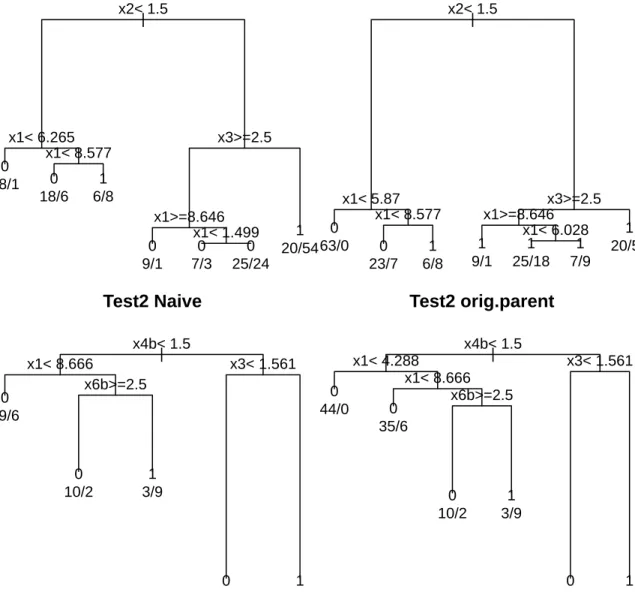
Test1 Naive
| x2< 1.5 x1< 6.265 x1< 8.577 x3>=2.5 x1>=8.646 x1< 1.499 0 68/1 0 18/6 1 6/8 0 9/1 0 7/3 0 25/24 1 20/54Test1 pv2d
| x2< 1.5 x1< 5.87 x1< 8.577 x3>=2.5 x1>=8.646 x1< 6.028 0 63/0 0 23/7 1 6/8 1 9/1 1 25/18 1 7/9 1 20/54Test2 Naive
| x4b< 1.5 x1< 8.666 x6b>=2.5 x3< 1.561 0 79/6 0 10/2 1 3/9 0 1Test2 orig.parent
| x4b< 1.5 x1< 4.288 x1< 8.666 x6b>=2.5 x3< 1.561 0 44/0 0 35/6 0 10/2 1 3/9 0 1Figure 2.1 Trees produced from the test1 and test2 simulations, comparing the na¨ıve method
to the imperfect detection methods parent.v.2daughters (test1) and orig.parent (test2). Both sets of trees display structural changes that can occur when ac-counting for imperfect detection. In the test1 trees, this occurs in Node 2 (the 1st left-daughter node) and Node 13 (among the lower-right branches). The test2 trees only reveal a structural difference in Node 2.
2.3.2 Study Results
From the analysis of the plover data, we see that site estimates of occupancy probability for
three of the proposed methods are quite similar (Figure2.2, Table2.1), but the fourth method,
p.v.d.v.d., produces very different estimates from the other methods (Table 2.2). The na¨ıve
method generally produces smaller estimates of occupancy probability than do the proposed methods. However, despite the estimates of occupancy and detection changing between meth-ods, the tree structure for all of the proposed methods except p.v.d.v.d. was identical to that of the na¨ıve tree (Figure2.3).
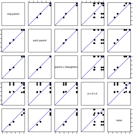
orig.parent 0.0 0.4 0.8 ● ● ● ● ● ● ● ● ● ● ● ● ● ● ● ● ● ● ● ● ● ● ● ● ● ● ● ● ● ● ● ● ● ● ● ● ● ● ● ● ● ● ● ● ● ● ● ● ● ● ● ● ● ● ● ● ● ● ● ● ●● ● ● ● ● ● ● ● ● ● ● ● ● ● ● ● ● ● ● ● ● ● ● ● ● ● ● ● ● ● ● ● ● ● ● ● ● ● ● ● ● ● ● ● ● ● ● 0.0 0.4 0.8 ● ● ● ● ● ●●● ● ● ● ● ● ● ● ● ● ● ● ● ● ● ● ● ● ● ● ● ● ● ● ● ● ● ● ● ● ● ● ● ● ● ● ● ● ● ● ● ● ● ● ● ● ● 0.0 0.4 0.8 ● ● ● ● ● ● ● ● ● ● ● ● ● ● ● ● ● ● ● ● ● ● ● ● ● ● ● ● ● ● ● ● ● ● ● ● ● ● ● ● ● ● ● ● ● ● ● ● ● ● ● ● ● ● 0.0 0.4 0.8 ● ● ● ● ● ● ● ● ● ● ● ● ● ● ● ● ● ● ● ● ● ● ● ● ● ●● ● ● ● ● ● ● ● ● ● ● ● ● ● ● ● ● ● ● ● ● ● ● ● ● ● ● ● each.parent ● ● ● ● ● ● ●● ● ● ● ● ● ● ● ● ● ● ● ● ● ● ● ● ●● ● ● ● ● ● ● ● ● ● ● ● ● ● ● ● ● ● ● ● ● ● ● ● ● ● ● ● ● ● ● ● ● ● ●●● ● ● ● ● ● ● ● ● ● ● ● ● ● ● ●● ● ● ● ● ● ● ● ● ● ● ● ● ● ● ● ● ● ● ● ● ● ● ● ● ● ● ● ● ● ● ● ● ● ● ● ● ● ● ● ● ● ● ● ● ● ● ● ● ● ● ● ● ● ● ●● ● ● ● ● ● ● ● ● ● ● ● ● ● ● ● ● ● ● ● ● ● ● ● ● ● ● ● ● ● ● ● ● ● ● ● ● ● ● ● ● ● ● ● ● ● ● ● ● ● ● ● ● ● ●● ● ● ● ● ● ● ● ● ● ● ● ● ● ● ● ● ● ● ● ● ● ● ● ● ● ● ● ● ● ● ● ● ● ● ● ● ● ● ● ● ● ● ● ● ● ● ● ● ● ● ● ● ● ● ● ● ● ● ● ● ● ● ● ● ● ● ● ● ● ● ● ● ● ● ● ● ● ● ● ● ● parent.v.2daughters ● ● ● ● ● ●●● ● ● ● ● ● ● ● ● ● ● ● ● ● ● ●● ● ● ● ● ● ● ● ● ● ● ● ● ● ● ● ● ● ● ● ● ● ● ● ● ● ● ● ● ● ● 0.0 0.4 0.8 ● ● ● ● ● ● ● ● ● ● ● ● ● ● ● ● ● ● ● ● ● ● ● ● ●● ● ● ● ● ● ● ● ● ● ● ● ● ● ● ● ● ● ● ● ● ● ● ● ● ● ● ● ● 0.0 0.4 0.8 ● ● ● ● ● ● ● ● ● ● ● ● ● ● ● ● ● ●● ● ● ● ● ● ● ● ● ● ● ● ● ● ● ● ● ● ● ● ● ● ● ● ● ● ● ● ● ● ● ● ● ● ● ● ● ● ● ● ● ● ● ● ● ● ● ● ● ● ● ● ● ●● ● ● ● ● ● ● ● ● ● ● ● ● ● ● ● ● ● ● ● ● ● ● ● ● ● ● ● ● ● ● ● ● ● ● ● ● ● ● ● ● ● ● ● ● ● ● ● ● ● ● ● ● ●● ● ● ● ● ● ● ● ● ● ● ● ● ● ● ● ● ● ● ● ● ● ● ● ● ● ● ● ● ● ● ● ● ● ● ● p.v.d.v.d. ● ● ● ● ● ● ● ● ● ● ● ● ● ● ● ● ● ●● ● ● ● ● ● ● ● ● ● ● ● ● ● ● ● ● ● ● ● ● ● ● ● ● ● ● ● ● ● ● ● ● ● ● ● 0.0 0.4 0.8 ● ● ● ● ● ● ● ● ● ● ● ● ● ● ● ● ● ● ● ● ● ● ●● ● ● ● ● ● ● ● ● ● ● ● ● ● ● ● ● ● ● ● ● ● ● ● ● ● ● ● ● ● ● ● ● ● ● ● ● ● ● ● ● ● ● ● ● ● ● ● ● ● ● ● ● ● ● ● ● ● ● ● ● ● ● ● ● ● ● ● ● ● ● ● ● ● ● ● ● ● ● ● ● ● ● ● ● 0.0 0.4 0.8 ● ● ● ● ● ● ● ● ● ● ● ● ● ● ● ● ● ● ● ● ● ● ● ● ● ● ● ● ● ● ● ● ● ● ● ● ● ● ● ● ● ● ● ● ● ● ● ● ● ● ● ● ● ● ● ● ● ● ● ● ● ● ● ● ● ● ● ● ● ● ● ● ● ● ● ● ● ● ● ● ● ● ● ● ● ● ● ● ● ● ● ● ● ● ● ● ● ● ● ● ● ● ● ● ● ● ● ● 0.0 0.4 0.8 0.0 0.4 0.8 naive
Figure 2.2 Comparing estimates of occupancy at each site between the 5 methods. The
straight lines have a slope of 1 and represent equality. Three of the proposed methods are quite similar (orig.parent, each.parent, and parent.v.2daughter), while the fourth proposed method produces very different estimates. The na¨ıve method generally produces smaller estimates of occupancy than the proposed imperfect detection methods do.
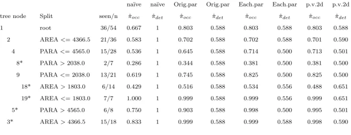
Table 2.1 The node estimates of occupancy and detection from the na¨ıve method, as well as from the proposed methods orig.parent (orig.par), each.parent (each.par), and par-ent.v.2daughters (p.v.2d). A (*) represents a terminal node of the tree. Note that while the tree structure is the same for each of these methods, the node estimates are very different from the na¨’ive method.
na¨ıve na¨ıve Orig.par Orig.par Each.par Each.par p.v.2d p.v.2d tree node Split seen/n πˆocc πˆdet ˆπocc πˆdet πˆocc πˆdet πˆocc πˆdet
1 root 36/54 0.667 1 0.803 0.588 0.803 0.588 0.803 0.588 2 AREA<= 4366.5 21/36 0.583 1 0.702 0.588 0.702 0.588 0.701 0.590 4 PARA<= 4565.0 15/28 0.536 1 0.645 0.588 0.714 0.500 0.713 0.501 8* PARA>2038.0 2/7 0.286 1 0.344 0.588 0.381 0.500 0.381 0.500 9 PARA<= 2038.0 13/21 0.619 1 0.745 0.588 0.825 0.500 0.825 0.500 18* AREA>1803.0 6/14 0.429 1 0.516 0.588 0.534 0.556 0.488 0.651 19* AREA<= 1803.0 7/7 1.000 1 0.999 0.588 0.999 0.556 0.999 0.651 5* PARA>4565.0 6/8 0.750 1 0.903 0.588 0.998 0.500 0.995 0.501 3* AREA>4366.5 15/18 0.833 1 0.999 0.588 0.999 0.588 0.998 0.590
Table 2.2 The node estimates of occupancy and detection resulting from the p.v.d.v.d.
method. A (*) represents a terminal node of the tree. While occupancy estimates
appear similar to those in Table 2.1, they should not be compared because of the
different tree structures.
tree node Split seen/n πˆocc ˆπdet
1 root 36/54 0.8028 0.5882 2* PSI>231 5/9 0.5926 0.7500 3 PSI<= 231 31/45 0.8560 0.5581 6* AREA<= 1261 4/8 0.5625 0.6667 7 AREA>1261 27/37 0.9250 0.5406 14 AREA<= 6103 19/26 0.9997 0.4617 28* AREA<= 2835 11/15 0.9998 0.4334 29* AREA>2835 8/11 0.9167 0.5454 15* AREA>6103 8/11 0.7682 0.7692
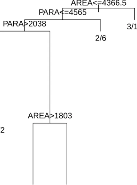
| AREA<=4366.5 PARA<=4565 PARA>2038 5/2 AREA>1803 8/6 0/7 2/6 3/15
Figure 2.3 The tree produced using methods orig.parent, each.parent, and
par-ent.v.2daughters, shown here, is identical to the na¨ıve tree produced without
ac-counting for imperfect detection. However, Table 2.1 displays the differences in
the parameter estimates, which show the advantage of the imperfect detection methods.
Based on the AIC values shown in Table 2.3, the best model for the plover data appears
to be the orig.parent model, which only estimates one detection probability parameter that is constant across all nodes (and thus all sites). Assuming a closed population, our original data clearly shows that the na¨ıve method is incorrect; any sites with observed data 0-1 or 1-0 (seen once, not seen once) indicate a need to account for imperfect detection.
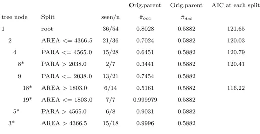
Table 2.4 shows the progression of AIC as we continue down the tree. Even though we
are adding one additional [occupancy] parameter at each split (one parent parameter becomes two daughter parameters), the AIC remains very similar until the final split, when it drops noticeably.
Table 2.3 AIC values computed using the plover data. AIC is calculated as -2*l(θ) + 2k. The best model is the orig.parent model.
Model AIC
Orig.parent 116.22
p.v.2d 121.15
Each.parent 121.93 p.v.d.v.d. 131.26
Table 2.4 The results from the proposed orig.parent method, along with AIC computed at
each split in the tree. Although the AIC calculation involves both leaves, the value is shown only for the left-daughter node of each split. A (*) represents a terminal node of the tree.
Orig.parent Orig.parent AIC at each split
tree node Split seen/n πˆocc πˆdet
1 root 36/54 0.8028 0.5882 121.65 2 AREA<= 4366.5 21/36 0.7024 0.5882 120.03 4 PARA<= 4565.0 15/28 0.6451 0.5882 120.79 8* PARA>2038.0 2/7 0.3441 0.5882 120.41 9 PARA<= 2038.0 13/21 0.7454 0.5882 18* AREA>1803.0 6/14 0.5161 0.5882 116.22 19* AREA<= 1803.0 7/7 0.999979 0.5882 5* PARA>4565.0 6/8 0.9031 0.5882 3* AREA>4366.5 15/18 0.9996 0.5882
2.4 Discussion
The simulated test1 and test2 data reveal that there can be structural changes caused by failing to account for imperfect detection when using CART, in addition to the less-visible (but still important) changes in parameter estimates at each node. Site classifications, using a cutoff
of πocc= 0.5, were changed from “unoccupied” to “occupied” designations.
The plover data, while an excellent real-world example of a situation where imperfect de-tection methodology should be applied, failed to lead to any structural differences between the na¨ıve tree and the trees for three of the four proposed methods. It is possible that similar detection probabilities throughout the tree, or the use of so few covariates, contributed to the lack of tree diversity.
The p.v.d.v.d. method classified all sites as being occupied (using a cutoff of πocc = 0.5). This seems very unusual, and you might think that allowing detection probabilities to change throughout the tree caused the tree structure to change. This is partially true, but allowing detection to differ at each node leads to erroneous use of the LRT. For the p.v.d.v.d. method, the LRT is a test of ANY difference between nodes (i.e. splitting decisions could be due to differences in detection and not just occupancy).
The idea of incorporating detection into classification and regression trees can be extended to random forests (Breiman 2001). Unfortunately, the random forest approach does not result in one final tree; it only reports an estimate for each individual, aggregated over all trees (the modal group for classification or the average for regression). A random forest would estimate
πocc for each site, averaged over a collection of trees, but it will not identify a single tree
structure. A single-tree CART approach may be more desirable due to its interpretability and ability to visually represent results (Prasad et al., 2006). Another CART extension that could benefit from using a detection parameter is boosted regression trees. Elith et al (2006), in their review of more than a dozen models for predicting species’ distributions from occurrence data, count boosted regression trees among the best models tested for various scenarios. These trees could still be improve by using detection to help estimate occupancy during the creation of each individual decision tree.
2.5 Conclusion
Classification and regression trees have proven their worth as an effective statistical model-ing tool for many situations. One area where they have previously lacked the ability to create an accurate model is in situations involving multiple surveys with imperfect detection. Being able to account for detection probability in the pursuit of predicting presence/absence of a desired individual (or characteristic, etc.) allows CART to be more accurate in its predictions. While they are by no means the final say in modifications to CART for detection, the four alternative methods presented here enable CART to be extended to statistical analyses which would otherwise use a different modeling tool.
2.6 Literature Cited
Bourg, Norman A., William J. McShea, Douglas E. Gill. 2005. Putting a CART Before the
Search: Successful Habitat Prediction for a Rare Forest Herb. Ecology. Vol. 86, No. 10, p.
2793-2804.
Breiman, L., Friedman, J., Olshen, R., and Stone, C. 1984. Classification and Regression Trees. Wadsworth International Group, Belmont, CA.
Breiman, Leo. 2001. Random Forests. Machine Learning. Vol. 45, p. 5-32.
Cabeza, Mar, Anni Arponen, Laura Jttel, Heini Kujala, Astrid van Teeffelen and Ilkka Hanski.
2010. Conservation planning with insects at three different spatial scales. Ecography. vol.
33, No. 1, p. 54-63.
Castell´on, Traci D., and Sieving, Kathryn E. 2006. Landscape History, Fragmentation, and
Patch Occupancy: Models for a Forest Bird with Limited Dispersal. Ecological Applications.
Vol. 16, No. 6, pp. 2223-2234.
Clark, L.A. and D. Pregibon. 1992. Chapter 9: Tree-based Models In: J.M. Chambers and
T.J. Hastie (eds.). Statistical Models in S. Wadsworth and Brooks, Pacific Grove, CA.
Davidson, T. A., Sayer, C. D., Langdon, P. G., Burgess, A. and Jackson, M. 2010. Inferring past zooplanktivorous fish and macrophyte density in a shallow lake: application of a new
regression tree model. Freshwater Biology Vol. 55, p. 584599.
De’ath, Glenn, and Fabricius, Katharina E. 2000. Classification and Regression Trees: A
Powerful Yet Simple Technique for Ecological Data Analysis. Ecology. Vol. 81, No. 11, pp.
3178-3192.
Dinsmore, Stephen J., Gary C. White, Fritz L. Knopf. 2003. Annual Survival and
Popu-lation Estimates of Mountain Plovers in Southern Phillips County, Montana. Ecological
Elith, J., Graham, C.H., Anderson, R.P., Dudk, M., Ferrier, S., Guisan, A., Hijmans, R.J., Huettmann, F., Leathwick, J.R., Lehmann, A., Lucia, J.L., Lohmann, G., Loiselle, B.A., Manion, G., Moritz, C., Nakamura, M., Nakazawa, Y., Overton, J.McC., Peterson, A.T., Phillips, S.J., Richardson, K., Scachetti-Pereira, R., Schapire, R.E., Sobero n, J., Williams, S., Wisz, M.S., and Zimmermann, N. 2006. Novel methods improve prediction of species
distributions from occurrence data. Ecography Vol. 29, p. 129155.
Gripenberg, Sofia, Otso Ovaskainen, Elly Morrin, and Tomas Roslin. 2008. Spatial population
structure of a specialist leaf-mining moth. Journal of Animal Ecology. Vol. 77, p. 757-767.
Gu, W. and Swihart, R.K. 2004. Absent or undetected? Effects of non-detection of species
occurrence on wildlife-habitat models. Biological Conservation vol. 116, p. 195-203.
Harrell, Frank. 2001. Regression modeling strategies: with applications to linear models, logistic regression, and survival analysis. Springer-Verlag, New York, NY.
Hosmer, David W. and Lemeshow, Stanley. 2000Applied Logistic Regression. John Wiley and
Sons, Inc., New York, NY.
Isaak, Daniel J., Russell F. Thurow, Bruce E. Rieman, Jason B. Dunham. 2007. Chinook Salmon Use of Spawning Patches: Relative Roles of Habitat Quality, Size, and Connectivity.
Ecological Applications. Vol. 17, No. 2, pp. 352-364.
Lehmann, C. E. R., Archibald, S. A., Hoffmann, W. A. and Bond, W. J. 2011. Deciphering
the distribution of the savanna biome. New Phytologist. Vol. 191, p. 197209.
Maslo, Brooke, Handel, Steven N. and Pover, Todd. 2011. Restoring Beaches for Atlantic Coast Piping Plovers (Charadrius melodus): A Classification and Regression Tree Analysis
of Nest-Site Selection. Restoration Ecology. Vol. 19, p. 194203.
Pesch, Roland, Gunther Schmidt, Winfried Schroeder, Inga Weustermann. 2011. Application
of CART in ecological landscape mapping: Two case studies. Ecological Indicators. Volume
11, No. 1, p. 115-122.
Prasad, A.M., L.R. Iverson and A. Liaw. 2006. Newer Classification and Regression Tree
Techniques: Bagging and Random Forests for Ecological Prediction. Ecosystems. Vol. 9,
No. 2, p. 181199.
Reunanen, Pasi, Ari Nikula, Mikko Mnkknen, Eija Hurme, Vesa Nivala. 2002. Predicting
Occupancy for the Siberian flying squirrel in old-growth forest patches. Ecological
Appli-cations. Vol. 12, No. 4, pp. 1188-1198.
Stralberg, Diana, Katherine E. Fehring, Lars Y. Pomara, Nadav Nur, Dawn B. Adams, Daphne
Hatch, Geoffrey R. Geupel, Sarah Allen. 2009. Modeling nest-site occurrence for the
Northern Spotted Owl at its southern range limit in central California. Landscape and
Therneau, Terry and Atkinson, Elizabeth. R port by Brian Ripley. 2010. rpart: Recursive Partitioning. R package version 3.1.-46.
http://CRAN.R-project.org/package=rpart
Tyre, A.J., Tenhumberg, B., Field, S.A., Niejalke, D., Parris, K., and Possingham, H.P. 2003. Improving precision and reducing bias in biological surveys: estimating false-negative error rates. Ecological Applications. vol. 13, p. 1790-1801.
2.7 Extra material: R Code
2.7.1 User Splits
# Mark McKelvey attempting to use the "user splits" option in R # Requires 3 pieces: Init, Eval, and Splits
# Optional 4th part called ’parms’ to pass in other information
# *NOTE: parms MUST be part of the call to rpart().
# It will not work from the global environment.
# I also change init$functions$print and init$functions$text
options(warn = 1) #prints warnings as they occur, # rather than waiting until the end
options(digits=4) # controls number of digits/decimals (default is 7) # if digits is set too low, numbers may go to # scientific notation
library(rpart) set.seed(7)
################################################################ # The ’evaluation’ function. Called once per node.
# Produce a label (1 or more elements long) for labeling each node, # and a deviance. The latter is
# - of length 1
# - equal to 0 if the node is "pure" in some sense (unsplittable) # - does not need to be a deviance: any measure that gets larger # as the node is less acceptable is fine.
# - the measure underlies cost-complexity pruning, however ###############
############### Mark’s eval() code temp1 <- function(y, wt, parms) {
print("***** START: Evaluating *****") Ns <- timesseen(y);
# NOTE: Ns[1] = n0 = never seen, Ns[2] = n1 = seen once, # Ns[3] = n2 = seen twice...
# If using orig.parent, I’d like to report the same prob.det
# being used in the split function; also the corresponding prob.occ if(parms$mygoodness==1){ param.parent <- optim(c(0.5), lnl.t.fixed,
gr=NULL, method="BFGS", control=list(fnscale=-1), prob.det = parms$prob.det, Ns = Ns )$par
param.parent <- backt(param.parent) prob.occ <- param.parent[1]
prob.det <- parms$prob.det }
# Anything else, I will report the node-specific prob.det and prob.occ # Note that for each.parent and p.v.2d methods, this does not reflect # the values being used in the split() function
else{
param.parent <- optim(c(0.5, 0.5), lnl.t, gr=NULL, method="BFGS", control=list(fnscale=-1), Ns=Ns )$par
param.parent <- backt(param.parent) prob.occ <- param.parent[1]
prob.det <- param.parent[2] }
labels <- matrix(nrow=1, ncol=5) # labels[1] is the fitted y category
# labels[2] is sum(y == 0) i.e. the "unseen" sites # labels[3] is sum(y >= 1) i.e. the "seen" sites # labels[4] is prob.occ
# labels[5] is prob.det
labels[1] <- ifelse(prob.occ >= parms$cutoff, 1, 0) labels[2] <- Ns[1]
labels[3] <- sum(Ns[-1]) labels[4] <- prob.occ labels[5] <- prob.det print(labels)
dev <- ifelse(prob.occ >= parms$cutoff, Ns[1], sum(Ns[-1])) ret <- list(label=labels, deviance=dev)
print("***** END: Evaluating *****") ret
}
############### end Mark’s eval() code ###############
# The split function, where most of the work occurs. # Called once per split variable per node.
# If continuous=T
# The actual x variable is ordered
# y is supplied in the sort order of x, with no missings, # return two vectors of length (n-1):
# goodness = goodness of the split, larger numbers are better.
# 0 = couldn’t find any worthwhile split
# the ith value of goodness evaluates splitting obs 1:i vs (i+1):n # direction= -1 = send "y< cutpoint" to the left side of the tree # 1 = send "y< cutpoint" to the right
# this is not a big deal, but making larger "mean y’s" move towards # the right of the tree, as we do here, seems to make it easier to
# read
# If continuous=F, x is a set of values defining the groups for an # unordered predictor. In this case:
# direction = a vector of length m= "# groups".
# direction actually displays the names/labels for each group. # It asserts that the best split can be found by
# lining the groups up in this order and going from left to right, # so that only m-1 splits need to be evaluated rather than 2^(m-1) # goodness = m-1 values here.
#
# The reason for returning a vector of goodness is that the C routine # enforces the "minbucket" constraint. It selects the best return value # that is not too close to an edge.
###############
############### Mark’s split() code
temp2 <- function(y, wt, x, parms, continuous) { #print("***** START: Splitting *****")
if(parms$mygoodness==1){mygoodness=LRT.orig.parent} if(parms$mygoodness==2){mygoodness=LRT.each.parent}
if(parms$mygoodness==3){mygoodness=LRT.parent.v.2daughters}
if(parms$mygoodness==4){mygoodness=LRT.parent.v.daughter.v.daughter} idx <- order(x); x <- x[idx]; y <- y[idx,];
#Just in case ordering is not already done elsewhere y <- cbind(y)
# If y is a vector, this allows me to calculate n using only one method n <- nrow(y)
parent <- y # In my code, the node being split is called the parent if (continuous) { # continuous x variable
# Get the goodness
## MAKE SURE IT IS A VECTOR!!
## Because rpart does the min. node size requirements elsewhere, ## I just have to compute n-1 deviances here.
possibles <- rep(0,n-1) direction <- rep(-1, n-1)
prob.occ.L = prob.occ.R <- rep(0, n-1) for (i in 1:(n-1)) {
left <- matrix(parent[1:i,], ncol=ncol(parent)) right <- matrix(parent[(i+1):n,], ncol=ncol(parent)) if(x[i]==x[i+1]) {next}
### NOT allowed to split up observations with the same x value info <- mygoodness(parent, left, right, orig.prob.det=parms$prob.det)
possibles[i] <- info[1] # test stat. for a likelihood ratio test prob.occ.L[i] <- info[2]
prob.occ.R[i] <- info[3]
# Get the direction ALSO A VECTOR!!
if(prob.occ.L[i] > prob.occ.R[i]){ direction[i] <- 1}
# Compares occupancy probabilities, sends the higher one to the right } # end ’for’ loop
goodness <- possibles
ret <- list(goodness=goodness, direction=direction) #print("***** END: Splitting *****")
ret } else {
# Categorical X variable
# we can order the categories by their means # (i.e. estimated prob.occ values)
# then use the same code as for a non-categorical ux <- sort(unique(x))
# Sort does smallest to largest (either numerical or alphabetical) m <- length(ux)
occs <- 0 for(i in 1:m){
group <- y[x==ux[i], ] Ns <- timesseen(group);
param <- optim(c(0.5, 0.5), lnl.t, gr=NULL, method="BFGS",
control=list(fnscale=-1), Ns=Ns )$par param <- backt(param)
prob.occ <- param[1] occs[i] <- prob.occ
} # end ’i’ loop
ord <- order(occs) #tells where each number belongs in order # e.g. 2 1 4 3 means that the first number is second-lowest,
# Get the goodness
## MAKE SURE IT IS A VECTOR!!
## Because rpart does the minimum node size elsewhere, ## I just have to compute m-1 deviances here.
possibles <- rep(0,m-1)
prob.occ.L = prob.occ.R <- rep(0, m-1) for (i in 1:(m-1)) {
left <- parent[ x<=ux[i], ] right <- parent[ x>ux[i], ]
info <- mygoodness(parent, left, right, orig.prob.det=parms$prob.det) possibles[i] <- info[1]
prob.occ.L[i] <- info[2] prob.occ.R[i] <- info[3] } # Get the direction ALSO A VECTOR!!
direction <- ux[ord] goodness <- possibles
ret <- list(goodness=goodness, direction=direction) #print("***** END: Splitting *****")
ret }
}
############### end Mark’s split() code ###############
# The init function:
# fix up y to deal with offsets
# return a parms list--this can be passed in from the call to rpart(), # but it MUST be reproduced (or changed) in init()
# parms includes cutoff (for predictions/labeling),
# occasions (# sampling times),
# prob.det (if specified by the user), and
# goodness (which imperfect detection method is used) # numresp is the number of values produced by the eval routine’s "label" # numy is the number of columns for y
# summary is a function used to print one line in summary.rpart # yval is the matrix "yval2" in tree$frame
# each row contains predicted value, deviance, n, prob.occ, prob.det # text is a function used to put text on the plot in text.rpart
# *NOTE: The split information printed is NOT controlled by the text
# function in init()
# In general, this function would also check for bad data, see # rpart.poisson for example
###############
############### begin Mark’s init() code temp3 <- function(y, offset, parms, wt) {
print("***** START: Init *****") if (!is.null(offset)) y <- y-offset
# IF method is orig.parent and prob.det is not specified: if(parms$mygoodness==1 & is.null(parms$prob.det)==TRUE) { # Calculate orig.prob.det from the very first parent node # (i.e. all of the data)
Ns <- timesseen(y)
param.parent <- optim(c(0.5, 0.5), lnl.t, gr=NULL, method="BFGS", control=list(fnscale=-1), Ns = Ns)$par param.parent <- backt(param.parent)
#orig.prob.occ <- param.parent[1] orig.prob.det <- param.parent[2] parms$prob.det <- orig.prob.det
} # end ’if’ statement
ret <- list(y=y, parms=parms, numresp=5, numy=parms$occasions, summary= function(yval, dev, wt, ylevel, digits ) {
paste("predicted value=", yval[,1], "deviance=", dev, "prob.occ=", round(yval[,4],digits), "prob.det=", round(yval[,5],digits) )
}, #end summary
text= function(yval, dev, wt, ylevel, digits, n, use.n ) { nclass <- (ncol(yval) - 1)/2
group <- yval[, 1]
counts <- yval[, 1 + (1:nclass)]
if (!is.null(ylevel)) {group <- ylevel[group] } temp1 <- format(counts, digits)
if (nclass > 1) { temp1 <- apply(matrix(temp1,
ncol = nclass), 1, paste, collapse = "/") } if (use.n) { out <- paste(format(group,
justify = "left"), "\n", temp1, sep = "") } else {out <- format(group, justify = "left") }
return(out)
}, #end text print= function(yval, ylevel, digits){
if (is.null(ylevel)) {temp <- as.character(yval[, 1]) } else {temp <- ylevel[yval[, 1]] }
if (nclass < 5) {yprob <- format(yval[, 1 + nclass + 1:nclass], digits = digits, nsmall = digits)}
else {yprob <- formatg(yval[, 1 + nclass + 1:nclass], digits = 2)} if (is.null(dim(yprob))) {yprob <- matrix(yprob, ncol = length(yprob)) }
temp <- paste(temp, " (", yprob[, 1], sep = "")
for (i in 2:ncol(yprob)) temp <- paste(temp, yprob[, i], sep = " ") temp <- paste(temp, ")", sep = "")
temp
} #end print ) # end ret
print("***** END: Init *****") ret
}
2.7.2 Companion functions
# Calculates the total number of times the species was detected at each site timesseen <- function(y){ timesseen <- 0 Ns <- rep(0, (ncol(y)+1) ) for (i in 1:nrow(y)){ timesseen[i] <- sum(y[i, ]) } for (j in 1:length(Ns)){ Ns[j] <- sum(timesseen==(j-1)) }
# NOTE: Ns[1] = n0 = never seen, Ns[2] = n1 = seen once, # Ns[3] = n2 = seen twice
return(Ns) } #end timesseen
# backtransforming parameters when using logistic representation backt <- function(ln.param) {
1/(1+exp(-ln.param)) } #end backt ###########
# lnl using logistic parameterization
# Used for any node when estimating both prob.occ and prob.det lnl.t <- function(param, Ns){ ln.Likelihood(backt(param), Ns) } #end lnl.t ln.Likelihood <- function(x, Ns){ prob.occ <- x[1] prob.det <- x[2]
k <- length(Ns)-1 # k = number of sampling occasions ln.like <- Ns[1]*log((1-prob.occ) + prob.occ*(1-prob.det)^k)
for(i in 1:k){ # occupied, seen ’i’ times out of ’k’ possible ln.like <- ln.like + Ns[i+1]*log( choose(k,i) * prob.occ * (prob.det^i) *
((1-prob.det)^(k-i)) ) } # end ’i’ loop
return(ln.like) } #end ln.Likelihood ###########
# Need for nodes when I’m fixing prob.det while optimizing pi.occ # this occurs in orig.parent and each.parent
lnl.t.fixed <- function(param, prob.det, Ns){
ln.Likelihood.fixed(backt(param), prob.det, Ns) } #end lnl.t.fixed
ln.Likelihood.fixed <- function(x, prob.det, Ns){ prob.occ <- x[1]
k <- length(Ns)-1 # k = number of sampling occasions
ln.like <- Ns[1]*log((1-prob.occ) + prob.occ*(1-prob.det)^k) # not occupied or occupied and seen 0 times
for(i in 1:k){ # occupied, seen ’i’ times out of ’k’ possible ln.like <- ln.like + Ns[i+1]*log( choose(k,i) * prob.occ * (prob.det^i) *
((1-prob.det)^(k-i)) ) } # end ’i’ loop
return(ln.like) } #end ln.Likelihood ###########
# lnl for parent.v.2daughters
lnl.star.t <- function(param, Ns.left, Ns.right){
ln.Likelihood.STAR2(backt(param), Ns.left, Ns.right) } #end lnl.star.t
# lnl for parent.v.2daughters
ln.Likelihood.STAR2 <- function(x, Ns.left, Ns.right){
prob.occ.L <- (x[1]); prob.occ.R <- (x[2]); prob.det.star <- (x[3]); k <- length(Ns.left)-1 # k = number of sampling occasions
ln.like <- Ns.left[1]*log((1-prob.occ.L) + prob.occ.L*(1-prob.det.star)^k) + Ns.right[1]*log((1-prob.occ.R) + prob.occ.R*(1-prob.det.star)^k )
for(i in 1:k){ # occupied, seen ’i’ times out of ’k’ possible ln.like <- ln.like + Ns.left[i+1]*log( choose(k,i) * prob.occ.L *
(prob.det.star^i) * ((1-prob.det.star)^(k-i)) ) + Ns.right[i+1]*log( choose(k,i) * prob.occ.R * (prob.det.star^i) * ((1-prob.det.star)^(k-i)) ) } # end ’i’ loop
########### ##############
############## The following two functions are needed to label
# my print output properly
print.rpart <- function(x, minlength=0, spaces=2, cp, digits=getOption("digits"), ...) {
if(!inherits(x, "rpart")) stop("Not legitimate rpart object")
if (!is.null(x$frame$splits)) x <- rpconvert(x) #help for old objects if (!missing(cp)) x <- prune.rpart(x, cp=cp)
frame <- x$frame
ylevel <- attr(x, "ylevels")
node <- as.numeric(row.names(frame)) depth <- tree.depth(node)
indent <- paste(rep(" ", spaces * 32), collapse = "") #32 is the maximal depth
if(length(node) > 1) {
indent <- substring(indent, 1, spaces * seq(depth))
indent <- paste(c("", indent[depth]), format(node), ")", sep = "") }
else indent <- paste(format(node), ")", sep = "") tfun <- (x$functions)$print
if (!is.null(tfun)) { if (is.null(frame$yval2))
yval <- tfun(frame$yval, ylevel, digits)
else yval <- tfun(frame$yval2, ylevel, digits) }
else yval <- format(signif(frame$yval, digits = digits)) term <- rep(" ", length(depth))
term[frame$var == "<leaf>"] <- "*"
z <- labels(x, digits=digits, minlength=minlength, ...) n <- frame$n
z <- paste(indent, z, n, format(signif(frame$dev, digits = digits)), yval, term)
omit <- x$na.action if (length(omit))
cat("n=", n[1], " (", naprint(omit), ")\n\n", sep="") else cat("n=", n[1], "\n\n")
#This is stolen, unabashedly, from print.tree if (x$method=="class")
cat("node), split, n, loss, yval, (yprob)\n") # NEW PART!!!
if (x$method=="user"){ cat("node), split, n, deviance, yval, prob.occ, prob.det\n") }
#####
else cat("node), split, n, deviance, yval\n") cat(" * denotes terminal node\n\n") cat(z, sep = "\n")
return(invisible(x)) #end of the theft }
# This one is located in treemisc.R tree.depth <- function(nodes)
{
depth <- floor(log(nodes, base = 2) + 1e-7) as.vector(depth - min(depth))
}
2.7.3 Four Proposed Methods
LRT.orig.parent <- function(parent, left, right, orig.prob.det){ # PARENT Ns.parent <- timesseen(parent) # for example, n0 <- Ns[1]; n1 <- Ns[2]; n2 <- Ns[3]; ... # LEFT Ns.left <- timesseen(left) # RIGHT Ns.right <- timesseen(right)
param.parent <- optim(c(0.5), lnl.t.fixed, gr=NULL, method="BFGS", control=list(fnscale=-1), prob.det = orig.prob.det,
Ns = Ns.parent )$par
param.parent <- backt(param.parent) prob.occ <- param.parent[1]
param.left <- optim(c(0.5), lnl.t.fixed, gr=NULL, method="BFGS", control=list(fnscale=-1), prob.det = orig.prob.det,
Ns=Ns.left)$par param.left <- backt(param.left) prob.occ.L <- param.left[1]
param.right <- optim(c(0.5), lnl.t.fixed, gr=NULL, method="BFGS", control=list(fnscale=-1), prob.det = orig.prob.det,
Ns=Ns.right)$par
prob.occ.R <- param.right[1]
upper <- ln.Likelihood(c(prob.occ, orig.prob.det), Ns.left) + ln.Likelihood(c(prob.occ, orig.prob.det), Ns.right) lower <- ln.Likelihood(c(prob.occ.L, orig.prob.det), Ns.left) +
ln.Likelihood(c(prob.occ.R, orig.prob.det), Ns.right) test.stat <- -2*(upper-lower)
out <- c(test.stat, prob.occ.L, prob.occ.R, orig.prob.det) return(out) }
LRT.each.parent <- function(parent, left, right, orig.prob.det){ # LEFT
Ns.left <- timesseen(left) # RIGHT
Ns.right <- timesseen(right)
param.parent <- optim(c(0.5, 0.5), lnl.t, gr=NULL, method="BFGS", control=list(fnscale=-1),Ns = (Ns.left+Ns.right) )$par param.parent <- backt(param.parent)
prob.occ <- param.parent[1] prob.det <- param.parent[2]
param.left <- optim(c(0.5), lnl.t.fixed, gr=NULL, method="BFGS", control=list(fnscale=-1), prob.det = prob.det, Ns=Ns.left)$par
param.left <- backt(param.left) prob.occ.L <- param.left[1]
param.right <- optim(c(0.5), lnl.t.fixed, gr=NULL, method="BFGS", control=list(fnscale=-1), prob.det = prob.det, Ns=Ns.right)$par param.right <- backt(param.right)
prob.occ.R <- param.right[1]
upper <- ln.Likelihood(c(prob.occ, prob.det), Ns.left) + ln.Likelihood(c(prob.occ, prob.det), Ns.right) lower <- ln.Likelihood(c(prob.occ.L, prob.det), Ns.left) +
ln.Likelihood(c(prob.occ.R, prob.det), Ns.right) test.stat <- -2*(upper-lower)
out <- c(test.stat, prob.occ.L, prob.occ.R, prob.det) return(out) }
LRT.parent.v.daughter.v.daughter <- function(parent, left, right, orig.prob.det){ # LEFT
# RIGHT
Ns.right <- timesseen(right)
param.parent <- optim(c(0.5, 0.5), lnl.t, gr=NULL, method="BFGS", control=list(fnscale=-1), Ns= (Ns.left + Ns.right) )$par param.parent <- backt(param.parent)
prob.occP <- param.parent[1] prob.detP <- param.parent[2]
param.left <- optim(c(0.5, 0.5), lnl.t, gr=NULL, method="BFGS", control=list(fnscale=-1), Ns=Ns.left )$par
param.left <- backt(param.left) prob.occ.L <- param.left[1] prob.det.L <- param.left[2]
param.right <- optim(c(0.5, 0.5), lnl.t, gr=NULL, method="BFGS", control=list(fnscale=-1), Ns=Ns.right )$par
param.right <- backt(param.right) prob.occ.R <- param.right[1] prob.det.R <- param.right[2]
upper <- ln.Likelihood(c(prob.occP, prob.det.L), Ns.left) + ln.Likelihood(c(prob.occP, prob.det.R), Ns.right) lower <- ln.Likelihood(c(prob.occ.L, prob.det.L), Ns.left) +
ln.Likelihood(c(prob.occ.R, prob.det.R), Ns.right) test.stat <- -2*(upper-lower)
out <- c(test.stat, prob.occ.L, prob.occ.R, prob.det.L, prob.det.R) return(out) }
LRT.parent.v.2daughters<-function(parent, left, right, orig.prob.det){ # LEFT
Ns.left <- timesseen(left) #RIGHT
Ns.right <- timesseen(right)
param.parent <- optim(c(0.5, 0.5), lnl.t, gr=NULL, method="BFGS", control=list(fnscale=-1), Ns = (Ns.left + Ns.right) )$par
param.parent <- backt(param.parent) prob.occ.P <- param.parent[1]
prob.det.P <- param.parent[2]
param.star <- optim(c(0.5, 0.5, 0.5), lnl.star.t, gr=NULL, method="BFGS", control=list(fnscale=-1), Ns.left=Ns.left,
Ns.right=Ns.right)$par param.star <- backt(param.star)
pi.L <- param.star[1]; pi.R <- param.star[2];
prob.det.star <- param.star[3]
param.upper <- c(prob.occ.P, prob.occ.P, prob.det.star) param.lower <- c(pi.L, pi.R, prob.det.star)
upper <- ln.Likelihood.STAR2(param.upper, Ns.left, Ns.right) lower <- ln.Likelihood.STAR2(param.lower, Ns.left, Ns.right) test.stat <- -2*(upper-lower)
out <- c(test.stat, param.lower) return(out) }
2.7.4 Run code
#Mark McKelvey
plovers <- read.csv("C://Documents and Settings/Owner/My Documents/ Research Part I/McKelvey data.csv", header=T)
attach(plovers) library(rpart);
########################### ###########################
X2002 <- 0
for (i in 1:81) { X2002[i] <- sum(X2002.1[i] + X2002.2[i])
ifelse(X2002[i]>=1, X2002[i] <- 1, X2002[i] <- 0) } data.2002 <- data.frame(X2002, A02, X02PARA, X02PSI)
#for matching with rpart
colnames(data.2002) <- c("X2002", "AREA", "PARA", "PSI") doubledown <- cbind(X2002, X2002, A02, X02PARA, X02PSI)
#### REMINDER: FOR my personal (self-written) optim 4 code, completedata.2002 NEEDS TO BE A MATRIX #### THE DATA FRAME IS NEEDED FOR USER.SPLITS
completedata.mat.2002 <- cbind(X2002.1, X2002.2, A02, X02PARA, X02PSI) #for incorporating detection
colnames(completedata.mat.2002) <- c("X2002.1", "X2002.2", "AREA", "PARA", "PSI") completedata.df.2002 <- as.data.frame(completedata.mat.2002) detach(plovers)
######################################## ######################################## #Source code progression:
#source("C://Documents and Settings/Owner/My Documents/Research Part I/ MY rpart functions with Optim 4.R")