Optimizing Offloading Strategies
in Mobile Cloud Computing
Esa Hyyti¨a
Department of Communications and Networking, Aalto University
Finland
Thrasyvoulos Spyropoulos
Department of Mobile CommunicationsEURECOM, Sophia-Antipolis France
J¨org Ott
Department of Communications and Networking, Aalto University
Finland
Abstract—We consider a dynamic offloading problem arising in the context of mobile cloud computing (MCC). In MCC, three types of tasks can be identified: (i) those which can be processed only locally in a mobile device, (ii) those which are processed in the cloud, and (iii) those which can be processed either in the mobile or in the cloud. For type (iii) tasks, it is of interest to consider when they should be processed locally and when in the cloud. Furthermore, for both type (ii) and (iii) tasks, there may be several ways to access the cloud (e.g., via a costly cellular connection, or via intermittently available WLAN hotspots). The optimal strategy involves multi-dimensional considerations such as the availability of WLAN hotspots, energy consumption, communication costs and the expected delays. We approach this challenging problem in the framework of Markov decision processes and derive a near-optimal offloading policy.
I. INTRODUCTION
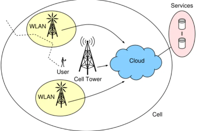
We consider the task assignment problem arising in the context of the mobile cloud computing (MCC). In MCC, the key idea is to offloadcomputationally demanding tasks to the cloud, process them there, and then transmit the results back to a mobile device [1], [2], [3] This can be faster and also consume less energy in the mobile device. The cloud could be accessed using the cellular network, or via a WLAN hotspot. The latter option is only intermittently available, but can offer significant advantages in terms of cost and energy [1]. The offloading scenario for a mobile user is illustrated in Fig. 1.
In MCC, three types of tasks can be identified: (i) those which can be processed only locally in a mobile device, (ii) those which are processed in the cloud, and (iii) those which can be processed either in the mobile or in the cloud. A first interesting question is when flexible type (iii) tasks should be processed locally and when in the cloud. Furthermore, for type (ii) and type (iii) tasks, there may exist multiple access links, with different characteristics (e.g., WLAN, LTE, 3G) to use for accessing the cloud. This leads to multi-dimensional considerations where, energy consumption, transmission costs, task type (e.g., background or foreground), network availabil-ity and rates, must be taken into account.
We approach this problem in the framework of Markov decision processes (MDP). The different options (process locally, or offload to a cloud, either at a hotspot or via a cellular network) are modelled as single server queues. The resulting dynamic decision problem is a specific type of a dispatching or task assignment problem, where the policy seeks to minimize a
given cost function (e.g., the mean response time). In contrast to the more common setting, in our case the servers corre-sponding to (WLAN) hotspots are available only intermittently due to the assumed mobility of a user. Moreover, some options can be expensive to use. For example, service time (but not the queueing delay) in a cellular connection can cost actual money, in particular, if the user is roaming abroad. Therefore, often well-functioning task assignment policies such as the join-the-shortest-queue (JSQ) and the least-work-left (LWL) may make sub-optimal decisions leading to poor performance. In contrast, the policies developed in this paper take into account the actual cost factors, the current state of the system (backlogs in different queues and the currently available networks), and the anticipated future tasks when making the decisions.
First we derive a new theoretical result, the so-called value function, for an M/G/1-queue with intermittently available server. The intermittently available server corresponds to the WLAN hotspots: tasks offloaded via WLAN may need to wait until the “server” appears again. Then, the value function derived for this particular type of M/G/1-queue, together with value functions for the other two options (local processing, offloading to the cloud through the cellular network), are used to apply the policy improvement step of the MDP framework. This yields a robust and efficient offloading policies that take into account the intermittent presence of WLAN hotspots.
Cloud Cell Services WLAN WLAN Cell Tower User
Fig. 1. Offloading in mobile cloud computing. The cloud services can be accessed via a cellular network or intermittently available WLAN hotspots.
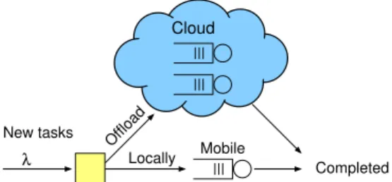
λ Offload New tasks Completed Locally Mobile Cloud
Fig. 2. Offloading in mobile cloud computing: some tasks can be processed either locally in a mobile device or in the cloud, where the latter involves also transmission costs in terms of energy, delay and money.
In addition to the offloading of computational tasks, mobile offloading is also seen as a promising candidate to deal with the rapidly increasing traffic volumes (see, e.g. [4], [5], [6]), as well as, for backup and synchronization traffic (e.g. Dropbox, Flicker, etc.) [7]. Typically the offloading mechanisms are heuristic and chosen with a particular scenario in mind. [8] proposes a simple model to study computation and transmis-sion energy tradeoffs, while [9] formulates an optimization problem involving various costs. Nevertheless, neither work considers queueing effects. Lee et al., in [6], develop a similar queueing model for the intermittently available server to ana-lyze the gain from offloading. However, no policy optimization is carried out.
The main contributions of this paper are as follows: 1) We analyze the offloading problem in MCC and propose
a multi-queue model to capture the essential elements. 2) We derive a new queueing theoretic result; the
size-aware value function for M/G/1-queue with an intermit-tently available server.
3) We give new state- and cost-aware offloading policies that take into account the mobility, the existing tasks, and the anticipated tasks. By means of numerical examples, we further demonstrate that significant gains can be available.
The rest of the paper is organized as follows. In Section II, we introduce the model and the notation. The value function for M/G/1 with intermittently available server is derived in Section III. Section IV describes the new dynamic offloading policies, which are evaluated in the numerical examples. Section V concludes the paper.
II. MODEL ANDNOTATION
Fig. 2 illustrates the basic setting, where three performance metrics are important to us: (i) energy consumption at the mobile device, (ii) monetary costs (from the access network), and (iii) the delay until the results are available for the user (i.e., the response time). Should a transfer of a content be carried out in the vicinity of WLAN hotspots, the transfer time can vary a lot depending on if an WLAN connection is currently available or not, whereas the use of a cellular connection is often slower and costs money. The cloud itself is assumed to be scalable and thus free from capacity concerns.
A. Task and Network Types
Different types of tasks emerge in a mobile device according to some process, which we, for simplicity, assume to be a Poisson process with rateλ. These tasks can be classified into the following three classes:
(i) Local-only:A fractionpmare unconditionally processed
locally in the mobile device, e.g. because transferring the relevant information would take more time and energy than when processed locally or because these tasks must access local components (e.g. sensors, user interface, etc.) [1]. Local processing consumes the CPU power of the device and, in particular, the battery power. We assume that jobs processed locally are served in the first-come-first-server(FCFS) order and for each task we know the expected service time (depends on the task and the CPU). There are no communication costs or delays. (ii) Cloud-only: A fractionpc must always be processed in
the cloud, e.g. because necessary data or the software is only present in the cloud. Backup or synchronization of files and images (e.g. Dropbox, Google+, etc.) could also be seen as such an “offloading task”. The user can still decide which network to use for offloading.
(iii) Flexible:Finally, a fractionp= 1−pm−pc are flexible
tasks that can be processed either in a mobile device or in the cloud. For these tasks, the device can dynamically decide where they are processed based on the urgency of the task, available networks and the state of the system (e.g., the current backlogs) in general. Many tasks fall in this category, and the offloading decision depends first on whether the communication costs balance the local processing costs [8].
All “cloud-only” tasks as well as some of the “flexible” ones, will need to access the cloud over some wireless interface. We assume the following options are available:
(a) Cellular network: When accessing the cloud via a cellular network, there is queueing due to the transmission speed of the cellular link. The service time consists of the upload time, cloud processing time, and the download time. For simplicity, we lump these three phases together and model them as a single FCFS server. Costs arise in terms of transmission delays (queueing and actual transmission times), energy and money costs related only to the transmission and reception (but not to processing). (b) WLAN: WLAN is similar to the cellular access with two distinctive features. First, the communication costs are generally lower (or even zero). Second, the hotspot availability is intermittent and the offloading may en-counter long random delays until the device arrives to a vicinity of the next hotspot. This intermittent availability of hotspots corresponds to a FCFS queue with a server that disappears occasionally. We assume that the sojourn time in a hotspot and the time to move from one hotspot to another are exponentially distributed with parameters
νA and νD. (The cellular connection and local CPU
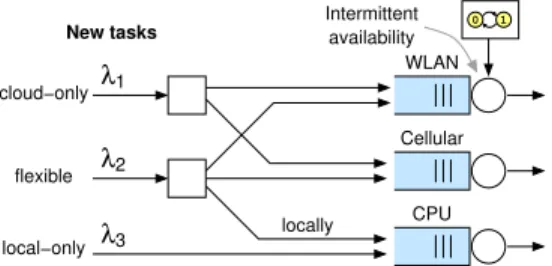
1 0 λ2 λ3 1 λ Intermittent availability CPU WLAN cloud−only flexible local−only New tasks locally Cellular
Fig. 3. Model: some tasks can be processed only in cloud, some locally and some are flexible.
B. Cost Structure and Objective
We take the users’ perspective and aim at maximizing his or her satisfaction. This involves energy consumption (unless the device is currently connected to a charger), monetary costs, and the delay. We further assume a time scale separation so that each task takes a short time when compared to a typical recharging cycle. The dynamic optimization problem is to strike a balance between the different costs factors and the perceived user experience in terms of delay (a.k.a., latency and response time). This boils down to two kinds of dynamic task assignment decisions as illustrated in Fig. 3: (i) choosing the cloud and the access link, or local processing for the flexible tasks, and (ii) choosing the cloud access link for the cloud-only tasks. The intermittent availability of the WLAN hotspots further complicates the problem.
We have different costs depending on what kind of actions a queue models (local CPU, or cloud via WLAN/cellular):
• Waiting costin queue while server is ON or OFF, which
is just a delay. No energy or money is spent while waiting, and this cost factor is also independent of the interface. The same holding cost applies also for the service time, as the user does not care where the delay occurs, just about the time it takes to complete a task.
• Energy cost, measured per bit, spent only when transmit-ting or receiving a task to/from a cloud. This cost depends on the interface. An energy cost is present also when a task is processed locally.
• Monetary cost, also measured per bit and spent only when transmitting or receiving a task to/from a cloud. This can be assumed to be zero for WLAN and some positive constant for the cellular access.
The complete model, illustrated in Fig. 3, is as follows:
• For each new task, the system must take anactionamong the available options (e.g., offload task ivia WLAN).
• Cost structure:
– Each taskjhas a task-specificholding costhj, which
characterizes its urgency (e.g., emails may have a lower priority than a response to the user activity).
– Cost parameters of Job j per each possible action i
are also known:
i) Energy consumption rate ej,i,
ii) Transmission cost rate cj,i, and
iii) Service timesj,i (excluding queueing delays).
• We are also aware of the full state, i.e., the files under transmission via different access links and the current state of the local processing queue, including the remain-ing service times of the jobs currently receivremain-ing service.
• The queues are assumed to operate independently at constant rate according to FCFS scheduling discipline.
• The objective is to minimize the costs the system incurs,
min n X j=1 (cj,d(j)+ej,d(j))Sj+hjTj ,
whered(j)is the decision for jobj,Sjis its service time
andTj the latency, i.e., the sum of the waiting timeWj
andSj,Tj=Wj+Sj.
Note that the unit holding cost, H = 1, corresponds to minimization of the mean latency. In general, with this cost structure each job, after the assignment, has a certain holding cost while waiting,hW, and another while receiving service, hS. We utilize this convention later in Section III-D. For
simplicity, we assume thatSj =sj,d(j), i.e., the actual service
time is known exactly for each possible action. Similarly, in the size-aware setting with FCFS, also the tentative waiting time
Wjis known exactly for each decision (later arriving tasks will
not cause any additional delays to the present tasks). That is, we know exactly the immediate cost of each action (waiting and service time of the new task), while the consequences on later arriving tasks have to be also taken into account.
III. ANALYSIS
In this section, we consider a single size-aware M/G/1-FCFS queue, where the (remaining) service times of the existing jobs are known. Our aim is to derive the value function, which characterizes the expected difference in costs a system initially in statezincurs when compared to a system initially in equilibrium. The single queue results are later utilized to evaluate the costs from assigning a new task to different queues in the offloading setting depicted in Fig. 3.
A. Value function and policy improvement
The notion of value functions is a fundamental element in solving MDP problems [10], [11], [12]. Formally, let Vz(t)
denote the costs a stochastic system incurs during time(0, t)
when the system is initially in some state denoted by z. Obviously, many systems incur costs at every time step and
limt→∞E[Vz(t)] = ∞. However, for ergodic systems the
expected difference in costs incurred between two initial states, z1 andz2, is finite,
lim
t→∞E[Vz1(t)−Vz2(t)]<∞.
Instead of choosing an arbitrary state (such asz2in above) as
a reference state, it is customary to compare the costs incurred from a given statezto the long-run average costs, leading to a formal definition of the value function (without discounting)
vz, lim
whererdenotes the (long-run) mean cost rate. Both the value function and the mean cost rate depend on the policy, vz = vz(α)andr=r(α).
The standard application of the value function is the policy improvement. Suppose that we have determined vz(α0)for a
basic policy α0. At some state, we have n possible actions
(e.g.,npossible ways to process a new task), having immedi-ate costsxiand resulting stateszi,i= 1, . . . , n. Thenactions
can be evaluated by xi+vzi, as =immediate z }| { (xi−xj) + =future z }| { (vzi−vzj),
clearly describes the relative expected cost of action i in comparison to action j. The policy improvement step defines a new policy αby choosing the action i∗ that minimizes the expected long-term costs,
i∗= argmin i
xi+vzi.
That is, for the current action one deviates from the basic policyα0, while the consecutive actions are according to it so
that vz(α0) can be utilized. The constant offset in the value
function is immaterial, and equally
argmin i
xi+ (vzi−v0),
where v0 denotes the value of an empty system. In policy
iteration, one repeats the same steps for the new policy α
iteratively until the policy converges and an optimal policy has been obtained.1 For more details on the value functions
and MDP in general, we refer to [10], [11], [12], and on the use in the task assignment setting, see e.g., [13], [14], [15], [16]. The general approach can be traced back to Norman [17]. B. M/G/1-FCFS with intermittently available server
The value function for the size-aware M/G/1-FCFS queue with an always available server has been derived in [15].
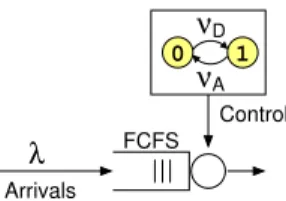
In this section, we consider the M/G/1-FCFS queue where the availability of the server is governed by an external ON/OFF process. In our context, the queue corresponding to offloading via WLAN is served only when the mobile device is in the vicinity of a WLAN hotspot, as illustrated in Fig. 1. More specifically, the server is either in ON-state processing the existing jobs in FCFS order (if any), or in OFF-state during which no job gets service. The server’s activity cycle is assumed to follow an external Markov ON/OFF process with independent activity and inactivity periods(Ai, Di), both
obeying exponential distributions with parametersνAandνD,
respectively. When a server returns, it resumes to serve the customer whose service was interrupted (if any), i.e., the work already conducted is not lost (cf. file transfers with resume).
The system is illustrated in Fig. 4. Hence, the fraction of time the server is available to process jobs is
P{available}= νD νA+νD
.
AsνD→ ∞, the availability of the server tends to1.
1To be exact, this holds, e.g., for ergodic systems with finite state-spaces, whereas with continuous state-space the situation is more complicated.
νA 0 1 νD Arrivals Control FCFS λ
Fig. 4. M/G/1-FCFS queue with an external ON/OFF process controlling the availability of the server.
1) Busy periods: A busy period begins when a job arrives to an empty system, and ends when the system becomes empty again. When a busy period ends, the server is obviously unconditionally active. Let q denote the probability that the server is active when a new busy period starts. Due to the memoryless property of the Markov processes, we have
q= λ λ+νA + νA λ+νA · νD λ+νD ·q, which gives q= λ+νD λ+νA+νD . (1)
The mean remaining busy period in a work-conserving M/G/1-queue is given by
u
1−ρ, (2)
whereuis the initial backlog andρ=λE[S]the offered load withE[S]denoting the mean service time. We can utilize (2) to give an expression for the mean busy period in a system with the intermittently available server as follows. First, we associate the interruptions occurring during the service time of Job ito be part of the corresponding job,
Yi=Xi+D (i)
1 +. . .+D (i) Ni,
whereNi∼Poisson(νAXi)andD (i)
j ∼Exp(νD). Thus, with
the chain rule of expectation one obtains
E[Y] = (1 +νA/νD) E[X], E[Y2] = (1 +νA/νD)2E[X2] + 2νA ν2 D E[X].
In this sense, the offered loadduringthe busy period is
ρ∗,λE[Y] =λE[X](1 +νA/νD).
For stability ρ∗ < 1 is assumed. The mean busy period can be obtained by utilizing (2), which gives the mean remaining busy period in an M/G/1-queue with an initial backlog ofu:
E[B] =q· E[Y] 1−ρ∗ + (1−q)· E[Y +D] 1−ρ∗ = E[Y] 1−ρ∗ + 1 1−ρ∗ · νA/νD λ+νA+νD = E[Y] +β 1−ρ∗ ,
where β denotes the mean time until the server becomes available at the start of the busy period,
β= νA/νD λ+νA+νD
2) Mean delay: The mean delay in an ordinary M/G/1-queue is given by the Pollaczek-Khinchine formula,
E[T] = λE[S 2]
2(1−ρ)+ E[S]. (3)
The following holds for the intermittently available server: Theorem 1: The mean delay in an M/G/1-queue with inter-mittently available server is given by
E[T] = λE[Y
2] 2(1−ρ∗)+
E[Y] +β(1 +λ(E[Y] + 1/νD))
1 +λβ . (4)
Proof: In an M/G/1-queue, where the first customer of a busy period receivesexceptional service, the mean delay is[18]
E[T] = λE[S
2]
2(1−ρ)+
2E[S∗] +λ(E[(S∗)2]−E[S2])
2(1 +λ(E[S∗]−E[S])) , (5)
where S∗ denotes the service time of the first customer, S
the service time of the other customers, and ρ=λE[S]. Our system is a special case of the above, where S=Y and
S∗=Y∗=
Y, with probability of q, Y +D, otherwise.
The first two moments of Y∗ are
E[Y∗] = E[Y] + νA/νD λ+νA+νD
= E[Y] +β, E[(Y∗)2] =qE[Y2] + (1−q) E[(Y +D)2]
= E[Y2] + 2 νA/νD λ+νA+νD E[Y] + 1 νD = E[Y2] + 2β E[Y] + 1 νD .
Substituting these into (5) gives (4).
Note that at the limit νD → ∞, we have β → 0 and (4)
reduces to the Pollaczek-Khinchine mean value formula (3). Another interesting limit is obtained when both νA, νD→ ∞
in such way thatνD/(νA+νA), corresponding to the fraction
of time the server is available, is finite (cf. duty cycle). C. Size-aware value function
As already mentioned, we assume a size-aware system, where the service times of the jobs become known upon arrival. We let∆idenote the (remaining) service time of Jobi,
which are ordered so that Job 1(if any) receives first service, then Job 2, etc. We also know the state of the server, i.e., whether it is available or not, but not how long each time period is going to last. The parameters of the availability process,(νA, νD), however, are known. The state of the system
is denoted by vector z,
z= (∆1, . . . ,∆n;e),
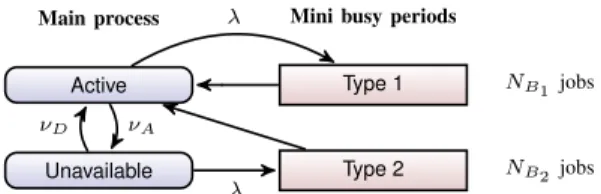
wheree∈ {0,1} indicates if the server is available or not. Our aim is to derive the size-aware value function with respect to delay (response time). To this end, we first recall that the mean number of jobs served during a busy period in an ordinary M/G/1-queue is [19] E[NB] = 1 1−ρ. (6) 00000000 00000000 00000000 00000000 00000000 00000000 00000000 00000000 00000000 11111111 11111111 11111111 11111111 11111111 11111111 11111111 11111111 11111111 000000000000 000000000000 000000000000 000000000000 000000000000 111111111111 111111111111 111111111111 111111111111 111111111111 Server unavailable
initially unavailable server Mini busy period w/
period ends when a mini busy Server always active
Time t
Time t
System 2
System 1
initially available server Mini busy period w/
D
X X
Initial time until server available
"Offset"
Mini busy period
Backlog u
Backlog u
Mini busy period
Fig. 5. Derivation of the value function by analyzing mini busy periods.
Utilizing the above, it is easy to show by conditioning that the mean number of jobs served during a busy period that starts with a job having a service time ofxis
E[NB|X1=x] = 1 + λx
1−ρ. (7)
Now we are ready to state our main theorem:
Theorem 2: The value function with respect to delay in an M/G/1-queue with intermittently available server is
vz−v0= λγ2u2 2(1−ρ∗)+ 1off λγu (1−ρ∗)ν D +γ n X i=1 (n+ 1−i)∆i+ 1off n νD , (8)
whereγ= 1 +νA/νD andρ∗=λ γE[X], and1off = 1if the
server is not currently available (e= 0) and zero otherwise. Proof: Fig. 5 illustrates a sample realization when the server is initially available, which happens with the probability ofq, see (1). The upper System 1 has an initial backlog ofu, and the lower System 2 is initially empty. The idea is that by assuming the same arrival sequences and server availabilities for both systems, we can deduce the mean difference in costs incurred until System 1 becomes empty, after which the two systems will behave identically. In what follows, we utilize the lack of memory property of Markov processes repeatedly without explicitly mentioning it.
Suppose a new job with size x arrives when the backlog in System 1 isu. This causes the backlog to jump fromuto
u+x. We refer to the time period until the backlog in System 1 is again at level uas amini busy period. During the other time periods, i.e., outside the mini busy periods, the “original” backlog is served and we refer to this asthe main process. First we observe that two types of mini busy periods can emerge: (i) those where the server is initially available (Type 1), and (ii) those where it is not (Type 2). Fig. 6 illustrates a high-level view on System 1. The two states on the left, active and unavailable, correspond to the main process, and the possible mini busy periods are on the right. We note that when a mini busy period ends, the server is always in active state.
Next we refer to Fig. 5, and observe that the durations of the mini busy periods and the new jobs involved are identical in both systems, and in fact a mini busy period in System 1 corresponds to a busy period in System 2. The only important difference is that the new jobs arriving during a (mini) busy period experience an additional delay in System 1 equal to the amount of backlog there was in System 1 at the beginning of the mini busy period (see the “offset” in Fig 5).
The number of Type 1 mini busy periods obeys Poisson process with mean λu. Associating the unavailability periods to the job currently under service, the remaining busy period is equivalent to one in an ordinary M/G/1-queue with service timeY. In particular, the mean number of jobs served during such a busy period is given by (6)
E[NB1] = 1 1−ρ∗.
The cost difference these jobs experience between the two systems is equal to the offset indicated in Fig. 5. These offsets are independently and uniformly distributed on (0, u) (cf. Poisson arrival process), i.e., the average additional delay in System 1 for each mini busy period is
γu 2,
where γ = 1 +νA/νD is the constant factor by which the
nominal mean service time E[X] is multiplied to include also the interruptions occurring during the service of the job,
E[Y] =γE[X]. Combining these gives the additional delay System 1 incurs in total on average during the Type 1 mini busy periods until System 1 becomes empty,
d1=λu· 1 1−ρ∗ ·γ u 2 = λγu2 2(1−ρ∗).
Consider next the time periods when the server in the “main process” is unavailable (i.e., excluding the mini busy periods, see Fig. 5). The key observation here is that these time periods end according to a Poisson process with rate λ+νD; either
a new job arrives and a mini busy period starts, or the server becomes available. In particular, at the end of Type 2 mini busy period the server is also available, and the unavailable time period has thereby ended, as illustrated in Fig. 6.
The number of times the server in the “main process” becomes unavailable obeys Poisson distribution with mean
νAu. With probability ofλ/(λ+νD)these time periods change
into the mini busy periods of Type 2. Thus, the mean number of Type 2 mini busy periods is
νAu· λ λ+νD
.
With Type 2 mini busy periods, we can associate the remaining time until the server becomes available to the job that started the mini busy period, corresponding to an effective service time of Y +D, where D ∼ Exp(νD). With aid of (7), it
follows that the mean number of jobs served during a Type 2 mini busy period is
E[NB2] = 1 + λE[Y +D] 1−ρ∗ = 1 +λ/νD 1−ρ∗ . Active Type 1 Unavailable Type 2 NB1jobs NB2jobs Main process λ Mini busy periods
νA .
λ νD
Fig. 6. State diagram illustrating how both Type 1 and Type 2 mini busy periods end with the server being available and active. The total time the main process spends in the “Active” state isu.
The mean additional delay in System 1 (the offsets) are statistically the same as earlier, γu/2, for each mini busy period. Thus the mean additional delay incurred during the Type 2 mini busy periods before System 1 becomes empty is again the product of the above: the mean number of Type 2 mini busy periods, times the mean number of jobs in each of them, times the average additional delay for jobs in System 1 in each mini busy period,
d2=νAu· λ λ+νD · 1 +λ/νD 1−ρ∗ ·γ u 2 = λγu2 2(1−ρ∗)νA/νD.
The average additional delay the later arriving jobs experience in System 1 is then
d1+d2=
λγ2u2
2(1−ρ∗), (9)
Additionally, we have the n jobs present only in System 1. The average delay they incur is
d3=γ(n∆1+(n−1)∆2+. . .+∆n) =γ n X
i=1
(n+1−i)∆i. (10)
Combining (9) and (10) gives the difference in the value function between state z and an empty system, vz−v0, for
the states where the server was initially available.
The case where the server is not initially available requires only two minor correction terms. If the server becomes available before a next job arrives, the remaining behavior is identical to what we just discussed with Type mini busy periods. However, with probability ofλ/(λ+νD), the initial
period when the server is unavailable ends to a specific (additional) Type 2 mini busy period. The offset for this mini busy period isu, since the server has been unavailable from the start. Thus the additional delay incurred in System 1 during this specific mini busy period is on average
λ λ+νD ·γu·1 +λ/νD 1−ρ∗ = λγu (1−ρ∗)ν D .
Similarly, the presentn jobs experience on average an addi-tional delay of n/νD before the server becomes available for
the first time, after which the situation is the same as with Type 1 and given by (10). Adding these two gives the additional mean delay incurred if the server is initially unavailable,
d4= 1off λγu (1−ρ∗)ν D + n νD .
We note that the terms with 1off factor correspond to the
additional penalty due to the currently unavailable server. Note also that the reference statev0corresponds to an empty system
with server initially in the same state as inz. This is sufficient for task assignment as inserting new jobs to a queue does not change the state of the server, the availability of which was governed by an external independent ON/OFF process. The parameter γ= 1 +νA/νD can be seen as the effective mean
service rate, asγucorresponds to the mean time to process a backlog of u(given the server is initially available).
The value function (8) is with respect to the delay. Next we will consider how much it costs to add a new job to a queue, i.e., we give an expression for the admission cost. We also generalize the cost structure to arbitrary and separate holding costs that apply for the waiting time and service time. D. Admission costs and general cost structure
Next we consider how much it costs in terms of additional delay all later arriving jobs concurrently incur if a job with size
x is admitted to the queue. The cost difference with respect to delay is simply the difference in the relative values,
a(x;z) =vz⊕x−vz, (11)
where z denotes the initial state and z⊕x the state after including a new job with sizex,
z⊕x= (∆1, . . . ,∆n, x;e).
Corollary 1: The admission cost of a job with size x
with respect to delay in an M/G/1-queue with intermittently available server is a(x;u) = λγx 1−ρ∗ γ(2u+x) 2 + 1off νD +γ(u+x) +1off νD . (12)
Proof: With FCFS, the admission cost depends only on the current backlog u= ∆1+. . .+∆n (later arrivals will not
delay the present jobs). Substituting (8) to (11) yields (12). Note thatγ→1andρ∗→ρwhenνD→ ∞, and the above
reduces to the admission cost in an ordinary M/G/1 [15],
a(x;u) = λx
2(1−ρ)(2u+x) +u+x.
The above value function is with respect to delay, corre-sponding to unit holding cost rate during both the waiting and service time. A generalization to arbitrary and separate holding cost rates for the waiting and service time is straightforward. This is important for us as itallows specifying energy, delay, and money costs per task once the assignment decision has been done and, e.g., the cost per bit transmitted gets fixed (recall that operators charge only for the bits transmitted).
Corollary 2: The admission cost of a job with sizexand holding cost rates (hW, hS)for the waiting and service time
to an M/G/1-queue with an intermittently available server is
a(x;u) = λE[HW]γx (1−ρ∗) γ(2u+x) 2 + 1off νD +hW γ(u+x)−x+1off νD +hSx. (13)
whereE[HW] is the mean waiting time holding cost rate for
jobs arriving to the queue.
Proof: First we note that the first two terms in (12) correspond to the additional delay the later arriving jobs experience on average if the new job is admitted to the queue. With non-preemptive scheduling disciplines, the service times of the jobs are not affected by the state of the system (at any moment), and thus the first two terms (12) must correspond to the increase in the waiting time, which we simply multiply by the mean holding cost while waiting, E[HW]. The costs the
given(x, hW, hS)-job incurs on average is
(u(1 +νA/νD) +x(νA/νD) + 1off/νD)hW +xhS.
Combining these yields (13).
The first term corresponds to the mean additional costs the later arriving jobs will incur (while waiting), and the last two terms to the costs the given new job incurs on average. The same generalization to job- and state-specific (waiting or in service) holding cost rates can be done also for the value function (8), which we omit here for brevity.
The obtained result (13) is satisfactory in many respect. First, the expression is compact and depends only on few parameters: the new task,(x, hW, hS), the state of the server
(available or not) and the current backlog u. The rest are constant, i.e., (13) is clearly easy to compute in online fashion. Second, (13) is insensitiveto the distribution of service time
X and depends only on its mean. Third, considering (13) as a conditional admission cost on condition that U = u, we note that the expected admission cost is also insensitive to the distribution of U and depends only on its mean E[U]. The insensitivity is a desirable property, e.g., towards the robustness and predictabilityof a control algorithm [20].
IV. DYNAMICMOBILEDATAOFFLOADING
In this section, we utilize the just derived value functions and admission costs to derive sophisticated dynamic policies for the offloading problem. The general approach is as follows: 1) We start with a static policy α0 (actions are made
independently of the past decisions and the state of the queues). Note that the actions ofα0may still depend on
the parameters of a task (e.g., size or holding costs). 2) Given a Poisson arrival process, the staticα0feeds each
server jobs also according to a Poisson process, the system of parallel queues decomposes, and the sum of queue specific value functions gives the value function for the whole system, vz=Piv
(i)
z(i).
3) Consequently, we can carry out the policy improvement step and simply choose for each task the queue with the smallest admission cost using (13),
α1: argmin
j
aj((x, hW, hS); (uj, ej)),
where (x, hW, hS)in general also depend on Queue j
(e.g., the service time depends on the link speed when offloading a task to a cloud), and (uj, ej) denote the
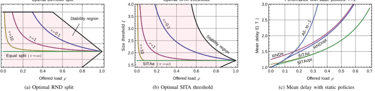
Stability region Ν=0.1 Ν=1 Ν= 10 Equal splitHΝ ® ¥L 0.0 0.2 0.4 0.6 0.8 1.0 0.4 0.6 0.8 1.0 Offered loadΡ Optimal split p
Optimal Bernoulli split
Ν= 0.1 Ν=1 Ν= 10 SITAe HΝ ® ¥L Stability region 0.0 0.2 0.4 0.6 0.8 1.0 1.5 2.0 2.5 3.0 3.5 4.0 Offered loadΡ Size threshold Ξ
Optimal SITA thresholds
All -to -1 RNDe RNDopt SITAe SITAopt 0.0 0.1 0.2 0.3 0.4 0.5 0.6 0.7 1.0 1.5 2.0 2.5 3.0 Offered loadΡ Mean delay E @ T D
Performance with static policies:Ν =1
(a) Optimal RND split (b) Optimal SITA threshold (c) Mean delay with static policies
Fig. 7. Example 1: Server 1 always available with service rater1= 1; Server 2 is intermittently available withνA=νD(i.e., 50%) andr2= 2.
We refer to the the improved policy as FPI (first-policy-iteration). The FPI policy is no longer static but dynamic, and in practice it is often also near optimal (given the starting point was a reasonable). Let us next first illustrate the concept and different heuristic policies with a toy example of two servers. A. Toy example
Consider first an elementary system of two queues:
• Server 1: always present; service rater1= 1
• Server 2: intermittently available, νA=νD=ν;r2= 2.
Hence, Server 2 is available50%of the time and the capacity of both queues is equal. With parameter ν we can adjust the length of the duty cycle. Job sizes are X ∼Exp(1).
The optimal Bernoulli (random) split between the two queues, determined using (4), is depicted in Fig. 7(a). Pa-rameter p on the y-axis corresponds to the fraction of jobs assigned to Server 1. For very small λ, it is advantageous to assign all jobs to Server 1 (p = 1). As λ increases, it first becomes advantageous and later necessary (ρ≥0.5) to utilize both servers (p <1). Whenν → ∞, the duty cycle in Server 2 becomes infinitely small and the two servers are equivalent. Consider next the size-interval-task-assignment (SITA) pol-icy, which assigns jobs shorter than threshold ξ to Server 1, and the rest to Server 2 [21], [22]. This way, the short jobs are segregated from the long ones and processed in the “faster” server (cf. SRPT). Hence, SITA controls both the load and the type of jobs each server receives. With SITAe, the threshold is chosen so that both servers receive equal load;ξe≈1.67835.
The optimal threshold for SITA can be determined using (4), and we refer to that policy as SITAopt. Fig. 7(b) depicts these for ν = 0.1,1,10. Observations are similar as with RND.
Fig. 7(c) depicts the mean delay with the different policies. All-to-1 means that all jobs are assigned to Server 1, and thus it is unstable whenρ≥0.5. We observe that the SITA policies are strong and the difference between them is negligible when
ρ >0.1in this case. In fact, SITA is the optimal static policy for ordinary FCFS servers with respect to delay [23].
Let us then consider the following dynamic policies:
• JSQ chooses the queue with the least number of jobs. • LWL chooses the queue with the shortest backlog. • Greedy is the same as LWL, but includes the availability.
• FPI based on the SITAe.
RNDopt SITAopt JSQ LWL Greedy FPI 0.0 0.2 0.4 0.6 0.8 0.8 0.9 1.0 1.1 1.2 1.3 Offered loadΡ E @ T D E @ TGreedy D
Performance with dynamic policies:Ν=1
Fig. 8. Relative mean delay with dynamic policies. FPI outperforms all other policies even in this very elementary setting.
In each case, possible ties are broken in favor of Server 1. The numerical results are depicted in Fig. 8. On the x-axis is the offered loadρ, and they-axis corresponds to the mean delay relative to the mean delay with Greedy. FPI, the only policy thatconsciouslytakes into account also the anticipated future arrivals shows superior performance whenρ→1.
B. Mobile data offloading example
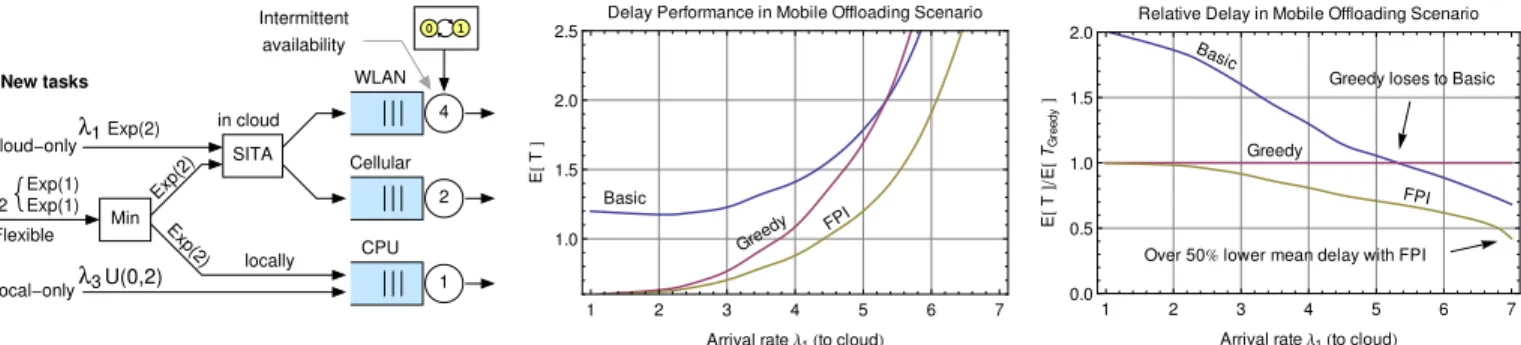
Let us finally consider the task offloading scenario depicted in Fig. 9 (left). The chosen parameters facilitate analysis.2 The always offloaded tasks X1 arrive at rate λ1 where X1 ∼ Exp(2). Flexible jobs (X2,C, X2,L) arrive at rate λ2, where X2,C denotes the size if offloaded, and X2,L if
processed locally. We assume that X2,C and X2,L are i.i.d., X2,C ∼X2,L∼Exp(1). Jobs that the local CPU must process
arrive at rateλ3 and are uniformly distributed,X3∼U(0,1).
Then νA = νB = 0.25 and the objective is to minimize the
mean delay. We consider the following policies:
• Basicpolicy comprises two heuristic decisions. First, the flexible jobs are processed locally if X2,C > X2,L, and
otherwise offloaded to the cloud. Offloaded tasks are split with SITAe: short jobs are transmitted via a cellular network, and long ones via WLAN hotspots.
• Greedy policy chooses the action which minimizes the expected delay of the given task. The current system state and tentative service times are utilized in myopic fashion. 2Note that the approach itself is general. These examples are chosen partly due to the analytical tractability, and partly due to the limited space.
1 0 Exp(2) Exp(2) Exp(2) New tasks locally in cloud U(0,2) Min SITA CPU Cellular WLAN Intermittent availability 1 2 4 λ3 2 λ λ1 Flexible Exp(1) Exp(1) Local−only Cloud−only Basic Gree dy FPI 1 2 3 4 5 6 7 1.0 1.5 2.0 2.5
Arrival rateΛ1Hto cloudL
E
@
T
D
Delay Performance in Mobile Offloading Scenario
Basic
Greedy
FPI
Greedy loses to Basic
Over 50%lower mean delay with FPI
1 2 3 4 5 6 7 0.0 0.5 1.0 1.5 2.0
Arrival rateΛ1Hto cloudL
E @ T D E @ TG re e d y D
Relative Delay in Mobile Offloading Scenario
Fig. 9. Example 2: Dynamic offloading scenario. WLAN is available50%of the time (νA=νD= 1/4) and has service rater1= 4. Cellular has service rater2= 2and the CPU is the “slowest” withr3= 1. The mean delay is depicted for fixedλ2=λ3= 1. FPI achieves the clearly lowest mean delay.
• FPI policy is obtained by computing the parameters of
the arrival process to each queue with the above basic policy, and then using (12) to evaluate each action. As Basic is a static policy, its mean delay performance can be computed analytically using the Pollaczek-Khinchine mean value formula and (4). The other two must be evaluated by means of simulations. In our test scenario, we set λ2=λ3=1,
and vary λ1. In this case, Basic is stable for λ1<7.5.
Fig. 9 (middle) depicts the mean delay as a function of
λ1, and Fig. 9 (right) the relative mean delay when compared
against the Greedy policy. Initially, both Greedy and FPI offer a low mean delay, as expected. However, as the load increases, Greedy starts to suffer from its short-sighted decisions, and eventually it falls even behind Basic. In contrast, FPI shows again superior performance and outperforms the other two especially when the load is high, where the mean delay with Greedy is more than two times higher than with FPI.
V. CONCLUSIONS ANDFUTUREWORK
In this paper, we have developed a stochastic model to study the dynamic offloading in the context of MCC. The model captures various performance metrics and also intermittently available access links (WLAN hotspots). The problem itself is far from trivial, and to facilitate analysis, we have, e.g., assumed that a job set to be offloaded via WLAN hotspot cannot be later re-assigned to cellular, known as jockeying in the queueing literature. The analysis is carried out in the MDP framework. First we derived a new queueing theoretic result, which enables derivation of near-optimal dynamic offloading policies that take into account the various performance metrics (delay, energy, offloading costs), current state of the queues, and the anticipated future tasks. In the preliminary numerical experiments, the resulting policy gave very good results and outperformed other policies by a significant margin. The gain is expected to be even higher with more diverse cost structures. The future work includes experiments in more realistic scenarios, where, e.g., energy consumption and transmission costs of cellular data plan are explicitly included. Moreover, we plan to investigate the possibility to develop schemes with jockeying, where it is possible to re-assign tasks later on. This can be extremely useful, e.g., if a user unexpectedly arrives to the vicinity of a hotspot.
REFERENCES
[1] E. Cuervo, A. Balasubramanian, D.-k. Cho, A. Wolman, S. Saroiu, R. Chandra, and P. Bahl, “Maui: making smartphones last longer with code offload,” inProc. of ACM MobiSys, 2010.
[2] B.-G. Chun, S. Ihm, P. Maniatis, M. Naik, and A. Patti, “Clonecloud: elastic execution between mobile device and cloud,” inProc. of EuroSys ’11, 2011.
[3] S. Kosta, A. Aucinas, P. Hui, R. Mortier, and X. Zhang, “Thinkair: Dynamic resource allocation and parallel execution in the cloud for mobile code offloading,” inProc. of IEEE INFOCOM, 2012. [4] A. J. Nicholson and B. D. Noble, “Breadcrumbs: forecasting mobile
connectivity,” inACM MobiCom’08, 2008, pp. 46–57.
[5] A. Balasubramanian, R. Mahajan, and A. Venkataramani, “Augmenting mobile 3G using WiFi,” inACM MobiSys’10, 2010, pp. 209–222. [6] K. Lee, J. Lee, Y. Yi, I. Rhee, and S. Chong, “Mobile data offloading:
How much can wifi deliver?”IEEE/ACM Transactions on Networking, vol. 21, no. 2, pp. 536–550, 2013.
[7] M. V. Barbera, S. Kosta, A. Mei, and J. Stefa, “To offload or not to offload? the bandwidth and energy costs of mobile cloud computing,” inProc. of IEEE INFOCOM, 2013.
[8] K. Kumar and Y.-H. Lu, “Cloud computing for mobile users: Can offloading computation save energy?”Computer, vol. 43, no. 4, 2010. [9] Y. Im, C. J. Wong, S. Ha, S. Sen, T. Kwon, and M. Chiang, “AMUSE:
Empowering users for cost-aware offloading with throughput-delay tradeoffs,” inProc. of IEEE Infocom Mini-conference, 2013.
[10] R. Bellman,Dynamic programming. Princeton University Press, 1957. [11] R. A. Howard,Dynamic Probabilistic Systems, Volume II: Semi-Markov
and Decision Processes. Wiley Interscience, 1971.
[12] M. L. Puterman,Markov Decision Processes: Discrete Stochastic Dy-namic Programming. Wiley, 2005.
[13] K. R. Krishnan, “Joining the right queue: a state-dependent decision rule,”IEEE Transactions on Automatic Control, vol. 35, no. 1, 1990. [14] ——, “Markov decision algorithms for dynamic routing,”IEEE
Com-munications Magazine, pp. 66–69, Oct. 1990.
[15] E. Hyyti¨a, A. Penttinen, and S. Aalto, “Size- and state-aware dispatching problem with queue-specific job sizes,” European Journal of Opera-tional Research, vol. 217, no. 2, pp. 357–370, Mar. 2012.
[16] E. Hyyti¨a, S. Aalto, and A. Penttinen, “Minimizing slowdown in heterogeneous size-aware dispatching systems,” ACM SIGMETRICS Performance Evaluation Review, vol. 40, pp. 29–40, Jun. 2012. [17] J. M. Norman,Heuristic procedures in dynamic programming.
Manch-ester University Press, 1972.
[18] D. Gross, J. F. Shortle, J. M. Thompson, and C. M. Harris,Fundamentals of Queueing Theory, 4th ed. John Wiley & Sons, 2008.
[19] L. Kleinrock,Queueing Systems, Volume I: Theory. Wiley, 1975. [20] T. Bonald and A. Prouti`ere, “Insensitivity in processor-sharing
net-works,”Perform. Eval., vol. 49, no. 1-4, pp. 193–209, Sep. 2002. [21] M. E. Crovella, M. Harchol-Balter, and C. D. Murta, “Task assignment
in a distributed system: Improving performance by unbalancing load,” in
SIGMETRICS’98, Madison, Wisconsin, USA, Jun. 1998, pp. 268–269. [22] M. Harchol-Balter, Performance Modeling and Design of Computer Systems: Queueing Theory in Action. Cambridge University Press, 2013.
[23] H. Feng, V. Misra, and D. Rubenstein, “Optimal state-free, size-aware dispatching for heterogeneous M/G/-type systems,”Performance Eval-uation, vol. 62, no. 1-4, pp. 475–492, 2005.