R - Statistical and Graphical Software Notes

R

- Statistical and Graphical Software Notes

School of Mathematics, Statistics and Computer Science

University of New England

• R Murison,[email protected]

R

programming guide

Printed at the University of New England, December 12, 2005

Contents

1 Introduction 1

1.1 Why useR? . . . 1

1.2 Scope of these notes . . . 2

1.3 History ofR . . . 3

1.4 R Resources . . . 4

1.5 The purpose of the examples . . . 5

1.6

Expertise through practice

2

R

in the Windows Operating System

2.2 A test run withR in Windows . . . 7

2.3 Help . . . 12

3 R in the Linux Operating System 13 3.1 Installation . . . 13

3.2 A test run – Linux . . . 13

3.3 Help . . . 15 4 Examples(1) 17 5 Elements of R programs 18 5.1 Input . . . 18 5.2 Processing . . . 19 5.3 Output . . . 19 5.3.1 Saving text . . . 19 5.3.2 Saving Graphs . . . 20

5.4 Multiple Graphics windows . . . 21 6 Troubleshooting: FAQ

by Ms J Reid

Chapter 1

Introduction

1.1

Why use

R

?

As a scientist, you will collect experiment data and analyse them as part of the scientific method. In all but trivial experiments, the data are complex and understanding the in-formation in them is done using graphics and statistical models. Graphics and modelling are done with a computer program and computing is just one of the skills necessary for a scientist. Training in the R statistics and graphics package provides this skill.

Early exercises in your statistics units may not be complex as they are the building blocks for further statistics and so it may even appear an overkill to use R when the calculations could be achieved simpler. But the objective is to learn statistics in order to be a competent scientist who can at least engage with a statistician and part of that training involves statistical computing. Thus although we start with simple problems which could be done as easily by other ways, we require that these problems be done inR to gain the expertise necessary for real-life problems where the complexity exceeds the capabilities of simplistic software.

The following list is also support for R .

• It is free, see [2], and because leading developers of statistical software are writing functions for this package. Thus competency in R means you can stay up to date with statistics.

• It covers statistical applications from the simplest to the complex and would allow you to complete all your statistical training usingR. Also, it treats different topics in a consistent way so that the programming you learn for say linear models will also be done the same way for non-linear models. This consistency is convenient but also gives an understanding of statistical modelling.

• Rhas a powerful suite of functions that allow you to use modern statistical methods. Modern statistics has simplified many problems through the use of graphics and computer intensive ideas.

2 CHAPTER 1. INTRODUCTION

• It involves the biggest concentration of statisticians worldwide so you have access to the best and most efficient methods. You will certainly encounter R beyond UNE. • The apparent simplicity of software such as MINITAB is superficial as it is limited

in the analyses that it can handle.

1.2

Scope of these notes

We assume that readers are familiar with the fundamentals of a computer such as is taught in primary and secondary schools and that they are also familiar with the computer they are using. You make seek help from us on statistical computing but would need to source help elsewhere for the basics of computing.

These notes are a guide for getting started with R . The intention is to help you to the stage where you can recognise the fundamentals of the program in order to follow the examples and exercises in the statistics units you encounter.

It is not intended that these notes be a compehensive manual for R . The computing of models is fundamental to statistics but the computing is learnt in conjunction with the statistics. These notes merely augment the unit notes in statistics.

At first glance, the volume of new material may appear daunting. The way to learn computing is to practise. Errors are to be expected but they provide the feedback which leads to better understanding. If you try each idea, one-at-a-time, the big picture will soon emerge and increasing familiarity will simplify the tasks.

For many, it will only be necessary to cover chapters 1, 2 or 3, 4 at first. The other chapters might be useful adjuncts when you encounter exercises in your statistics units.

The examples given in this guide do not necessarily relate to the statistics unit you are studying. The examples have been chosen to demonstrate the R computing. If the statis-tical reasoning is not initially apparent in these exercises, we recommend that you proceed by typing the commands as given, and when you have generated output the statistical parts may be clearer.

You may have to let go some of the obsolete notions with which you are comfortable in order to make progress in modern statistical and computing thinking. We draw your attention to ”Attributes of a UNE Graduate”

(http://www.une.edu.au/offsect/une grad attributes.htm)

where Communication Skills, Information Literacy, Problem Solving and Social Respon-sibility are goals for us all. You will be offered opportunities to enhance these traits in gaining expertise with R .

The R code for the examples can be obtained from the link at:-http://mcs.une.edu.au/∼Rguide

and if you download these, you can compute along with this guide in a self help tutorial. Chapter 2 gives directions for installing the program and a test run to ensure all is working using the Windows operating system. The linux counterpart of this is in Chapter

1.3. HISTORY OF R 3 3. Chapter 4 contains another simple example as training.

This is followed in Chapter 5 by a guide to the wayRworks using functions and assigning the results to an object. The program is more advanced than menu-based software which cannot handle modern statistical modelling. The way to source scripts from a file and to sink output to a file are explained in this chapter.

The important functions for reading and writing data are presented in Chapter 6. Chapter 7 discusses the objects in anRprogram, data frames, variables etc and Chapter 8 discusses how R organises its functions and objects.

Chapter 9 discusses different data types (with examples), Chapter 10 shows how to extract components of objects and Chapter 11 uses examples to illustrate the basics of plotting data.

The citation for R is given at [1], resources are located at [2] and you can link with r-help at [3].

1.3

History of

R

In the mid 1980’s, statistical software named S was developed at AT&T in New Jersey using the interpretative computer language Scheme. It was written to handle statistical modelling and designed to be extendable without modifications. Although it has expanded manyfold with extra functions and capabilities, it remans in the same form after 2 decades.

S morphed into S-PLUS and became a commercial package. In 1994, Ross Ihaka and Robert Gentleman at Auckland University wrote the first version of an S like software package and named it R , continuing in the Computer Science tradition eg C, S. They made their software freely available and this gesture captured the spirit of other software developers (Luke Tierney had developed Lisp-Stat, Martin Maechler had written Emacs Speaks Statistics) whence they joined forces. R continues to grow and is now supported by leading statisticians and computer scientists world-wide. It is open source software and is available freely

Whilst R appears similar to S or S-PLUS, it is different. Nevertheless, the book by Venables and Ripley ([4]) is an excellent reference and Dalgaard’s book ([5]) is a specialist introduction to R . The web site [2] has other detailed guides that have more depth than these notes.

4 CHAPTER 1. INTRODUCTION

1.4

R

Resources

There are versions for Linux, Mac and Microsoft. You find these at

either:-(i) the mirror site at UNE, http://mcs.une.edu.au/CRAN/ or

(ii) a CD distributed by the School of Mathematics, Statistics and Computer Science at UNE. The CD contains all the software used in the school including LaTeX, SciLab, Ghostview, Emacs.

It sometimes takes about 1 hour of internet time to download at home, about 5 minutes to install.

1.5. THE PURPOSE OF THE EXAMPLES 5

1.5

The purpose of the examples

Examples demonstrate the use of R to compute and then plot results. They are not necessarily related to the part of the unit you are studying; their purpose is to teach the basics of R .

Explanation of example 2.1/3.1

Random numbers (akin to a Lotto draw) are generated and the pattern of the frequency of these random numbers follows the familiar normal or bell-shaped distribution. Do not concern too much at the statistics but enter the code as listed and run the program. If you successfully run the program you have achieved the objective.

The normal distribution is characterised by its location (the mean) and spread (the standard deviation). The diagram in Figure 1.1 shows how its curve is derived from these 2 numbers. This is a general representation and in the values in the first exercise (chapter 2 for Windows and chapter 3 for Linux), are mean (= 2) and standard deviation (= 3).

Figure 1.1: Curve of the normal distribution

x mean - 3 sd mean - sd mean + sd mean + 3 sd

mean

inflection point inflection point

1.6

Expertise through practice

It is important that you gain competence with practice. You will soon pick up the style of R, realise that there is a way to get the appropriate answer and home in on that method. The following suggestions will assist in removing complexity about R.

• Consider the examples

• Try the functions on simple exercises and examine the results • Use the HELP files

Chapter 2

R

in the Windows Operating System

Denote 2 areas on theC: drive of your computer, 1. Where you save the R install program: C:\RHOME

2. Where you save your program files for analysing data: C:\Rwork

2.1

Installation

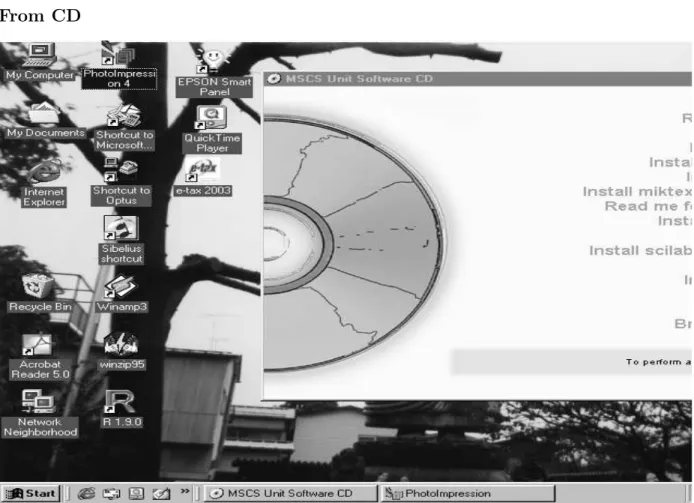
From CD

1. Insert the CD and select Install R from the menu box. (see Figure 2.1). Use the Install wizard to build R .

2. Upon completion, a blue R icon will appear on the desktop.

3. Also install Ghostscript and GSview as these programs are used for saving plots.

Figure 2.1: Installing from the Maths/Stats disk

2.2. A TEST RUN WITH R IN WINDOWS 7 From internet, CRAN website & Ghostscript

1. Use your internet browser ( eg Internet Explorer, Netscape or Mozilla) to point to : http://mirror.aarnet.edu.au/pub/CRAN or

http://mcs.une.edu.au/CRAN/ (see Figure??).

Under the heading Precompiled Binary Distributions, choose the link Windows. Next heading is R for Windows; choose the link base.

2. Next choose rw2.2.0-win32.exe1.

Save this to the folder C:\RHOME on your PC.

When downloading is complete, close or minimize the internet browser. 3. Double click on rw2.2.0-win32.exein C:\RHOME to install.

4. Install Ghostscript and GSview. The .exe files are obtained from:-http://www.cs.wisc.edu/∼ghost/

These programs are useful for graphics files.

2.2

A test run with

R

in Windows

Purely interactive

Double click the R icon on the Desktop and the R Console will open. Wait while the program loads. You observe something like this:

8 CHAPTER 2.

R

IN THE WINDOWS OPERATING SYSTEM

At the R prompt (>) (in the R console window), type :

x <- 1:20

plot(x,log(x),type=\’b\’)

The assignment operator ( <- ) is 2 keystrokes; < followed by - .

Now x contains the numbers 1,2,3,...,20 and the plot command produces a graph of log(x) vs x in the graphics window showing the individual points connected by lines.

Try typing plot(x,log(x),type=’l’) where the plot type is a line plot.

This is indicated by the letter ell, not the numeral 1. These are difficult to distinguish so care is necessary.

Executing an

R

command file

Your statistical computing requirements will rapidly outstrip the one–line interactive com-mands and so ascript fileof commands will need to be created via an editor. The program then executes the commands from the script file.

The script editor

TheFile menu in the toolbar of theR console has an item calledNew script. This opens an editor for entering a sequence of commands. Type the commands into the script window.

2.2. A TEST RUN WITH R IN WINDOWS 9 Ensure that you save the script by either

• Ctrl S

• From the toolbar choose File ⇒Save As

At this point notice that the foreground (or active) window has a blue border and the background window has a grey border. The functions on the toolbar will refer to the active window.

Example 2.1

In the following examples, we will use R to produce 100 Normally distributed random numbers with a mean of about 2 and a standard deviation of roughly 3. In each section, the different ways of producing this output will be demonstrated. A fuller description of this exercise is provided in Chapter 1 on page 5.

Enter the commands in the script window and save the file as rnorm.R, in C:\Rwork.

nrv <- rnorm(mean=2,sd=3,n=100)) print(summary(nrv) )

hist(nrv)

You are now ready to process the commands contained in the file rnorm.R using R . • Choose File in the toolbar of the R console window.

• In the dropdown menu, choose Change dir. . . , and choose the directory containing rnorm.R by browsing your file system, eg, C:\Rwork

This is often forgotten and the source of unnecessary help requests.

•ChooseFile, then chooseSourceRcode. . . from the dropdown menu. Finally highlight the file rnorm.R in the Folder window.

10 CHAPTER 2.

R

IN THE WINDOWS OPERATING SYSTEM

R then executes the commands contained in the file rnorm.R. It displays (a) a statistical summary of these numbers,

(b) a histogram of frequencies in the Graph window. These are the operations that have been calculated:-• nrv <- rnorm(mean=2,sd=3,n=100)

The R function rnorm produces Normally distributed random numbers and these numbers are assigned to anobjectcallednrv. The arguments are the mean, standard deviation and the sample size (n). For information on this function in R , type help(rnorm) in the R console.

• summary(normal.rv)

will give you a summary of 100 normal numbers, eg, mean = 1.8 (or similar), etc • hist(nrv)

will produce a histogram of the 100 random numbers in the R graphical window. To see the full output, you may have to edit theRgenerated command (in theRconsole)

source("C:/Rwork/rnorm.R") to

source("C:/Rwork/rnorm.R",echo=T)

This can be effected by use of the ↑ key, and insertion of the string echo=T followed by resubmission of the changed command. The other keys ←, → and ↓ perform the corresponding expected functions.

2.2. A TEST RUN WITH R IN WINDOWS 11

Tinn-R

An editor designed to be used with R in Windows is Tinn-R which may be downloaded from

http://www.sciviews.org/Tinn-R/ It self installs with a double click.

This is an alternative to the script editor that is built in the R console. Some people may prefer its facilities but if you are content with the script editor, you may elect to not worry about Tinn.

Once installed, R files are associated with There is a this editor and double clicking on the file icon will open it in Tinn. The editor colour codes objects, quoted text and indicates matching brackets when typing the script. The toolbar has functions for sending the script to the R program either the whole script or a selection. This is useful when debugging a program to locate exactly where the errors occur.

You use it in this

way:-1. Start R by double clicking the blue R icon on the desktop.

2. Change to the working directory , i.e. where the script file is saved.

3. Double click (Left Mouse Button) on the file icon, rnorm.Rto open in Tinn. 4. Find R on the Tinn toolbar.

5. From the drop down menu, choose Send File to R or 6. Send selection to R if you are testing part of your code.

12 CHAPTER 2.

R

IN THE WINDOWS OPERATING SYSTEM

Modifying an

R

command file

Use an editor (e.g. Tinn-R) to change the filernorm2.Rso that 1000 points are generated instead of 100. Then execute the new version of the file in R to produce the results for 1000 points.

Quitting

After inspection, quit the R program by typing, q()

and before the program closes down, you will be asked Save workspace image? [y/n/c]:

respond with y. This will be explained later.

2.3

Help

The program comes with comprehensive documentation on each function. You may ponder about some of the functions, egmean() or boxplot().

Windows help files

rw2000.exebuilds the Help pages. Use Helpin the toolbar.

Interactive

You can examine what you have done interactively by just typing the object, eg x <- 1:20 # make a list 1,2,3,4, ... ,20

x # check it

v <- seq(2,50,2) # make a list 2,4,6,8, ... ,50

v # check it

( The# symbol indicates a comment and the code between # and the end of the line is not processed.)

The help() function can be invoked interactively as in help(mean) or

Chapter 3

R

in the Linux Operating System

Locate the program source at (a) theCRANweb site, (b) theturing web site or (c) the CD.

3.1

Installation

Make a directory on your computer to store the program, eg. /usr/lib/R

If say you are a Linux Redhat user, the links are Linux →redhat→ 9.x/ → i386/ . Do similarly for Mandrake, Debian or suse.

Download R-1.9.1-0.fdr.4.rh90.i386.rpm 1 to the directory /usr/lib/R . Build the program

by:-1. login as su

2. type rpm -hUv R-1.9.1-0.fdr.4.rh90.i386.rpm

3.2

A test run – Linux

Purely interactive

Move to an appropriate directory, say ~\Rwork . Type : R and at the R prompt (>) type :

x <- 1:20

plot(x,log(x),type=’b’)

The assignment operator ( <- ) is 2 keystrokes; < followed by - .

The objectxcontains the numbers 1,2,3,...,20 and theplotcommand produces a graph of log(x) vs x in the graphics window.

1_{The version number may change with new releases, eg,R-2.0.0-0.fdr.4.rh90.i386.rpm .}

14 CHAPTER 3. R IN THE LINUX OPERATING SYSTEM

Try typingplot(x,log(x),type=’l’) where the plot type is a line plot. This is indicated by the letterell, not the numeral 1. These are difficult to distinguish so care is necessary.

Executing an

R

command file

Your statistical computing requirements will rapidly outstrip the one–line interactive com-mands, and so a file of commands will need to be created via an editor.

In the following examples, we will use R to produce 100 Normally distributed random numbers with a mean of about 2 and a standard deviation of roughly 3. In each section, the different ways of producing this output will be demonstrated. A fuller description of this exercise is provided in Chapter 1 on page 5.

Example 3.1

Using your favourite editor (eg Emacs, VIM, Kwrite) create a file calledrnorm.rcontaining the following commands :

normal.rv <- rnorm(mean=2,sd=3,n=100) print(summary(normal.rv) )

print(hist(normal.rv))

To execute this file of commands in file rnorm.r inR : 1. Move to the directory containing rnorm.r

2. Type R

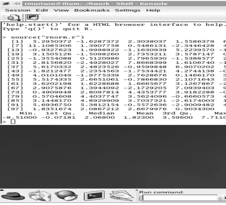
3. At the R prompt (>) type source("rnorm.r")

R then executes the commands contained in the filernorm.r. The program generates random numbers and plots a histogram.

A screen-capture of the file, the R console and the X11() graphics window is shown in Figure 3.1.

These are the operations that have been calculated:-• normal.rv <- rnorm(mean=2,sd=3,n=100)

TheRfunctionrnormproduces Normally distributed random numbers and assigns it to the object normal.rv. The arguments are the mean, standard deviation and the sample size (n). For information on this function inR , type help(rnorm) in theR

console.

• summary(normal.rv)

will give you a summary of 100 normal numbers, eg, mean = 1.8 (or similar), etc • hist(normal.rv)

will produce a histogram of the 100 random numbers in the R graphical window. To see the full output, you may have to change the R generated command

source("rnorm.r") to source("rnorm.r",echo=T).

3.3. HELP 15

Modifying an

R

command file

Use an editor to change the file rnorm2.r so that 1000 points are generated instead of 100. Then execute the new version of the file in R to produce the results for 1000 points.

Quitting

After inspection, quit the R program by typing,

q()

and before the program closes down, you will be asked

Save workspace image? [y/n/c]:

respond with y. This will be explained later.

3.3

Help

The program comes with comprehensive documentation on each function. You may ponder about some of the functions, egmean() or boxplot(). After starting R , enter

> help.start()

This will set up the help files in a html document; bookmark it straightaway.

Interactive

You can examine what you have done interactively by just typing the object, eg

x <- 1:20 # make a list 1,2,3,4, ... ,20

x # check it

v <- seq(2,50,2) # make a list 2,4,6,8, ... ,50

v # check it

( The# symbol indicates a comment and the code between # and the end of the line is not processed.)

The help() function can be invoked interactively as in help(mean) or

16 CHAPTER 3. R IN THE LINUX OPERATING SYSTEM

Chapter 4

Examples(1)

Example 4.1

This exercise is taken from Dalgaard (2002). Follow the procedures documented in Example 1.

1. enter these commands into a file, named bwi.R.

weight <- c(60, 72, 57, 90, 95, 72)

height <- c(1.75, 1.80, 1.65, 1.90, 1.74, 1.91) bmi <- weight/height^2

plot(weight ~ height)

2. In the R console, either

(a) Linux or Windows or Mac:- type source("bwi.R") or,

(b) Windows:- Use the Source R code. . . from the dropdown Files menu. 3. at the >prompt, type bmito see the calculated numbers.

This example uses data provided by the user instead of the numbers generated by the program in Example 2.1/3.1.

Data are usually read from a file rather than entering the numbers in a program.

Chapter 5

Elements of R programs

As in all programming we require

• Input - get the functions into the program, • Process the script to produce output • Save the output

The test job, rnorm.r, serves to identify the components and is listed here again for convenience.

normal.rv <- rnorm(mean=2,sd=3,n=100) print(hist(normal.rv))

5.1

Input

This has already been encountered with the test run that produced a histogram.

The source() function instructs the R program to accept the commands from a file. The file name, enclosed in quotes, is given as the argument, eg source("rnorm.r") .

The commands could be entered interactively by typing them singly into the R console but the inefficiency of this is obvious. A file such as rnorm.r can be kept for editing and is a reminder of what was done.

The choice of name for the file is arbitrary but the convention of using the .r suffix is useful, especially for Windows users. It is also useful to label the file with an informative name so that it may be recalled later. File names such asjob.r,prog.r,test.r,stats.r are vague and as likely their contents not easily recalled.

5.2. PROCESSING 19

5.2

Processing

There are 3 elements in the processing, (i) A function processes the information

(ii) The results of that function are assigned to an object.

(iii) The object is saved and can be printed or used in further calculations.

In a sense, the object is akin to a memory location on a calculator. The assignment operator has been mentioned previously; it is <- . The functionmustbe associated with brackets and the contents of the brackets are the arguments which will be processed by the function.

The lines of code inrnorm.rserve as examples to indicate specifically how the program is functioning.

In the first line, interpret the computation right to left. Thernorm()function generates random numbers from a normal distribution and the arguments are used in the calculations, n being the sample size. The results of this calculation are assigned to an object called normal.rv so that they they are “stored” and can be used later.

The choice of object names is arbitrary, instead of normal.rv, the object may have been calledz or any other name. In large jobs it pays to use informative, but not verbose, names for the objects. Conversely, the name of the function, rnorm(), has to be exact. Names of functions are case specific.

At this point, we do not observe any output as the results ofrnorm()have been directed to an object. The next line does not direct the output to an object so the output goes to the default which is the graph window in this case.

The line

print(hist(normal.rv))

evaluates 2 functions; the results from hist() are passed to the print() function. The manner is obvious - the innermost function is evaluated first and its results become the argument for the next, outermost function.

5.3

Output

The default outputs are the console for text and the graphics window for graphs.

5.3.1

Saving text

To get output on the screen, one would type:-print(normal.rv)

20 CHAPTER 5. ELEMENTS OF R PROGRAMS

To redirect the output to a file for later use, the sink() function works similar to the source() function, eg

sink("normRV.txt") print(normal.rv) sink()

The command, sink("normRV.txt") indicates that subsequent output will be saved in the file named normRV.txt. The direction to that file ends when the sink() function, no arguments supplied, indicates that output to the default, which is the console, should resume. The absence of arguments does not mean that there are none but that the default arguments apply. If you check the help files for information about sink, the information reveals the form of the function is

sink(file = NULL, append = FALSE, type = c("output", "message")) and these arguments will apply if none are supplied. The command

sink("normRV.txt")

supplies the file name and so the function processes that. Note also the option of append which by default is set as FALSE. Were we to use this again without altering append, we would overwrite the files contents. If we wanted to add more, we would type

sink("normRV.txt",append=T) print(...

sink()

5.3.2

Saving Graphs

Linux

The graphs are plotted on an X11 window and saved as PostScript. You may choose to have more than one graphics window open and in such case you would need to specify which window to save. The histogram plot could be saved in a postscript file by

dev.copy2eps(file="histogram.ps",which=2,horizontal=F)

If there is only one window open, the argument which is unnecessary. The horizontal=F is an argument to the postscript driver which has landscape as the default; putting F makes the plot in portrait form.

The graph can be printed by dev.print(horizontal=F)

5.4. MULTIPLE GRAPHICS WINDOWS 21

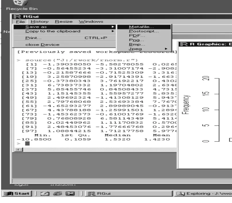
Windows

Graphs can be copied and printed using the menus on the toolbar. You make the graphics window active by clicking on its border - the border is blue, not gray, when it is active. Then click on Files on the toolbar and make your choice for printing or saving.

You can save the graphics as a .bmp file but that is bulky in terms of bytes. The .wmf format (Windows meta file) is okay for drafts.

Figure 5.1: saving a graph using Windows

You can also save graphs from the script, savePlot(file="histogram",type="bmp") or savePlot(file="histogram",type="pdf") .

5.4

Multiple Graphics windows

Suppose that you wish to have your program generate more that 1 graph. Extra graphics windows are opened by

• Linux & Mac X11() • Windows win.graph()

The first call to a plot function, e.g. plot(), hist(), boxplot() will automatically open a graphics window. If another plot function is used, the default is to overwrite the

22 CHAPTER 5. ELEMENTS OF R PROGRAMS

previous graph in the window which already exists. If you require a separate window, the program must open a new graphics device.

Example 5.1

The following job plots 2 graphs in different windows.

#_________ graphs.R _______ options(digits=2)

x <- 1:20

plot(x,log(x),type=’l’,xlab="x",ylab="log(x)")

X11() # Windows users would put win.graph()

v <- seq(-pi,pi,length=51) plot(v,cos(v),type=’b’)

dev.set(which=2) # save the plot in graphics device 2

savePlot(file="log",type="bmp")

dev.set(which=3) # save the plot in graphics device 3

savePlot(file="cos",type="bmp")

TRUE or FALSE

The arguments TRUE and FALSE are used widely and can be shortened to T and F. These letters are reserved for TRUE/FALSE and cannot be used as object names.

5.4. MULTIPLE GRAPHICS WINDOWS 23

Example 5.2

This example is to exploit the ideas of this chapter. We shall

(i) assign numbers to 2 objects, x and y using the c() function to combine values into a vector,

(ii) calculate the correlation between x and y, (iii) print the correlation in a file,

(iv) plot and save the graph of y versusx.

The example requires the user to edit T/Fdepending on their operating system (Linux or Windows). Windows users Saveor Printusing the Filesmenu.

options(digits=3) # 3 significant decimals in the output x <- c(7.51,6.72,4.83,9.21,7.57,6.38,7.80,7.25,6.67,9.46,

8.75,9.26,5.47,5.24,5.57,8.66,7.69,7.15,4.46,9.15) y <- c(38.3,35.3,25.9,48.4,41.2,33.3,40.6,38.1,36.6,49.6, 45.0,48.3,30.2,28.5,30.9,45.8,39.6,38.7,24.1,48.5) rho <- cor(x,y); print(rho)

plot(x,y)

sink("correlation.txt"); print(rho); sink()

if(T){ # for Linux users= T, Windows users= F

dev.copy2eps(file="correlation.ps",horizontal=F)

} # end of the if(T/F) statements

Note:

• Blank lines are not read by R and so are useful for spacing the program into segments. • Long lines continue on the next line, with commas to signify the continuity.

• The semi-colon means End of Line (eol). Hence you can do more than 1 command on a line if the previous is terminated by ;

Chapter 6

Troubleshooting: FAQ

by Ms J Reid

School of Mathematics, Statistics and Computer Science, U.N.E.

1. How do I locate and fix errors in my program? Some of the more common errors are:

(i) R is unable to open the data file. Refer to item 2 below. (ii) R does not recognise a variable name. Refer to item 6 below. (iii) Syntax errors:

These occur when you type your commands incorrectly: •R is case sensitive

•Don’t confuse the letter l with the numeral1.

•Check that the number of opening and closing brackets match.

Often the error message will help identify the line in your command file where the error has occurred.

Error in parse(file, n, text, prompt) : syntax error on line 9 The error on line 9 (say) may be a consequence of incomplete statements on a previous line (probably line 8 but maybe even before that), e.g. close brackets. (iv) You may have more than one variable with the same name. R will use the first variable that it encounters in the search path. Refer to § ?? of this guide for more information

25

2. R won’t read my data file. Example: Error message

> CO2<-read.table("CO2.dat",header=T)

Error in file(file, "r") : unable to open connection In addition: Warning message:

cannot open file ‘CO2.dat’

(i) Check that you have changed the directory to the one where your data file is stored (refer to page?? in this guide, Example 1, Step 4).

You can do this in R by selecting the File> Display File(s) option. Select Files of Type: All Files(*.*). If your data file is not listed then you are either not in the correct directory (Go to File> Change dir...) or you have not saved your data file to the correct directory (move your data file).

(ii) If you want to read data from a directory other than your working directory you could type in the correct path in theread.tablecommand. For example if you are in your working directory but you want to read a data file (CO2.txt, for example) from another directory (C:/data, for example) then you would type: > CO2<- read.table("C:/data/CO2.txt",header=T)

(iii) Alternatively your data may be separated by a comma or a tab delimiter rather than space. You will need to modify yourread.table command (refer to §?? of this guide).

3. How should I save my files in Notepad?

To use Notepad in Windows, go to Start>Program> Accessories> Notepad. You should save your command files using the .r extension. When saving a com-mand file in Notepad make sure that you select the File Type: All Files(*.*) option, otherwise the file will be saved with a.txtextension. Also use r in the name of the file to help distinguish it (eg. histR.rfor a command file andhist.txtfor a data file).

Data files can have different extensions but it is simplest to save data files with a .txt extension.

Refer to page ?? for further information.

4. R overwrites my graphs - how can I view previous graphs?

If you are producing a number of graphs, you may want to scroll through them to view earlier ones.

26 CHAPTER 6. TROUBLESHOOTING: FAQ

BY MS J REID

(i) Before each plotting command you could open a new graphics window. If you are using Windows:

> win.graph() In Linux: > X11()

(ii) Alternatively, in Windows open a graphics window withwin.graph()and then select the menu option History> Recording. Any plots produced will be stored and you will then be able to scroll through previous plots using thePage Upand Page Down keys.

5. When I run my command file, I do not get any output.

To run your command file (eg. rnorm.r) you select the menu option File> Source R Code or type the following:

> source("rnorm.r")

To view all output you should use the following: > source("rnorm.r",echo=T).

Refer to the end of Example 1 on page 10. 6. R doesn’t recognise a variable name.

(i) You may have typed the name in incorrectly. Remember R is case sensitive. Let’s consider a simple example: Suppose that your data contain a variable called “Rate”. In your command file you type in “rate”. You would obtain the following error message:

Error in eval(expr, envir, enclos) : Object "rate" not found

(ii) You may not have identified the data frame which the variable comes from. Refer to §?? for information about data frames.

Continuing the example above: Suppose that the variableRate is stored in the data frame datadf.

If you refer to Rate without identifying the data frame you would get an error message similar to the one above.

You have two options:

•Refer to the data frame each time you use the variable. For example, to find the mean of Rate:

> mean(datadf$Rate)

27

> attach(datadf, pos=3) > mean(Rate)

7. How do I find out about a function, its arguments, details and defaults? You should use the help function in R. For example, typing

> help(mean) or

>?mean

will produce a window with, amongst other things, a description of the function, a list of arguments that can be used with the function, a description of the output that will result, and some examples using that function.

8. How do I find a function to process data in a way that I wish?

Select the menu option: Help> Html help and then click on the Search Engine and Keywords link. You can search for keywords, function and data names and text in help page titles by typing in the relevant keywords.

You can locate other sources of information by selecting theHelp> Manualsmenu option from the R console to view manuals linked to the R site.

28 CHAPTER 6. TROUBLESHOOTING: FAQ

BY MS J REID

References

1. Ross Ihaka and Robert Gentleman 1996. ’R: A Language for Data Analysis and Graphics’, Journal of Computational and Graphical Statistics, Vol 5, No 3, pp299– 314

2. http://mcs.une.edu.au/CRAN 3. http://www.R-project.org/

4. Venables, W. and Ripley, B. 2001 Modern Applied Statistics with S-PLUS Springer, NY.

5. Dalgaard, P. 2002 Introductory Statistics with R Springer, NY. 6. Cleveland, B. (1995) Visualizing Data