Scholarship@Western
Scholarship@Western
Electronic Thesis and Dissertation Repository
11-22-2010 12:00 AM
Survival Analysis of Microarray Data With Microarray
Survival Analysis of Microarray Data With Microarray
Measurement Subject to Measurement Error
Measurement Subject to Measurement Error
Juan Xiong
The University of Western Ontario Supervisor
Dr. Wenqing He
The University of Western Ontario
Graduate Program in Statistics and Actuarial Sciences
A thesis submitted in partial fulfillment of the requirements for the degree in Doctor of Philosophy
© Juan Xiong 2010
Follow this and additional works at: https://ir.lib.uwo.ca/etd
Part of the Biostatistics Commons, Microarrays Commons, and the Survival Analysis Commons
Recommended Citation Recommended Citation
Xiong, Juan, "Survival Analysis of Microarray Data With Microarray Measurement Subject to Measurement Error" (2010). Electronic Thesis and Dissertation Repository. 34.
https://ir.lib.uwo.ca/etd/34
This Dissertation/Thesis is brought to you for free and open access by Scholarship@Western. It has been accepted for inclusion in Electronic Thesis and Dissertation Repository by an authorized administrator of
MEASUREMENT SUBJECT TO MEASUREMENT ERROR
(Spine title: Survival Analysis of Microarray Data with Measurement Error)
(Thesis format: Monograph)
by
Juan Xiong
Graduate Program in
Statistics
A thesis submitted in partial fulfillment of the requirements for the degree of
Doctor of Philosophy
School of Graduate and Postdoctoral Studies The University of Western Ontario
London, Ontario, Canada
c
SCHOOL OF GRADUATE AND POSTDOCTORAL STUDIES
CERTIFICATE OF EXAMINATION
Supervisor Examiners
Dr. Wenqing He Dr. Joseph Beyene
Dr. Duncan Murdoch
Dr. John Koval
Dr. Xingfu Zou
The thesis by
Juan Xiong
entitled:
SURVIVAL ANALYSIS OF MICROARRAY DATA WITH
MICROARRAY MEASUREMENT SUBJECT TO MEASUREMENT
ERROR
is accepted in partial fulfillment of the
requirements for the degree of
Doctor of Philosophy
Date
Chair of the Thesis Examination Board
Microarray technology is essentially a measurement tool for measuring expressions of
genes, and this measurement is subject to measurement error. Gene expressions could
be employed as predictors for patient survival, and the measurement error involved
in the gene expression is often ignored in the analysis of microarray data in the
literature. Efforts are needed to establish statistical method for analyzing microarray
data without ignoring the error in gene expression.
A typical microarray data set has a large number of genes far exceeding the
sample size. Proper selection of survival relevant genes contributes to an accurate
prediction model. We study the effect of measurement error on survival relevant
gene selection under the accelerated failure time (AFT) model setting by regularizing
weighted least square estimator with adaptive LASSO penalty. Simulation results
and real data analysis show that ignoring measurement error will affect survival
rel-evant gene selection. Simulation-Extrapolation (SIMEX) method is investigated to
adjust the impact of measurement error on gene selection. The resulting model after
adjustment is more accurate than the model selected by ignoring measurement error.
Microarray experiments are often performed over a long period of time, and
samples can be prepared and collected under different conditions. Moreover,
differ-ent protocols or methodology may be applied in the experimdiffer-ent. All these factors
contribute to a possibility of heteroscedastic measurement error associated with
mi-croarray data set. It is of practical importance to combine mimi-croarray data from
different labs or platforms. We construct a prediction AFT model using data with
heterogeneous covariate measurement error. Two variations of the SIMEX algorithm
are investigated to adjust the effect of the mis-measured covariates. Simulation
naive method.
In this dissertation, the SIMEX method is used to adjust for the effects of
co-variate measurement error. This method is superior to other conventional methods
in that it is not only more robust to distributional assumptions for error prone
covari-ates, it also offers marked simplicity and flexibility for practical use. To implement
this method, we developed an R package for general users.
Keywords: Accelerated failure time model, Measurement error, Microarray,
Predic-tion, Simulation and extrapolation method, Survival analysis, Variable selection.
All materials presented in this thesis were obtained under the supervision of Dr.Wenqing
He. Dr.He provided valuable insight in the ideas behind the materials. The majority
of the work associated with implementing this research was done by myself.
I would like to express my gratitude to my Dissertation supervisor, Dr. Wenqing He.
His encouragement, advice and support over the past five years have been tremendous,
which I appreciate from the bottom of my heart. This dissertation would not have
been possible without his support and guidance. He has helped me develop my
scientific acumen and has been a mentor in true sense.
I would also like to thank Dr. Joseph Beyene, Dr. Duncan Murdoch, Dr. John
Koval and Dr. Xingfu Zou for serving as members of my dissertation committee,
reading my dissertation thoroughly and providing very helpful comments and
sugges-tions on my research. I also want to thank Dr. Hao Yu for his technical and career
advice during my graduate study.
I would like to extend my deep appreciation to the Department of Statistical and
Actuarial Sciences at the University of Western Ontario for providing great academic
and logistic support for my graduate study. I would like to thank knowledgable faculty
members for their excellent lectures and thank friendly staff Jennifer, Lisa and Jane
for their assistance. I appreciate many colleagues in my department, especially Paul,
for his friendship and support.
Personally, I would like to express thanks to my parents for their continued love
and encourage throughout my entire life. I would also like to express thanks and
gratitude to my uncle for his love and support during my time in graduate school.
Finally, I own my thanks to Xin Song and Juanna Yang because I could not make it
through without their love, encouragement and support.
CERTIFICATE OF EXAMINATION ii
ABSTRACT iii
CO-AUTHORSHIP STATEMENT v
DEDICATION vi
ACKNOWLEDGEMENTS vii
TABLE OF CONTENTS viii
LIST OF TABLES x
LIST OF FIGURES xiii
1 Introduction 1
1.1 Microarray Technology . . . 1
1.1.1 Microarray Data Examples . . . 1
1.1.2 Genomes and Microarray Experiment . . . 3
1.2 Survival Analysis . . . 4
1.2.1 Cox Proportional Hazards Model . . . 5
1.2.2 Accelerated Failure Time Model . . . 6
1.3 Survival Analysis with Microarray Data . . . 7
1.3.1 Variable Selection . . . 7
1.3.2 Variable Selection for Survival Outcomes . . . 9
1.4 Measurement Error Models . . . 9
1.4.1 Models for the Measurement Error Process . . . 10
1.4.2 Methods for Measurement Error Analysis . . . 11
1.5 Survival Analysis with Measurement Error . . . 12
1.6 Objective of This Thesis . . . 13
Gene Expression Subject to Measurement Error 16
2.1 Introduction . . . 16
2.2 Model Framework . . . 18
2.2.1 The Adaptive LASSO Regularized Inverse Probability of Cen-soring Weight (IPW) Method . . . 18
2.2.2 Variable Selection with Mismeasured Covariates . . . 20
2.2.3 Simulation Extrapolation Method . . . 21
2.3 Simulation Studies . . . 27
2.4 Real Data Analysis . . . 36
2.4.1 PBC Data . . . 36
2.4.2 DLBCL Data . . . 39
2.5 Summary . . . 48
3 Prediction of Survival Time by Combining Mismeasured Gene Ex-pression Data from Different Platforms 49 3.1 Introduction . . . 49
3.2 Methodology . . . 51
3.2.1 Notation and Assumptions . . . 51
3.2.2 The Effect of Measurement Error and Adjustment . . . 52
3.2.3 Two Variation of the SIMEX Algorithm . . . 52
3.2.4 Best Linear Prediction and Regression . . . 54
3.2.5 Prediction Accuracy Criteria . . . 59
3.3 Simulation Study . . . 61
3.3.1 X and Z are Independent . . . 62
3.3.2 X and Z are Independent but X are Correlated . . . 65
3.3.3 Distribution ofX Depends on Z . . . 73
3.4 Conclusion . . . 78
4 simexaft: R Package for Accelerated Failure Time Models with Co-variates Subject to Measurement Error 80 4.1 Introduction . . . 80
4.2 Notation and Framework . . . 81
4.3 Simulation Extrapolation Method . . . 82
4.3.1 Implementation in R . . . 83
4.4 Examples . . . 85
4.5 Discussion . . . 91
5 Conclusion and Future Work 93 BIBLIOGRAPHY 97 A Appendices 105 A.1 R code for SIMEXAFT Package . . . 105
A.2 The Impact of Ignoring Measurement Error . . . 111
CURRICULUM VITAE 114
2.1 Survival relevant gene selection: Simulation results of independent co-variance matrix with α=1.5 and censoring rate=30%. . . 30 2.2 Survival relevant gene selection: Simulation results of independent
co-variance matrix with α=1.5 and censoring rate=50%. . . 31 2.3 Survival relevant gene selection: Simulation results of exchangeable
covariance matrix with α=1.5 and censoring rate=30%. . . 32 2.4 Survival relevant gene selection: Simulation results of exchangeable
covariance matrix with α=1.5 and censoring rate=50%. . . 33 2.5 Survival relevant gene selection: Simulation results of independent
co-variance matrix with α=0.5 and censoring rate=30%. . . 34 2.6 Survival relevant gene selection: Simulation results of independent
co-variance matrix with α=0.5 and censoring rate=50%. . . 35 2.7 Fit the AFT model to PBC data using adaptive LASSO regularzied
IPW method. ˆβx: estimate of coefficient; SE( ˆβx): the bootstrap
stan-dard error;p: the corresponding p-value. . . 37 2.8 PBC data: Sensitivity analysis with all of the quantitative covariates
subject to measurement error . . . 38 2.9 Fit the AFT model to DLBCL data: ˆβx is the estimate of coefficient,
SE( ˆβx) is the bootstrap standard error andpis the correspondingp-value. 41
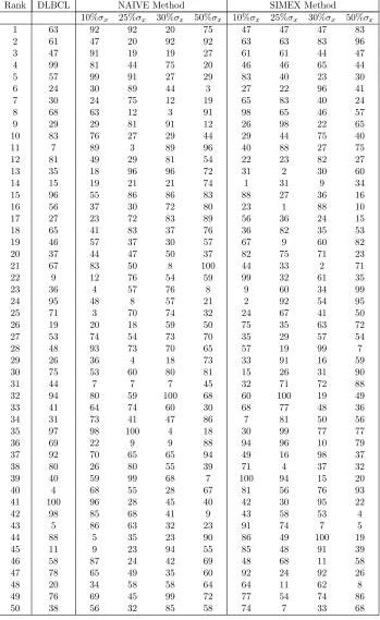
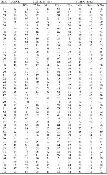
2.10 NAIVE Method: Sensitivity Analysis on DLBCL Data Set (1) . . . . 42 2.11 NAIVE Method: Sensitivity Analysis on DLBCL Data Set (2) . . . . 43 2.12 SIMEX Method: Sensitivity Analysis on DLBCL Data Set (1) . . . . 44 2.13 SIMEX Method: Sensitivity Analysis on DLBCL Data Set (2) . . . . 45 2.14 Ranks of the genes based on level of significance from the sensitivity
analysis on the DLBCL Data (1) . . . 46 2.15 Ranks of the genes based on level of significance from the sensitivity
analysis on the DLBCL Data (2) . . . 47
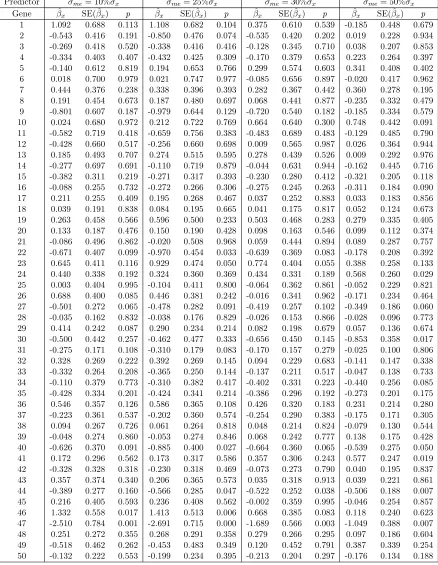
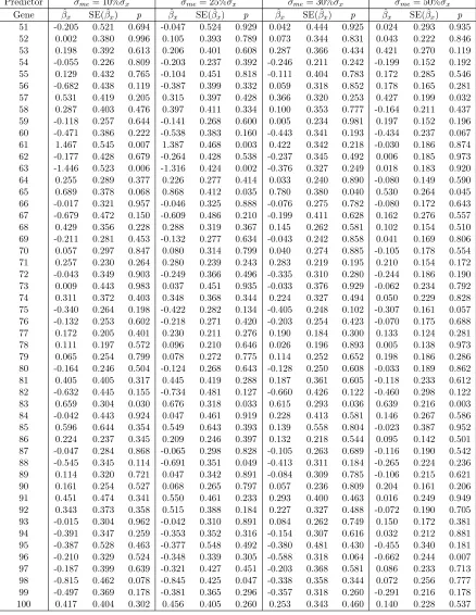
3.1 Comparison of mean squared prediction errors between the NAIVE and SIMEX methods: Variance known,x and z are independent, α= 0.5. 63 3.2 Comparison of mean squared prediction errors between the NAIVE and
SIMEX methods: Variance known,x and z are independent, α= 1.5. 63 3.3 Comparison of mean squared prediction errors: Scenario 3.1.1 . . . . 65 3.4 Comparision of mean squared prediction errors between the NAIVE
and SIMEX methods: Unknown variance, x and z are independent, α= 0.5. . . 66 3.5 Comparision of mean squared prediction errors between the NAIVE
and SIMEX methods: Unknown variance, x and z are independent, α= 1.5. . . 66 3.6 Comparison of mean squared prediction errors: Scenario 3.1.2 . . . . 67 3.7 Comparison of mean squared pridiction errors: Scenario 3.2.1 . . . 68
and SIMEX methods: Variance known, X and z are independent, the correlation betweenX is 0.8, α= 0.5. . . 69 3.9 Comparison of mean squared prediction errors between the NAIVE
and SIMEX methods: Variance known, X and z are independent, the correlation betweenX is 0.8, α= 1.5. . . 69 3.10 Comparison of mean squared prediction errors between the NAIVE
and SIMEX methods: Variance known, X and z are independent, the correlation betweenX is 0.3, α= 0.5. . . 70 3.11 Comparison of mean squared prediction errors between the NAIVE
and SIMEX methods: Variance known, X and z are independent, the correlation betweenX is 0.3, α= 1.5. . . 70 3.12 Comparison of mean squared prediction errors between the NAIVE
and SIMEX methods: Variance known, X and z are independent, the correlation betweenX is -0.3, α= 0.5. . . 71 3.13 Comparison of mean squared prediction errors between the NAIVE
and SIMEX methods: Variance known, X and z are independent, the correlation betweenX is -0.3, α= 1.5. . . 71 3.14 Comparison of mean squared prediction errors between the NAIVE
and SIMEX methods: Variance known, X and z are independent, the correlation betweenX is -0.8, α= 0.5. . . 72 3.15 Comparison of mean squared prediction errors between the NAIVE
and SIMEX methods: Variance known,X and z are independent, the correlation betweenX is -0.8, α= 1.5. . . 72 3.16 Comparison of mean squared prediction errors between the NAIVE
and SIMEX methods: Variance known, x and z are correlated, the correlation is 0.5,α = 0.5. . . 74 3.17 Comparison of mean squared prediction errors between the NAIVE
and SIMEX methods: Variance known, x and z are correlated, the correlation is 0.5,α = 1.5. . . 74 3.18 Comparison of mean squared prediction errors between the NAIVE
and SIMEX methods: Variance known, x and z are correlated, the correlation is 0.3,α = 0.5. . . 75 3.19 Comparison of mean squared prediction errors between the NAIVE
and SIMEX methods: Variance known, x and z are correlated, the correlation is 0.3,α = 1.5. . . 75 3.20 Comparison of mean squared prediction errors between the NAIVE
and SIMEX methods: Variance known, x and z are correlated, the correlation is -0.3,α= 0.5. . . 76 3.21 Comparison of mean squared prediction errors between the NAIVE
and SIMEX methods: Variance known, x and z are correlated, the correlation is -0.3,α= 1.5. . . 76 3.22 Comparison of mean squared prediction errors between the NAIVE
and SIMEX methods: Variance known, x and z are correlated, the correlation is -0.5,α= 0.5. . . 77
and SIMEX methods: Variance known, x and z are correlated, the correlation is -0.5,α= 1.5. . . 77
4.1 Extrapolation of the coefficient . . . 91
Chapter 1
Introduction
1.1
Microarray Technology
Microarray is an innovative technology that facilitates the analysis of thousands of
gene expressions simultaneously (Golub et al., 1999; Schena et al., 1995). The use of
this technology calls for a multidisciplinary efforts from biological, statistical sciences
and bioinformatics community. There have been various microarray studies carried
out in recent years.
1.1.1 Microarray Data Examples
1. DLBCL Data
Diffuse large-B-cell lymphoma (DLBCL) is the most common type of lymphoma
in adults. The data set of Rosenwald et al. (2002) consists of 7399 gene
ex-pression profiles across 240 patients with untreated DLBCL. Median survival
time was 2.8 years and 138 patients died during this follow up period. Gene
expression can be used as predictor of patient survival time after chemotherapy.
In Rosenwald et al. (2002), the authors used 17 genes to build a Cox regression
model to predict the survival time of these DLBCL patients.
2. Golub Data
The data set of Golub et al. (1999) consists of 72 bone marrow samples
ob-tained from acute leukemia patients. Ribonucleic acid (RNA) prepared from
microarray, where 6817 human gene expression profiles were measured. By
re-lying on gene expression, Golub et al. (1999) were able to make distinguishable
identification between acute myeloid leukemia (AML) and acute lymphoblastic
leukemia (ALL) without any prior knowledge of these classes.
3. Breast Cancer Data
Van de Vijver et al. (2002) studied a cohort of 295 young patients with breast
cancer. This study utilized only tumor specimens which were less than 5 cm. All
patients were treated using modified radical mastectomy or breast-conserving
surgery and assessed annually for a period of at least five years. The median
follow-up among all 295 patients was 6.7 years. The authors reported that
prediction model based on 70 gene expression profiles performed best for the
appearance of distant metastases during the first five years after treatment.
These studies give examples of the applications of microarray technology to measure
gene expression, and utilize gene expression as covariate to build statistical model for
survival prediction, group classification, etc.
Microarray is a breakthrough technology that allows us to analyze completed
genetic variations in entire genome level (Golub et al., 1999). Introduced in the
mid-1990s (Schena, 1995; Lockhart, 1996; DeRisi, 1997), microarray has ever since been
applied to a number of diverse areas, such as nutrition research (DellaPenna, 1999),
drug discovery (Debouck, 1999), environmental health research (Nuwaysir, 1999) and
cancer diagnostic (Golub, 1999; Dudoit, 2002). With the advent of new
technolo-gies and more rapid methods of analysis, microarray technology has the potential to
become increasingly popular tool in many new areas in the future. Comprehensive
reviews of microarray technology and data analysis can be found in Duggan et al.
(1999) and Quackenbush (2001, 2002).
Microarray technology is essentially a measurement tool for measuring biological
be subject to error, and those measurement errors are often ignored in the microarray
data analysis in the literature. We investigate this issue in this thesis.
1.1.2 Genomes and Microarray Experiment
To provide a better picture of gene expression data, we give a brief background of
the gene and procedures of microarray experiment. Genes are hereditary units that
are composed of deoxyribonucleic acid (DNA) sequences organized in chromosomes in
the cell nucleus (Russell et al., 2009). The DNA sequences control the generation of
messenger ribonucleic acids (mRNA) through a process called transcription. mRNA
encodes amino acids that subsequently form proteins through a process called
trans-lation. The proteins carry out the designated function of a particular gene. Thus, the
structural and functional features of cells and tissues are determined by the
simul-taneous, selective, and differential expressions of thousands of genes. The type and
amount of protein present in the cells determine the phenotypes of the cells, such as
cancer or normal cells.
A microarray is a solid substrate (usually glass) upon which many different
cD-NAs have been spotted in specific locations in a grid pattern. mRNA from a tissue
sample of interest is extracted and the reverse transcription is applied to synthesize
cDNA, and labels the cDNA with fluorescent dye or radioactive nucleotides. This
la-beled cDNA is then hybridized to cDNA immobilized on the array. The lala-beled cDNA
binds to its complementary sequence approximately proportional to the amount of
each mRNA transcript in a sample. The amount of radioactivity or fluorescence can
be measured, allowing estimation of the amount of mRNA for each transcript in the
sample. Once a microarray experiment has been conducted, the arrays are scanned
by a confocal laser microscope. The images from the scanner are processed to extract
the spot intensities and background spot intensities. The gene expression levels are
measured by the normalized ratio of the fluorescence intensity of the test sample and
from multiple platforms, it is worth to point out that our methods are not limited to
specific platforms, as long as the generated data are continuous variable. In the case
of the SNP microarray platform, a log transformation is sufficient to convert discrete
variables into continuous variables, so to satisfy prerequisite of our methods.
1.2
Survival Analysis
Survival analysis or time-to-event data analysis is a branch of statistics which
empha-sizes on developing statistical methods for analyzing the time to an event of interest,
often referred to as survival time or failure time (Lawless, 2003). Survival analysis is
an important topic in various scientific fields, such as biomedical sciences, economics
and engineering. One special characteristic of survival data is that the survival time
may be subject to censoring. Censoring generally occurs because subject may be lost
in the follow-up during the study period or withdraw from the study due to death or
some other reasons. In this thesis, we will focus on right censoring. Suppose that we
have a random sample ofn subjects,i= 1, . . . , n. LetTi be the survival time and Ci
be the censoring time. Usually, it is assumed that the survival time is independent of
the censoring time, or at least that they are independent given certain covariates. We
only observe min(Ti, Ci) and δi =I(Ti ≤ Ci) is the censoring indicator, with δi = 0
if subject i is censored and δi = 1 if the survival time Ti is observed.
The survival function and hazard function are essential to survival analysis. The
survival function, S(t), describes the probability that the random variate T exceeds
the specified time t and is given by
S(t) =P r(T ≥ t) for t≥ 0,
where S(t) is non-increasing and left continuous. At time t = 0, S(0) = 1 and at
The hazard function, h(t), gives the instantaneous rate of failure at time t on
condition that individual surviving up to t and is given by
h(t) = lim
∆t→ 0
P r(t ≤ T < t+ ∆t|T ≥ t)
∆t .
In contrast to the survival function, the hazard function focuses on failure given
survival up to a certain time point. The hazard function can be used to identify the
form of model. The relationship between S(t) and h(t) is
S(t) = exp
−
Z t
0
h(u)du
.
1.2.1 Cox Proportional Hazards Model
Cox proportional hazards (PH) model is one of the most popular semiparametric
regression model in survival analysis (Cox, 1972). The Cox PH model is given by
h(t|Xi) = h0(t) exp (X0iβx),
where h0(t) is a unspecified baseline hazard function; Xi = (Xi1, Xi2, . . . , Xip)0 is p
dimensional vector of covariates andβxis the associated vector of unknown regression
coefficients, which can be estimated by maximizing the partial likelihood (Cox, 1975)
L(βx) =
n
Y
i=1
eX0iβx
P
j∈ Ri
eX0jβx
δi
,
where Ri is the risk set of subjects at timeti given by
1.2.2 Accelerated Failure Time Model
Another attractive alternative to the Cox PH model is the accelerated failure time
(AFT) model (Kalbfleisch and Prentice, 1980). The AFT model relates the logarithm
of the survival time linearly to covariates and is given by
Yi =β0+X0iβx+i, (1.1)
where Yi = log (Ti), i is the error term. The parametric AFT model specifies
the distribution of i up to parameters α. Common choice of distribution include
the Weibull, exponential, Gaussian, logistic, log-normal and log-logistic distribution
(Lawless, 2003). The semiparametric AFT model does not make any assumption on
the distribution of i.
The Cox PH model and AFT model are intended for different types of
com-parisons (i.e., the Cox PH model compares the hazard functions whereas the AFT
model compares the survival times). In the Cox PH model, the covariates are
mul-tiplicative to the hazard function and remains constant over time, whereas in the
AFT model, the covariates are multiplicative to the survival times. Compared to the
Cox PH model, the results of AFT models are easier to interpret due to its direct
modeling of the survival time (Reid, 1994). Also, when there is no censoring, the
AFT models reduce to ordinary generalized linear regression models. AFT models
have been studied extensively in the literature: Miller (1976) and Buckley and James
(1979) modified the least square estimate equation to account for the censored
re-sponse variable; Tsiatis (1990) and Ying (1993) proposed the rank based estimator;
and Stute (1996) investigate the weighted least square estimator. In this thesis, we
1.3
Survival Analysis with Microarray Data
Central to the application of microarrays in biomedical and genomic research is to
re-veal different gene expression profiles under different medical or treatment scenarios.
For example, in cancer research, gene expression profiles can help further
understand-ing of cancer at the genetic or molecular level.
With the microarray features of each patient, we can have a patient survival
prediction model that is biologically meaningful. Microarray experiments generate
large data sets, to which many biological researchers may not be accustomed (Page
et al., 2003). A typical microarray data set has a large number of genes far exceeding
the sample size. Other than the high dimensionality of the genes, the expression levels
of genes are often highly correlated. As a pre-procedure, one needs to identify survival
relevant genes from a large set of candidates produced by microarray experiments.
After identifying a subset of genes with the most predictive power to the survival
outcome of the patient, one can combine them with patient specific covariates to
build a prediction model for future patients’ survival outcomes. Simply put, proper
selection contributes to an accurate prediction model that are both clinically and
biologically meaningful, and could lead to better treatment choice for patients.
1.3.1 Variable Selection
Variable selection is fundamental in statistical modeling and data analysis.
Tra-ditional variable selection approaches include Akaike information criterion (AIC)
(Akaike, 1973), Bayesian information criterion (BIC) (Schwarz, 1978), and risk
infla-tion criterion (RIC) (Foster and George, 1994). Recent high throughput technologies
have generated data where the number of covariates is significantly larger than the
sample size. Typical examples include microarray data, text categorization and image
retrieval. New features of these data present a direct challenge to standard variable
Literature on variable selection in high dimensional models is growing quickly.
Fan and Lv (2010) presented a review on variable selection in high-dimensional
mod-eling. Here we introduce two popular methods: least absolute shrinkage and selection
operator (LASSO) (Tibshirani, 1996) and the adaptive LASSO (Zou, 2006).
1.3.1.1 LASSO
Tibshirani (1996) proposed the popular shrinkage regression technique that could
select variables and estimate the regression coefficient simultaneously. The LASSO
estimate is defined as
b
βx(lasso) = argmin βx
n
X
i=1
Yi−
p
X
j=1
Xijβxj
2
+ γ n
p
X
j=1
βxj
,
where Yi is the response for subject i, Xi = (Xi1, Xi2, . . . , Xip)0 is p dimensional
covariate vector and βx is the associated vector of unknown regression coefficients.
γ is a penalty parameter determined by cross-validation. It shrinks a number of
coefficients to zero, thus can be used for variable selection. Efron et al. (2004)
published least angle regression algorithm which can be employed to solve LASSO
estimate.
1.3.1.2 Adaptive LASSO
Fan and Li (2001) showed that the LASSO penalty produces biased coefficients
es-timates. To overcome the bias, Zou (2006) proposed the adaptive LASSO that has
oracle properties:“ it can not only selects significant variables consistently but also
performs as efficient as if the true model was known, a property not enjoyed by the
LASSO.” Hence, the adaptive LASSO method is an ideal one for variable selection.
b
βx= argmin βx
n
X
i=1
Yi−
p
X
j=1
Xijβxj
2
+γ p
X
j=1 vj
βxj
,
wherev= (v1, . . . , vp) is a known weight vector. The weight vector can be constructed
as v = 1/|β∗ |τ, τ > 0, where β∗ needs to be a root-n-consistent estimator of βx, such as the ordinary least square estimate.
1.3.2 Variable Selection for Survival Outcomes
In the past few years, some of the variable selection procedures in linear regression
analysis have been extended to the censored survival data analysis in the presence of
high dimensional predictors. For example, Tibshirani (1997) developed a regularized
Cox regression by minimizing L1 LASSO penalty to the partial likelihood; Faraggi
and Simon (1998) proposed a Bayesian variable selection method for the Cox model;
Li and Luan (2003) investigated the L2 penalized estimation of the Cox model using
kernel; and Gui and Li (2005) introduced a threshold gradient descent regularization
estimation method. For the AFT model, Schmid and Hothorn (2008) presented a
boosting algorithm for fitting the parametric AFT model. For the semiparametric
AFT model, Huang et al. (2006) investigated the LASSO regularization for estimation
and variable selection in the AFT model based on the inverse probability of censoring
weights method; Huang and Harrington (2005), Datta et al. (2007) used the LASSO
regularized Buckle-James method for the AFT model; and Cai et al. (2008) developed
variable selection for the AFT model by the LASSO regularized rank based estimator.
1.4
Measurement Error Models
In many biomedical studies, it is often the case that some covariates can not be
measured accurately, which leads to measurement error models or errors-in-variable
reasons. Sometimes it is due to covariate nature, for instant, blood pressure. In other
cases the patient consent and cost may prevent precise observation of the covariate.
It is well known that ignoring measurement error in covariate leads to biased estimate
of the covariate effects and consequently affects inference (Fuller, 1987; Carroll et al.,
2006).
In the past several decades, a great deal of research has been done on
mea-surement error models. Fuller (1987) summarized a detailed discussion of statistical
method for linear measurement error models while Carroll et al. (2006) provided
systematic guide on dealing with nonlinear measurement error models. Recently, the
study of measurement error models has become an increasingly popular theme in
nonparametric measurement error area (Delaigle and Meister, 2007; Carroll et al.,
2009).
1.4.1 Models for the Measurement Error Process
Specifying the model for the measurement error process is fundamental for
analyz-ing measurement error problems. There are a number of measurement error models
reported in the literature. The general two models are the classical additive
measure-ment error model and the Berkson error model. Assume we have response Yi and
two types of covariates,Zi consists of the covariates measured without error, and Xi
represents those that can not be observed exactly for subjects i = 1, . . . , n. Instead
of observing Xi, we observe its contaminated version Wi.
The classical additive model assumes that
Wi =Xi+Ui, (1.2)
the Berkson model assumes that
where measurement error Ui has multivariate normal distribution with mean 0 and
variance Σui. The measurement errors can be either homoscedastic or
heteroscedas-tic. If the variances Σui are the same for all subjects, it is called homoscedastic
measurement error. Otherwise it is heteroscedastic. The measurement errors are
mu-tually independent and are independent of {Yi,Xi,Zi}. The use of different model forms is decided by the nature of study.
It is important to identify distinct measurement error mechanisms.
Measure-ment error is non-differential when the distribution of Yi given (Xi,Zi,Wi) is the
same as the distribution given (Xi,Zi). In other words, Wi contains no information
about Yi other than what is available in (Xi,Zi). Wi is called a surrogate for Xi.
Otherwise, measurement error is differential. This thesis focuses on nondifferential
measurement error models.
1.4.2 Methods for Measurement Error Analysis
A large number of methods has been proposed to deal with measurement error
prob-lems, including likelihood based methods (Stefanski and Carroll, 1990); score function
methods (Kukush and Schneeweiss, 2004); Bayesian methods (Clayton, 1992); and
semiparametric and nonparametric methods (Huang and Wang, 2000). Two widely
applicable methods for measurement error analysis are regression calibration and
sim-ulation extrapolation (SIMEX).
1.4.2.1 Regression Calibration
Regression calibration is commonly applied to account for measurement error (Carroll
et al., 2006). It reduces bias in the estimate of parameter and enjoys simplicity in
practical use. This method replaces the unobserved covariate Xi by the conditional
or sandwich method is needed to adjust the standard errors of the parameter
esti-mates to account for the variation induced by estimation of parameters in modeling
E(Xi|Zi,Wi). The key issue with this method is how to best estimate this
expecta-tion.
1.4.2.2 Simulation Extrapolation Method
Cook and Stefanski (1994) introduced a SIMEX approach for estimating and
cor-recting bias due to measurement error. The general idea of the SIMEX method is
to generate additional data sets with increasingly larger measurement error, estimate
the trend of the effect of the measurement error on the estimation of the parameter
of interest. We then extrapolate the trend back to the case of no measurement error.
The major advantage of the SIMEX method is its easy implementation and
robust-ness to distributional assumptions for error prone covariates. See section 2.2.3 for the
detailed description.
1.5
Survival Analysis with Measurement Error
A well-known challenge associated with survival data analysis is to find an appropriate
way of handling measurement errors which are frequently present in covariates. It
is known that many biomarkers, such as blood pressure and CD4 counts are often
subject to measurement error. Great research effort has already been undertaken to
explore effective ways of handling covariate measurement error for survival data.
Prentice (1982) first considered the regression calibration method to adjust the
impact of measurement error in covariates for the Cox PH model; Clayton (1992)
modified Prentice’s approach by using the regression calibration within each risk set;
Zhou and Pepe (1995) proposed a nonparametric method for discrete covariates with
measurement error; later, Zhou and Wang (2000) extended this method to
developed a full likelihood approach to account for measurement error in the Cox
regression model with a single covariate; Nakamura (1992) and Buzas (1998) applied
the corrected score function to the Cox PH model when the measurement errors are
additive and normally distributed; Huang and Wang (2000) modified the score
func-tion and proposed a nonparametric approach to estimate the parameter of the Cox
regression model when replicates of Wi are available for each subject; and Gimenez
et al. (1999, 2006) have applied the corrected score approach in their investigation of
inference methods under Weibull regression models.
For multivariate survival analysis with mismeasured covariates, Li and Lin
(2000) used the expectation-maximization algorithm to calculate the
nonparamet-ric maximum likelihood estimates for clustered survival data with covariates subject
to frailty measurement error; Hu and Lin (2004) proposed semiparametric regression
methods for multivariate failure times; and Green and Cai (2004) explored the SIMEX
method in dealing with measurement error effect on multivariate failure time model.
In the above literature, all the works are focused on the Cox PH models with
covariates subject to measurement error. With AFT models, Tseng et al. (2005)
considered the joint modeling of failure time and longitudinal data under the AFT
assumption when covariates are assumed to follow a linear mixed effects model with
measurement errors; He et al. (2007) applied the SIMEX method to adjust the effect
of mismeasured covariates in the accelerated failure time model; Yu and Nan (2009)
considered the regression calibration estimation method for the semiparametric AFT
model with covariates subject to measurement error.
1.6
Objective of This Thesis
Like other measurement tools, the gene expression levels measured from microarrays
have measurement error. Throughout the microarray experiment process,
the fluorescent signal, slide hybridization, image creating and reading, etc. As
com-monly acknowledged, the presence of measurement error leads to substantially biased
and inconsistent parameter estimates. Thus this leads to invalid hypothesis test and
mask the feature of the data.
To the best of our knowledge, most existing variable selection procedures are
limited to directly observed predictors. Variable selection for measurement error
data has not been systematically studied yet. Liang and Li (2009) proposed a class
of variable selection procedures for partially linear measurement error models by
using penalized least squares and penalized quantile regression. Ma and Li (2010)
discussed variable selection for general parametric and semiparametric measurement
error models via penalized estimating equations. In this thesis, we study the impact
of measurement error on survival relevant gene selection under the AFT model.
Microarray experiments are often performed over a long period of time, and
samples can be prepared and collected under different conditions. Moreover,
differ-ent protocols or methodology may be applied in the experimdiffer-ent. All these factors
contribute to a possibility of heteroscedastic measurement error associated with
mi-croarray data set. It is of practical importance to combine mimi-croarray data from
different labs or platforms which presents a natural way to increase sample size so
that reliable statistical analysis can be conducted. In this thesis, we will
investi-gate prediction of survival time under AFT model with gene expression subject to
heteroscedastic measurement error.
An outline of this thesis is as follows. In Chapter 2, we study the effect of
measurement error on survival relevant gene selection under the AFT model setting
by regularizing the weighted least square estimator with an adaptive LASSO penalty.
In Chapter 3, we consider prediction of AFT model using data with heteroscedastic
covariate measurement error. Two variations of the SIMEX algorithm are
investi-gated to adjust the effect of the mis-measured covariates, and a best linear prediction
fu-ture observation. We develop an R package simexaft to adjust biases induced by
covariate measurement error under AFT models and illustration is given in Chapter
4. Concluding remarks and discussion on future work are presented in Chapter 5.
The source code for the R package and some technical details are included in the
Chapter 2
Survival Relevant Gene Selection in Microarray Data
Analysis with Gene Expression Subject to Measurement
Error
2.1
Introduction
Microarray technology has become a very popular tool for investigating molecular
fea-tures of different clinical outcomes (Golub et al., 1999; Dudoit et al., 2002; Rosenwald
et al., 2002). In survival analysis, microarray data are commonly used for building
a prediction model of survival outcomes based on the gene expression profiles (e.g.,
survival times of patients). However, because of their unique features, microarray
data must be analyzed carefully. For instance, the number of genes far exceeds the
sample size in many microarray data sets. Other than the high dimensionality of the
genes, the gene expression levels are often highly correlated. Therefore, we need to
identify a subset of genes that are significantly correlated with the survival outcomes,
and combine patient specific covariates together to build a prediction model for future
patients’ survival outcomes (Li, 2008).
There has been extensive research on variable selection and estimation
method-ologies in the presence of high dimensional predictors. Examples include bridge
re-gression (Frank and Friedman, 1993); non-negative garrote (Breiman, 1995); least
absolute shrinkage and selection operator (LASSO) (Tibshirani, 1996); smoothly
clipped absolute deviation (Fan and Li, 2001); gradient directed regularized method
(Friedman and Popescu, 2004); the boosting algorithm (Buhlmann and Yu, 2003);
the elastic net (Zou and Hastie, 2005); the adaptive LASSO (Zou, 2006); and the
Dantzig selector (Candes and Tao, 2007). Fan and Lv (2010) gave a comprehensive
It becomes more complicated if the goal is to predict survival time with high
dimensional gene expressions when the survival time is censored. As a consequence,
direct employment of traditional survival analysis techniques is difficult to obtain
accurate parameter estimates. See section 1.3.2 for the literature review on variable
selection methods for combining high-dimensional covariates to predict failure time
outcomes.
Microarray technology allows for the measurement of the expressions of
thou-sands of genes simultaneously. Like many other quantitative tools, gene expressions
are subject to measurement errors. It is commonly acknowledged that ignoring
mea-surement error could lead to substantially biased estimates of the regression
parame-ters (Fuller, 1987; Carroll et al., 2006). This leads to incorrect results for statistically
identifying survival relevant genes. Consequently, it is essential to investigate survival
relevant gene selection when the gene expressions are subject to measurement errors.
Huang et al. (2006) used censoring weights for adjusting the LASSO penalized
least squares loss function for variable selection in AFT model. Because of the L1
penalty structure, this method has the advantage of carrying variable selection and
estimating parameters simultaneously. The adaptive LASSO (Zou, 2006) is similar
to LASSO in that it has retained the near-minimax optimality and can be solved by
the least angle regression algorithm (Efron et al., 2004). Furthermore, it enjoys the
oracle properties as mentioned in Section 1.3.1.2.
In this chapter, we study the effect of the measurement error on survival
rel-evant gene selection in the AFT model by regularizing the weighted least square
estimator with the adaptive LASSO penalty. The bootstrap method, which samples
with replacement from the original observations, is employed to estimate variances.
The simulation extrapolation (SIMEX) method is explored to adjust the effect of
2.2
Model Framework
Survival regression models are mainly used to identify covariates that are significantly
related to the survival times. With microarray data, we use gene expressions to build
the survival model to find gene expressions that significantly predict the survival
time of a patient. Typically, the gene expression measurements from microarray
experiments have measurement errors. LetWi be the measured gene expression and
Xi be the true gene expression, which is usually unavailable, for theith subject. The
relationship betweenWi andXi could be assumed through the most commonly used
additive measurement model given by equation (1.2), where measurement error Ui
follows a normal distribution with mean 0 and covariance matrix Σui. By ignoring Ui, the AFT model (1.1) will be the naive model given by
Yi =β0+Wi0βw+i. (2.1)
The estimates for βw will attenuate from the true βx in the model (1.1) (Fuller,
1987); hence, the survival relevant variable selection will be affected (Carroll et al.,
2006; He et al., 2007).
2.2.1 The Adaptive LASSO Regularized Inverse Probability of
Censoring Weight (IPW) Method
One problem in utilizing the adaptive LASSO for survival relevant gene selection is
that the survival times are not available for censored observations. Thus, the least
square term in adaptive LASSO has to be modified for survival data. The IPW
method is a popular choice to overcome this problem (Huang et al., 2006).
only at the uncensored point by the jumps π0nis given by
πn1 = δ(1)
n ,
and
πni = δ(i) n− i+ 1
i−1
Y
j=1
n− j n− j+ 1
δ(j)
, i= 2, . . . , n,
where δ(1), δ(2), . . ., δ(n) are the censoring indicators for the corresponding ordered
logarithm of survival times Y(1) ≤ Y(2) ≤ · · · ≤ Y(n). The weighted least square estimator defined by Stute (1996) is the set of values for (β0,βx) that minimizes
`(β0,βx) =
1 2
n
X
i=1 πni
Y(i)− β0− X0(i)βx
2
,
where X(1), X(2),. . ., X(n) are covariates of the corresponding ordered Y(i)’s.
We first adjust X(i) and Y(i) by their πni−weighted means, respectively,
Xπ(i)=π1/2ni X(i)− X¯π
and
Yπ(i) =πni1/2Y(i)− Y¯π
,
where
¯
Xπ =
n
X
i=1
πniX(i)/ n
X
i=1 πni
and
¯ Yπ =
n
X
i=1
πniY(i)/ n
X
i=1 πni.
the weighted least squares (LS) objective function becomes
`(βx) = 1 2
n
X
i=1
Yπ(i)− X0π(i)βx2.
Then, the adaptive LASSO regularized IPW estimator, βbx, is the solution that
min-imizes
`(βx) = 1 2
n
X
i=1
Yπ(i)− X0π(i)βx2 +γ p
X
j=1 vj
βxj
, (2.2)
where γ is the adaptive LASSO penalty parameter and v = (v1, . . . , vp) is a known
adaptive LASSO weight component. We use v= 1/|βˆ|, where ˆβ is the ordinary least square estimate of βbx, as suggested by Zou (2006).
For the variance estimates ofβbx, we use the bootstrap method, where samples
are generated with replacement from the original observations. The bootstrap
esti-mator is computed with the same optimal value of γ as used on the original data.
According to Theorem 2 in Zou (2006), βbx is asymptotically normal.
2.2.2 Variable Selection with Mismeasured Covariates
Throughout the microarray experiment process, measurement error might be
pro-duced from various sources (He et al., 2007). Consider the hypothesis test for
evalu-ating the significance of the covariate, Xij, given by
H0 :βxj = 0 versus HA :βxj 6= 0, j = 1, . . . , p.
The test statistic is given by
zxj =
b
βxj
SE(βbx
j)
,
where βbx
j and SE(βbxj) are the estimate and standard error estimate ofβxj,
but Xij is not observable, the naive test statistic is given by
zwj =
b
βwj
SE(βbw
j)
,
whereβbw
j and SE(βbwj) are the estimate and standard error estimate of βwj,
respec-tively.
Typically, βbw
j will be attenuated from βbxj and its corresponding SE(βbwj) will
be smaller than SE(βbx
j) under certain conditons(Buzas et al., 2005). Hence, its
corresponding p-value will be different from the p-value if Xij is observable, often
leading to incorrect decisions for the hypothesis test.
A common problem for microarray data involves the analysis of high
dimen-sional gene expression data that are typically characterized by thousands of variables
with few observations. That is, these data have a high degree of multicollinearity in
the analysis. In general, the naive test statistic which ignores the measurement error
and substitutes Wi for Xi in a test is not correct (Carroll et al., 2006). Here the Xi
are highly correlated, under the multivariate distribution, the naive test of no effect
due to any component of Xi is not correct. We will use the SIMEX method (Cook
and Stefanski, 1994) to adjust the effect of measurement error on survival relevant
gene selection.
2.2.3 Simulation Extrapolation Method
Here we describe the SIMEX method to correct the bias due to measurement error.
More details are available in Carroll et al. (2006). Although the theory of the SIMEX
method is not trivial, an example from simple linear regression can well illustrate the
idea of this method. Suppose the response variableY and the covariateX is modeled
as
where has mean 0. Here X is normal distributed with variance σx2. If replacing X
with its observed measurementW, modeled by W =X+U, where U follows normal
distribution with mean 0 and variance σu2 , and is independent of and X, then the
resulting least squares estimator ˆβx∗ for βx converges in probability to
βx∗ = σ
2 x σx2 +σu2βx,
instead ofβx. To see how the bias may be related to the degree of measurement error
inX, we perturbW by adding additional error to createW(b, λ) =W+√ λUb where Ub is independently generated from a N(0, σu2) distribution. Intuitively, if regressing
Y over the perturbed version W(b, λ), then the resulting estimator ˆβx(b, λ) would
converge in probability to
βx∗ (b, λ) = σ
2 x
σ2x+ (1 +λ)σu2βx.
This expression indicates the dependence of the asymptotic bias on the magnitude
of measurement error - the less degree of measurement error (equivalently, a smaller
λ), the smaller asymptotic bias. In particular, if λ shrinks to 0, ˆβx(b,0) recovers the
naive estimator ˆβx∗ ; if λtakes value -1, then the limitβx∗ (b,−1) is identical to the true parameter βx.
We consider two practical cases for the parameters in Σui: (i) the parameters
in Σui are given as fixed values; and (ii) the parameters in Σui are not known, but
replicate measurements of Wi are available.
Suppose that one could estimate regression parameterθ by solving an
estimat-ing equation given by
0=
n
X
i=1
ϕ(θ;Yi,Xi). (2.3)
the estimates and associated variances of the parameters θ can be obtained by the
following SIMEX algorithm.
2.2.3.1 Case I: The parameters in Σui are given as fixed values.
1. Simulation Step
We generate the pseudo errors Ubi ∼ MVN(0,Σui) for i = 1, . . . , n, b =
1, . . . , B. For each λ∈ Λ, let the pseudo data be given by
Wi(b, λ) =Wi+λ
1 2Ubi.
Note that E(Wi(b, λ)|Xi) = Xi and Var(Wi(b, λ)) = Σwi(b, λ) = Σx+ (1 + λ)Σui. When λ=−1,Σw =Σx. Hence, the mean square error, E[(Wi(b, λ)− Xi)2|Xi], converges to zero as λ → − 1. This implies that Wi(b, λ) is the best
measurement of Xi. This is the most important property of the pseudo data
(Carroll et al., 2006).
2. Estimation Step
Given λ and b, we obtain the estimate bθ(b, λ) by solving equation (2.3) with
Xi replaced by Wi(b, λ). The corresponding variance estimate, Ωb(b, λ), is the
diagonal elements of the observed information matrix given by
"
−
n
X
i=1 ∂
∂θ0 ϕ(θ;Yi,Wi(b, λ))|θ=bθ(b,λ) #−1
.
By averaging over b, we obtain
b
θ(λ) =B−1 B
X
b=1
b
and
b
Ω(λ) = B−1
B
X
b=1
b
Ω(b, λ).
Define bS(λ) = (B − 1)−1
B
P
b=1
b
θ(b, λ)− bθ(λ) 2
, the variance for the estimator
b
θ(b, λ) is given by
b
Ω(λ)− Sb(λ).
3. Extrapolation Step
Fit these average estimates to an extrapolation function of lambda and
extrap-olate bθ(λ) back to the case of no measurement error (i.e., λ=−1) to yield the SIMEX estimateθbsimex. The variance estimate for bθsimex can be obtained by
extrapolating Ωb(λ)− bS(λ) back to λ=−1.
The most commonly used extrapolation functions are linear extrapolation
tion, quadratic extrapolation function and rational linear extrapolation
func-tion. The quadratic extrapolant function in the SIMEX method is generally a
safe choice for most regression models (He et al., 2007).
2.2.3.2 Case II: The parameters in Σu are not known, but replicate
mea-surements of Wi are available.
Consider the case where the measurement error covariance matrices are not known but
replicate measurements ofWi are available. The procedures of the SIMEX algorithm
described above can be applied except for the data simulation step. Devanarayan and
Stefanski (2002) introduced this variation and named it empirical SIMEX.
Suppose we have ki ≥ 2 replicate measurements denoted by {Wi1, . . . ,Wik
i}
for every subject i such that
whereUij are mutually independent from each other and independent of{Yi,Xi}. For fixedi, Uij are independent and identically distributed random errors such that Uij
iid
∼ MVN(0,Σui). Without knowing the covariance matrix Σui, we cannot generate
pseudo errors directly. However, we can obtain them by taking linear combination of
the replicated measurements.
The empirical SIMEX algorithm is as follows
1. We generate zb,i,jiid∼ N(0,1), i= 1, . . . , n, j = 1, . . . , ki, b= 1, . . . , B. We define ¯
zb,i,. =Pki
j=1zb,i,j/ki and
cb,i,j = q zb,i,j− z¯b,i,.
Pki
j=1 zb,i,j − z¯b,i,.
2
,
where Pki
j=1cb,i,j = 0 andP
ki
j=1c2b,i,j = 1.
2. For i= 1, . . . , n,j = 1, . . . , ki, b= 1, . . . , B and each λ∈ Λ, we define
Wi(b, λ) = ¯Wi.+
λ ki
12 ki X
j=1
cb,i,jWij,
where ¯Wi. = Pki
j=1Wij/ki. It is easy to see that E(Wi(b, λ)|Xi) = Xi and
Var(Wi(b, λ)) =Σwi(b, λ) = Σx+ (1 +λ)Σui/ki.
This pseudo data have the same important property as the SIMEX algorithm
defined in the previous section. That is, as λ → − 1, E[(Wi(b, λ)− Xi)2|Xi] converges to zero. We estimate bθ(b, λ) by solving equation (2.3) with Xi
re-placed by Wi(b, λ) for each b and λ. Then, we averaged over b to obtain
b
θ(λ) =PB
b=1θb(b, λ)/B.
For practical use, choosing B = 50, 100 or 200, and taking Λ to be equally
cut points of interval [0,1] or [0,2] with M = 5, 10 or 20 can often lead to fairly
reasonable SIMEX estimates (Carroll et al., 2006).
2.2.3.3 Asymptotic Normality of SIMEX Estimate
The adaptive LASSO regularized IPW method is utilized to select the variable and
estimate the covariate coefficients under the AFT setting (2.1). Here we assume that
all the covariates are subject to measurement error and the SIMEX method is applied
to adjust the effect of measurement error on variable selection on AFT models. For
each λ and b. We obtain estimates, βbx(b, λ), by minimizing
`(βx(b, λ)) = 1 2
n
X
i=1
Yπ(i)− Wi(b, λ)π(i)0 βx(b, λ)2 +γ p
X
j=1 vj
βxj(b, λ) .
For any givenλ, by applying Theorem 2 of Zou (2006), we have
√
nβbx(b, λ)− βx(b, λ)
→ d MVN(0,C(b, λ)),
where βx(b, λ) is the true unknown adaptive LASSO regularized IPW parameter.
C(b, λ) is the variance parameter. We calculate the average of these B estimators,
b
βx(λ) =B−1PB
b=1βbx(b, λ), and let C(λ) = B−1 PB
b=1C(b, λ)). According to
Slut-sky’s theorem, we have
√
nβbx(λ)− βx(λ)
→ dMVN(0,C(λ)).
Let βbx(Λ) = vec{βbx(λ);λ ∈ Λ}, βx(Λ) = vec{βx(λ);λ ∈ Λ} and Γ(Λ) = diag{C(λ), λ∈ Λ}, we have
√
n
b
βx(Λ)− βx(Λ)
Assume that the exact extrapolation functionG(ζ;λ) is known in the
extrapo-lation step to fitβbx(λ), where ζ is d-dimensional vector of parameters. Let bζ be the
least squares estimator. Let Gζ(ζ;λ) = (∂/∂ζ)G0(ζ;λ),
s(ζ) = (Gζ(ζ;λ1)Gζ(ζ;λ2)· · ·Gζ(ζ;λM))
and A(ζ) =s(ζ)s0(ζ) be the d× d matrix. Then by the similar argument to that of Carroll et al. (1996), we obtain
√
n(bζ − ζ)→ d MVN(0,Q(ζ)),
where Q(ζ) = [A(ζ)]−1s(ζ)Γ(Λ)s0(ζ)[A(ζ)]−1 is a d× d matrix. Letting λ = −1 leads to the SIMEX estimator βbx =G(bζ;−1). Therefore, obtain
√
n(βbx− βx)→ dMVN(0,Gζ0 (ζ;−1)Q ζ)Gζ(ζ;−1)
.
2.3
Simulation Studies
This section investigates the impact of ignoring measurement error on survival
rel-evant gene selection in the AFT model and exploring how the SIMEX method can
adjust the selection when measurement error is shown. Each simulation study
con-sists of 100 data sets of sizen= 200. The survival times are generated from the model
(1.1) using β0 = 0, βx = (0.7,0.7,0,0,0,0.7,0,0,0)0 and i follows the standard
ex-treme value distribution with its scale parameter,α, set to 0.5 and 1.5. The censoring
times are generated such that the censoring rates are approximately 30% and 50%.
The true covariates Xi = (Xi1, Xi2, . . . , Xi9)0 are generated from MVN(1,Σ) where
Σis defined by
Σ=
1
1 . ..
1
9×9
Scenario 2: Exchangeable Covariance Matrix
Σ=
1 ρ
ρ 1 . .. . .. ... ρ
ρ 1
9×9
where ρ, which is set to be 0.5 to account for moderate correlation, is the pairwise
correlation between Xii and Xi(i+1). The pseudo errors Ubi are generated from
MVN(0, σ2I), whereIis the identity matrix and σis set to be the following four
con-tamination levels: 0.25, 0.50, 0.75 and 1.00 to feature various degrees of measurement
error.
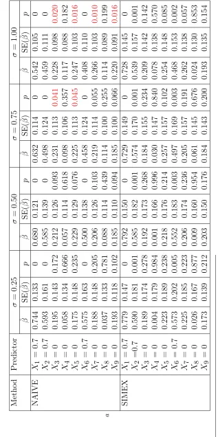
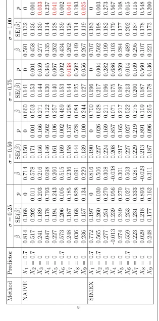
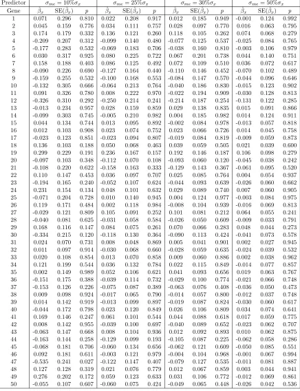
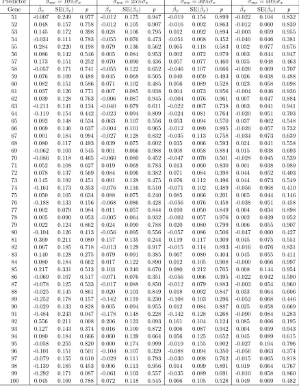
Using the naive and SIMEX methods, Tables 2.1 and 2.2 report the results of
the parameter estimates,βb, its standard errors, SE(βb), which is computed using 1000
bootstraps and the corresponding p-values under different degrees of measurement
error and α = 1.5. Tables 2.5 and 2.6 reports the results of the same settings but
α = 0.5. Since the gene expressions from the microarray may be correlated with
each other, we assume that the genes have been rearranged based on their functional
similarity. We generated gene expressions using the exchangeable covariance matrix,
where gene expressions are only correlated with the ones right beside them. Tables
2.3 and 2.4 contain the results of using the exchangeable covariance matrix.
When the measurement error is minor (i.e., σ = 0.25) or moderate (i.e., σ =
0.50), the impact of measurement error is not noticeable. The naive method, which
Xπ(i) replaced byWπ(i), can select the true model. However, when the measurement
error becomes increasingly larger, the effect of measurement error is more obvious.
The bias of theβb increases, while the SE(βb) decreases. The covariates,Xi1,Xi2 and
Xi6, which should be in the true model, can be selected. However, as the measurement
error becomes severe, those covariates that are not actually in the true model were
improperly selected since their p-values were typically smaller than the 5% level.
Afterwards, the SIMEX approach was employed with B = 50, λM = 2 and
M = 11 to adjust the impact of measurement error to the selection of variables. In
this chapter, we choose to use quadratic extrapolation for the SIMEX method as
used in He et al. (2007). The results are listed in Tables 2.1 to 2.4. These results
show that the SIMEX approach improves the performance of variable selection when
measurement errors are present. The SIMEX method gives good estimates of βx,
especially those that are not present in the true model, since the biases are smaller
and thep-values provide the correct conclusion at the 5% significance level. However,
when the measurement error is severe, the SIMEX method seems to perform less
satisfactorily. The bias tends to increase as the degree of measurement error increases.
By comparing the estimates reported in Tables 2.1 to 2.6, we find that the proportion
of censoring could also affect the estimation of βx since the censoring rate is highly
2.4
Real Data Analysis
2.4.1 PBC Data
The PBC data were collected from the Mayo Clinic trial conducted between 1974 and
1984. A wide range of health-related covariates were collected for 312 randomized
participants. See Tibshirani (1997) for the detailed description of those covariates.
We first transform the survival time and some covariates on 276 complete observations
of the PBC data according to the recommendations by Huang et al (2006). These 276
patients were followed from diagnosis until death or censoring, where the censoring
rate was 59.78%. We fit both the AFT model with the Weibull distribution and AFT
model by regularizing IPW estimate with adaptive LASSO penalty on these data.
Standard error estimates are obtained by using the bootstrap with 1000 replications.
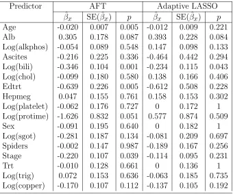
Table 2.7 provides the results for the estimate, the standard error and the p
-value for all covariates used in both methods. It seems that the AFT model using
the adaptive LASSO regularized IPW method yields a smaller model than the AFT
model using the Weibull distribution. Therefore, we will use only the adaptive LASSO
regularized IPW method for the investigation of the impact of the measurement error.
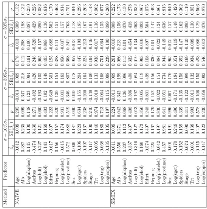
We conduct sensitivity analysis by adding different levels of measurement error
to the covariates to assess the impact of measurement error on variable selection
in the PBC data. Measurement errors are randomly and independently added to
the continuous covariates. They are generated from N(0, σ2), where the standard
deviation, σ, is proportional to the standard deviation, σx, of the corresponding
covariate. The proportions are set to be 10%, 30% and 50% to represent various
degrees of measurement error.
Table 2.8 shows the results of the estimate, associated standard error and
corre-sponding p-value from the sensitivity analysis. The error free covariates do not seem
to be greatly affected by the error prone covariates. In the naive method, as
estimate decreases. The impact of measurement error on estimation of the log(bili) is
very noticeable. For the original PBC data, the adaptive LASSO regularized IPWp
-value of log(bili) in Table 2.7 is 0.043 (i.e., log(bili) is significantly associated with the
survival time). The naive method computes p-values greater than 5% under different
degrees of measurement error; this concludes that there is no evidence that log(bili)
is a survival related covariate, which conflicts with the result from the original data.
On the other hand, the SIMEX method makes adjustment to the effect of
measure-ment error. The estimates from the SIMEX method have smaller bias compared to
the naive method. The correspondingp-values are more consistent with the p-values
given by the adaptive LASSO method of the original PBC data set.
Table 2.7: Fit the AFT model to PBC data using adaptive LASSO regularzied IPW method. ˆβx: estimate of coefficient; SE( ˆβx): the bootstrap standard error; p: the
corresponding p-value.
Predictor AFT Adaptive LASSO
ˆ
βx SE( ˆβx) p βˆx SE( ˆβx) p
Age -0.020 0.007 0.005 -0.012 0.009 0.221
Alb 0.305 0.178 0.087 0.393 0.228 0.084
Log(alkphos) -0.054 0.089 0.548 0.147 0.098 0.133
Ascites -0.216 0.225 0.336 -0.464 0.442 0.294
Log(bili) -0.346 0.104 0.001 -0.234 0.115 0.043 Log(chol) -0.099 0.180 0.580 0.138 0.166 0.406
Edtrt -0.639 0.226 0.005 -0.612 0.508 0.228
Hepmeg 0.047 0.155 0.761 0.158 0.153 0.302
Log(platelet) -0.062 0.176 0.727 0 0.172 1
Log(protime) -1.626 0.832 0.051 0.577 0.874 0.509
Sex -0.091 0.195 0.640 0 0.182 1
Log(sgot) -0.281 0.187 0.134 -0.081 0.209 0.697
Spiders -0.002 0.147 0.987 -0.189 0.167 0.256
Stage -0.220 0.107 0.039 -0.114 0.095 0.231
Trt -0.010 0.128 0.661 0 0.136 1
T able 2.8: PBC data: Sensitivit y analysis with all of the quan titativ e co v ariates sub jec t to measuremen t error Metho d Predictor σ = 10% σx σ = 30% σx σ = 50% σx
ˆβx
SE(
ˆβ)x
p
ˆβx
SE(
ˆβx
)
p
ˆβx
SE(
ˆβx