Schmid, Karl (2009): Supersonic Micro-Jets And Their Application to Few-Cycle Laser-Driven Electron Acceleration. Dissertation, LMU München: Fakultät für Physik

(1)

Supersonic Micro-Jets

And Their Application to

Few-Cycle Laser-Driven

Electron Acceleration

Karl Schmid

(2)

(3)

Supersonic Micro-Jets

And Their Application to

Few-Cycle Laser-Driven

Electron Acceleration

Karl Schmid

Dissertation

an der Fakultät für Physik

der Ludwig–Maximilians–Universität

München

vorgelegt von

Karl Schmid

aus Wien

(4)

(5)

List of Figures

1 Electron acceleration in the bubble regime . . . 5

2 Threshold of the Bubble Regime . . . 7

3 Sketch of a typical de Laval nozzle . . . 10

1.1 Rankine-Hugoniot curve for the perfect gas . . . 21

1.2 Shock in a perfect gas . . . 24

1.3 Normalized flow density within a de Laval nozzle . . . 27

1.4 Flow parameters inside a de Laval nozzle - 1D model . . . 28

1.5 Flow state at the exit of a de Laval nozzle . . . 31

1.6 Clustering in Ar and He jets . . . 33

2.1 Parameterization of de Laval Nozzles . . . 37

2.2 Knudsen number for different pressures . . . 37

2.3 Line-outs normal to flow direction inside a de Laval nozzle . . . 39

2.4 On-axis line-outs inside a de Laval nozzle . . . 41

2.5 Divergence of gas jets produced by subsonic and supersonic nozzles . . . 42

2.6 Density profiles of gas jets produced by subsonic and supersonic nozzles . 43 2.8 Geometry study: free jet propagation . . . 49

2.9 Geometry study: displacement thickness . . . 50

2.10 Geometry study: gradient width . . . 53

2.11 Geometry study: density gradient width. Linear dependence onL×dC/dE 54 2.12 Geometry study: flat top quality . . . 54

2.13 Geometry study: density peak-to-peak fluctuations . . . 55

2.14 Pressure and size study: Knudsen numbers of pressure and size series . . 56

2.15 Pressure and size study: gas jet divergence . . . 57

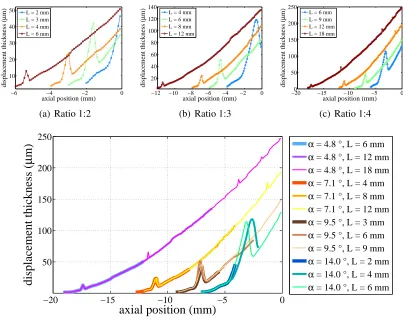
2.16 Pressure and size study: flow displacement . . . 58

2.17 Pressure and size study: displacement thickness at nozzle exit . . . 59

2.18 Pressure and size study: density gradient width . . . 60

(10)

x LIST OF FIGURES

2.20 Pressure and size study: density and Mach number at nozzle exit . . . 61

2.21 Pressure and size study: exit density vs. backing pressure for different nozzle sizes. . . 61

2.22 Pressure and size study: density peak-to-peak fluctuations . . . 63

2.23 Influence of background pressure . . . 65

2.24 Double nozzle . . . 66

2.25 Shock fronts produced by knife-edge in the supersonic gas jet. . . 67

3.1 Mach-Zehnder interferometer . . . 70

3.2 Abel inversion sketch . . . 71

3.3 Gas jet characterization for 150µm nozzle . . . 73

3.4 Measured on axis density and stability . . . 75

3.5 Supersonic shock front measurement . . . 77

4.1 Artist’s conception of a plasma bubble . . . 96

4.2 PIC simulation: physical state of plasma . . . 101

4.3 PIC Simulation: Electron Spectrum . . . 103

5.1 Layout of LWS-10 . . . 106

5.2 Measured pulse duration and focal spot of LWS-10 . . . 108

5.3 Peak-to-background contrast of LWS-10 . . . 109

5.4 Photograph of the Experimental Chamber . . . 110

5.5 Experimental layout of electron accelerator . . . 111

5.6 Simulated magnetic field map of electron spectrometer . . . 113

6.1 Low background energy spectra . . . 117

6.2 Typical electron spectrum (Lanex) . . . 119

6.3 Electron energy fluctuation . . . 121

6.4 Density and spot size variation . . . 122

6.5 Gas jet position scan . . . 124

6.6 Shot series of 27 monoenergetic electron spectra . . . 125

6.7 Reproducible electron spectra with 150µm gas jet . . . 126

6.8 Electron spectrum showing multiple bunches . . . 126

6.9 High energy electron spectra showing multiple bunches . . . 127

7.1 Wake field at density transition . . . 133

7.2 Ratio between plasma wave period and mean free path . . . 136

A.1 Shock fronts in a nozzle with smaller radii . . . 144

(11)

List of Figures xi

A.3 Comparison of turbulence models: density contours . . . 150

A.4 Comparison of turbulence models: boundary layer . . . 151

B.1 Nozzle design with 150µm exit diameter . . . 154

B.5 Nozzle design with 1 mm exit diameter . . . 158

B.6 Nozzle design with 1.5 mm exit diameter . . . 159

(12)

(13)

List of Tables

1.1 Flow parameters in a de Laval nozzle with air . . . 29

1.2 Flow parameters in a de Laval nozzle with helium . . . 30

2.1 Flow regimes according to Knudsen number . . . 38

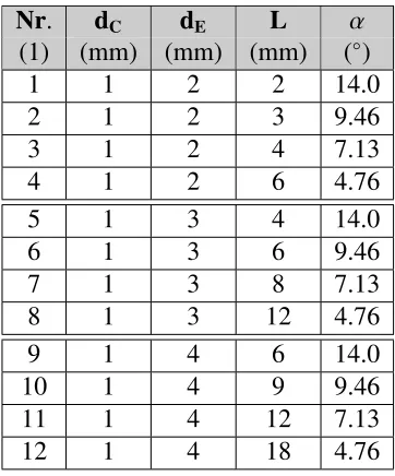
2.2 Parameter study: nozzle geometry - list of simulations . . . 47

2.3 Parameter study: nozzle size and pressure - power law fits. . . 62

2.4 Parameter study: nozzle size and pressure - list of simulations. . . 64

3.1 Refractive index of several gases . . . 70

(14)

(15)

Zusammenfassung

Diese Doktorarbeit handelt von der durch ein Plasma vermittelten Beschleunigung von Elektronen durch ultrakurze Lichtpulse. Diese sogenannteLaser Wakefield Accelerationist ein lange bekanntes Konzept, welches auf der Ausnutzung von lasererregten Plasmawellen großer Amplitude zur Erzeugung von Be-schleunigungsgradienten im Bereich von mehreren 100 GV/m beruht. Dieser Wert ist um etwa vier Grö-ßenordnungen höher als der durch den beginnenden elektrischen Durchschlag im Vakuum festgelegte Maximalwert, der mit klassischen Beschleunigern erreicht werden kann und der etwa 100 MV/m nicht überschreitet. Diese drastische Erhöhung der Beschleunigungsfelder erlaubt eine ebenso signifikante Re-duktion der Beschleunigungstrecke, die zum Erreichen einer bestimmten Energie erforderlich ist. Ein auf diesem Prinzip beruhender Teilchenbeschleuniger wäre daher um Größenordungen kleiner und ko-stengünstiger als ein klassischer Beschleuniger mit ähnlicher Leistung. Zusätzlich eröffnen die speziellen Eigenschaften der laserbeschleunigten Elektronenpulse in Gestalt von ultrakurzer Pulsdauer, hoher Bril-lanz sowie hoher Ladungsdichte gänzlich neue Horizonte.

Das in dieser Arbeit verwendete Lasersystem ist eine Neuentwicklung und beruht auf optischer pa-rametrischer Lichtverstärkung. Dieser spezielle Lichtverstärkungsprozess ermöglicht die Verstärkung ul-trakurzer Lichtpulse mit einer Pulsdauer von nur 8 fs auf eine Leistung von 6.5 TW. Dies ist weltweit einzigartig. Der Laserstrahl wird im Experiment auf einen Heliumjet fokussiert, was zur sofortigen Bil-dung eines Plasmakanales führt, durch den die Lichtpulse propagieren. In der hochgradig nichtlinearen Wechselwirkung zwischen dem Lichtfeld mit Intensitäten im Bereich von 1019_W/_cm2 _{und dem Plasma}

mit einer Elektronendichte von 2×1019cm−3entsteht eine stark anharmonische Plasmawelle. Die Ampli-tude dieser Welle ist hierbei so hoch, dass die Welle bricht und Elektronen aus dem Hintergrundplasma von der Plasmawelle beschleunigt werden.

Der Energietransfer vom Laserpuls zu der von ihm getriebenen Plasmawelle ist so stark, dass die maximale Propagationslänge im Bereich von 100 µm liegt. Daher ist es notwendig, speziell auf die-se Anforderungen abgestimmte Gasjets zu benützen. Das Verhalten von überschallschnellen Gasjets im Größenbereich von 100µm wird deshalb im Rahmen dieser Arbeit ausführlich analysiert. Diese haupt-sächlich auf numerischer Strömungssimulation beruhende Analyse umfaßt mehrere umfangreiche Para-meterstudien, die alle relevanten Aspekte mikroskopischer Überschallströmungen beleuchten, was in der Folge das optimierte Design und die Herstellung von Lavaldüsen zur Erzeugung von überschallschnel-len Gasjets in einem Durchmesserbereich von 150 µm - 3 mm erlaubte. Der Einsatz dieser Düsen im Experiment führte zu einer signifikanten Verbesserung der Stabilität des Elektronenstrahls und zu einer hervorragenden Übereinstimmung von Simulation und Experiment.

(16)

Abstract

This thesis covers the few-cycle laser-driven acceleration of electrons in a laser-generated plasma. The so-calledlaser wakefield accelerationis a long-known concept that relies on strongly driven plasma waves for the generation of accelerating gradients in the range of several 100 GV/m. This value is approximately four orders of magnitude larger than the one attainably by classic accelerators, which is limited essentially by electrical breakdown in the accelerating structures to approximately 100 MV/m. Since the acceleration length necessary for obtaining a certain electron energy is inversely proportional to the accelerating field, this leads also to a drastic reduction of the size and of the price of the accelerator. Furthermore, the special properties of laser accelerated electron pulses, namely the ultrashort pulse duration, the high brilliance, and the high charge density, open up new possibilities in many applications of these electron beams.

The laser system employed in this work is a new development based on optical parametric chirped pulse amplification and is the only multi-TW few-cycle laser in the world. It allows for the amplification of pulses with a duration of 8 fs up to a power of 6.5 TW. In the experiment, the laser beam is focused onto a supersonic helium gas jet which leads to the formation of a plasma channel. The laser pulse, having an intensity of 1019 _W/_cm2 _{propagates through the plasma with an electron density of 2}_×₁₀19

cm−3_{and forms via a highly nonlinear interaction a strongly anharmonic plasma wave. The amplitude of}

the wave is so large that the wave breaks, thereby injecting electrons from the background plasma into the accelerating phase.

The energy transfer from the laser pulse to the plasma is so strong that the maximum propagation distance is limited to the 100 µm range. Therefore, gas jets specifically tuned to these requirements have to be employed. The properties of microscopic supersonic gas jets are thoroughly analyzed in this work. Based on numeric flow simulation, this study encompasses several extensive parameter studies that illuminate all relevant features of supersonic flows in microscopic gas nozzles. This allowed the optimized design of de Laval nozzles with exit diameters ranging from 150µm to 3 mm. The employment of these nozzles in the experiment greatly improved the electron beam quality.

(17)

Introduction

Motivation

For a century, the on-going development of particle accelerators has been promoting many branches of fundamental and applied research. What began as a tool for nuclear and par-ticle physics, has expanded its use into solid state physics as well as medicine, biology and even history [1]. As these lines are written, the superconducting magnets of the Large Hadron Collider (LHC) [2] – [8] at the CERN laboratory are being cooled down to liquid Helium temperature and in a few months’ time, the largest collider ever built will com-mence operation. With its two counter-propagating proton beams having 7 TeV energy each, it is expected to shed new light on hot topics such as the fundamental origin of mass in form of the famous HIGGS Boson [9], dark energy and dark matter [10], the possible existence of small extra dimensions in space-time [11], and many more. However, looking at the tremendous scale of this project, it is valid to ask the question whether this collider will actually staythe largest collider ever built for many decades to come. With the Su-perconducting Super Collider (SSC) [12] – [15] in Texas, USA, having been cancelled in 1993 due to exploding cost-forecasts that saw the final price tag exceeding 12 billion USD, the only remaining accelerator project which is of comparable magnitude to the LHC is the International Linear Collider (ILC) [16], [17]. The latter will - if realized - consist of two linear accelerators, in head-on configuration, one accelerating electrons, the other one positrons. The entire structure will stretch over a length of 31 km and will be able to reach a particle energy of 500 GeV in each beam. With a projected total cost of 5 billion USD, it can only be realized by an international collaboration of several contributing countries.

(18)

2 Introduction

radiation losses in synchrotron configuration [19], the accelerator needs to be more than 30 km long.

This is where plasma based electron accelerators offer great advantages due to their orders of magnitude larger accelerating gradients which in turn allow for much shorter acceleration length. In this accelerator concept a laser- or ultra-relativistic electron pulse is used to excite a plasma wave which then serves as accelerating structure. As the pulse propagates through the plasma, it excites a running, longitudinal charge separation wave -called Langmuir wave - that trails the electron or laser pulse and, therefore, has a phase ve-locity equal to the group veve-locity of the laser pulse or equal to the veve-locity of the electron pulse. Depending on plasma density and electron temperature, this type of wave generates longitudinal electric fields in the 1 GV/m to 1 TV/m range. This concept of using a travel-ling plasma wave as an accelerating structure was first presented by Tajima and Dawson in 1979 when they proposed to excite such a plasma wave by means of a short and powerful laser pulse [20].

Plasma-Based Electron Acceleration - A Historical Overview

With the prospects of this new concept as a motivation, diverse schemes to excite longitu-dinal plasma waves and to use them for electron acceleration were experimentally investi-gated, the most important ones being the plasma wakefield accelerator (PWFA) [21] – [26], the plasma beatwave accelerator (PBWA) [27] – [31], and the laser wakefield accelerator LWFA [32] – [47].

In the case of PWFA, the plasma wave is excited by one or more relativistic electron bunches and another pre-accelerated bunch is then injected and accelerated by the plasma wave. For many years, maximum energy gains were quite moderate in this field [21] - [24] with a maximum gain of 30 MeV of an electron bunch with an initial energy of 500 MeV [23]. A more complete account of the developments in this field up to the year 1995 can be found in [48]. When improving electron bunch parameters allowed better matching of electron bunch size and length to the plasma density, substantial energy gain in the GeV range was demonstrated [25] and the so-called plasma-afterburner was recently shown to be capable of energy-doubling the trailing edge of a short and dense 42 GeV electron bunch in a meter-scale plasma [26].

(19)

Introduction 3

electrons [27]-[31]. Energy gains up to 28 MeV have been shown in this scheme [28], [29].

As powerful ultrashort pulse lasers became available, the initial concept of laser wake-field acceleration could be realized. In LWFA, a short (τ <1ps), ultra-intense (I > 1018 W/cm2) laser pulse drives the plasma wave. The plasma wave excitation is most efficient, when the laser pulse length is approximately equal to or shorter than the plasma wave-length. The first experimental evidence of the excitation of a plasma wave in the LWFA regime was found in 1993 by Hamster et al. [32] and two years later also by other groups [34], [35]. In 1995, electron acceleration by LWFA was shown by injecting electrons emit-ted from a laser-solid interaction into a low-density plasma wave by Nakajima et al. [33]. In this case, an 8 TW, 1 ps laser pulse impinged on a plasma with a density of 3.5×1015 cm−3 _{thereby exiting a plasma wave that accelerated the injected electrons from an}

ini-tial energy of 1 MeV to a final one of 8 MeV corresponding to an estimated accelerating gradient of 0.7 GV/m.

As mentioned previously, in principle much larger accelerating fields are feasible but they require the plasma wave to be driven much stronger than it was possible in the early days of CPA by a single pulse that was resonant with the plasma wave. Therefore, the self-modulated laser wakefield (SM-LWFA) scheme was proposed [50] – [52]. As the standard LWFA, the driving laser pulse has a sub-ps duration and an intensity typically larger than 1018_W_/_cm2_{but the plasma density is larger here such that the laser pulse length is (much)}

longer than the plasma wavelength. The plasma density is typically chosen such that the laser pulse power is a little bit larger than the critical power for relativistic self-focusing [53] – [57]. In this case, self guiding occurs which compensates diffraction and, there-fore, causes the laser pulse to maintain or surpass its focal intensity for a distance that can greatly exceed the Rayleigh-range of the beam. The Rayleigh-range is the on-axis distance from the laser focus where the laser intensity is reduced to half its value in the focal spot due to diffraction. This prolonged interaction with the plasma at ultrahigh in-tensity allows for the growth of the self-modulation or beam-breakup instability which splits the laser pulse up into multiple beamlets each of which then drives the plasma wave resonantly. In this way, highly anharmonic Langmuir waves can be excited leading to enhanced acceleration gradients. The beam-breakup can be described in terms of the for-ward Raman-scattering instability [58], [59] where the strong electromagnetic pump wave (ω, k) decays into a plasma wave (ωp, kp) and two forward-propagating electromagnetic

waves at the so-called Stokes (ω−nωp) and anti-Stokes (ω+nωp) frequencies. Herenis an

(20)

4 Introduction

First experimental evidence for wake field excitation in this regime was presented by Coverdale et al. in 1995 [40]. Again, Nakajima et al. were the first to show acceleration in this regime in the same year [41] by injecting and accelerating a 1 MeV electron bunch up to 17 MeV with an estimated acceleration gradient of 30 GV/m. They used a 3 TW, 1 ps, 1017W/cm2 pulse in a plasma with an electron density of 1019 cm−3. Subsequently, electron acceleration in the SMLWFA regime was realized in many experiments [42] -[46]. Modena et al. were the first to show substantial wave breaking in the self modulated regime which was accompanied by clearly non-maxwellian spectra with maximum ener-gies around 44 MeV. Gahn et al. [60] showed that in the laser and plasma parameter region of SM-LWFA, a competing electron acceleration process termed direct laser acceleration (DLA) exists which under certain circumstances dominates over wakefield acceleration. The largest electron energy in SM-LWFA as well as in the DLA regime so far was shown in 2005 by Mangles et al. using a petawatt laser where exponentially decaying energy spectra and spectra following a power law with a maximum energy larger than 300 MeV were shown. Common to all the above mentioned experiments is the large electron energy spread that makes the generated electron beams of limited use for application.

Meanwhile, with continuing laser development, Ti:sapphire based CPA lasers reached ever shorter pulse durations with increasing pulse energies. Eventually this allowed exper-imenters to go back to the initial LWFA concept as the short pulse durations now allowed the use of a pulse short enough to fit into one plasma wavelength and still drive the wave strong enough to reach wave breaking. On the border between LWFA and SM-LWFA, some authors, such as Malka et al. in 2002, speak of the "forced-LWFA"-regime [47] where these new ultrashort (∼40 fs) and relativistically intense (> 1018W/cm2) pulses are used in plasmas with a density around 1019 _cm−3 _{so that still several plasma wavelength}

fit into the laser pulse. While this regime produced pedestal-type spectra that were clearly non-maxwellian [47] it fails to produce monoenergetic spectra that are demanded by most applications.

(21)

Introduction 5

Figure 1: Particle-In-Cell (PIC) simulation of electron acceleration in the bubble regime with 40 mJ, 8.5 fs (FWHM) laser pulses. (a) shows the physical state (plasma density, grey-scale contour, instantaneous laser intensity, rainbow contours and longitudinal electric field, red line) of the

accel-erator after 123µm propagation. (b) is the electron energy spectrum after the accelerated electron

bunch propagated out of the plasma. Simulations courtesy of Michael Geissler [61].

the laser pulse is so large that the majority of the free electrons are transversally pushed out leaving the positively charged ions behind. After a propagation length comparable to a plasma wavelength, the electrons are driven back to the axis by the fields built up by charge separation. A cavity void of electrons trailing the laser pulse emerges: it has been dubbed a "bubble" [62]. A fraction of the returning electrons is injected and trapped in the bubble and accelerated by its strong longitudinal electric field resulting in relativistic electron bunches with narrow-band energy spectra [65], [66].

Only recently laser pulses with parameters coming close to the requirements of the bubble regime - like in the present work and in Hafz et al. [67] - became available, so it came as a surprise when in 2004 three independent groups showed the generation of monoenergetic electron beams, namely Faure et al. [68], Geddes et al. [69], and Mangles et al. [70]. In all the three cases the employed laser pulses did not initially match the re-quirements prescribed by the so-called "Bubble-Regime" by Pukhov and Meyer-ter-Vehn. PIC simulations conducted with the exact experimental parameters [68] – [70] showed that self-focusing and self-compression of the laser pulses in the plasma finally transformed the pulses into the required domain.

(22)

6 Introduction

by Hidding et al. [71] - work in the above described regime where the laser pulse initially (almost) fits into one plasma wavelength but only through some self-modulation acquires high enough intensity to drive the wake wave into breaking. Leemans et al. demonstrated the record electron energy of 1 GeV [72], using a discharge in a gas-filled capillary to guide the 40 fs, 40 TW laser pulse with an initial intensity of 3×1019 W/cm2 over a cm-scale distance in a 3×1018_cm−3_{plasma and, thereby, maximizing the acceleration length.}

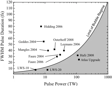
Faure et al. [73] showed that by using a second weaker, counter-propagating laser pulse that was overlapped with the primary driver pulse in a 7.5×1018cm−3plasma injection of background electrons into the plasma wave could be triggered without actually driving the plasma wave to breaking. This leads to a greatly improved shot-to-shot reproducibility of the monoenergetic electron beam and also allows tuning of the injected charge and elec-tron energy [74]. Both laser pulses had 30 fs duration, the driving laser with 24 TW power and the injection laser with 8.3 TW. Osterhoff et. al [75] showed improved shot-to-shot reproducibility by employing a steady-state gas-cell as a target and Hafz et al. [67] also showed improved stability by using ultra-high power (110 TW) ultrashort (32 fs) laser pulses. As a summary to the LWFA experiments that generated monoenergetic electron pulses, figure 2 shows the relation of pulse duration versus pulse power of the above cited experiments together with the threshold that defines the bubble regime. Here, the grey area is within and the white area is outside this regime. The figure clearly shows that the present work is together with Hafz et al. the only one that falls into this regime and that it is far removed from all other experiments thereby exploring an entirely new parameter range.

The Present Electron Acceleration Work

(23)

Introduction 7

1 10 100 1000

10 20 30 40 50 60 70 80 90 100 110 120 Atlas Upgrade LWS-20 Osterhoff 2008 Faure 2006 Leemans 2006 Faure 2004 Geddes 2004 Mangles 2004 F W H M P u l s e D u r a t i o n ( f s )

Pulse Power (TW)

LWS-10 Hafz 2008 Hidding 2006 L i m it o f B u b b l e R e g i m e

Figure 2: Pulse duration limit (fs) of the bubble regime vs. pulse power (TW) (solid line). The allowed parameter range for the bubble regime is shaded in grey. Parameters of former and present experiments (black rectangles). The following experiments are included: Mangles 2004 [70], Ged-des 2004 [69], Malka 2004 [68], Leemans 2006 [72], Faure 2006 [73], Hidding 2006 [71],

Os-terhoff2008 [75], Hafz 2008 [67]. LWS-10 corresponds to the present work and LWS-20 to the

parameter of an upgrade of the system that is under way. "Atlas Upgrade" corresponds to the planned parameters of the upgraded Ti:sapphire laser system ATLAS at the Max-Planck-Institute of Quantum Optics.

Motivation for the development of microscopic de Laval nozzles

(24)

8 Introduction

Supersonic (Micro) Gas Jets

A central problem in laser-plasma physics is posed by the fact that high power lasers, with laser pulse powers typically larger than 1 TW, cannot be focused in air or any other am-bient medium without being strongly modified by ionization of and subsequent nonlinear interactions with the medium leading to strong spatial and temporal pulse modulation and beam breakup. Therefore, in order to reach the intensities of more than 1018_W/_cm2_typical

in such experiments, the laser must be brought to its focus in an evacuated chamber. In order to obtain clean interaction conditions, a gas target is needed that is spatially well confined so that interaction happens only at the ultrahigh intensity laser focal spot. Sev-eral different methods are used in this context in order to obtain gas densities that typically lie between 1018 and 1020 1/cm3. The easiest way would certainly be a simple gas filled chamber with windows for the laser but of course this cannot be used because the win-dows would immediately be destroyed by the laser. Therefore, either gas jets that emanate into the vacuum or gas cells with holes allowing the laser to pass through or gas filled capillaries with open ends have to be used. All of these methods have in common that a substantial gas load is produced which has to be supported by the vacuum pump system. Many laser-plasma interactions are strongly nonlinear processes and plasma parametric instabilities make the interaction dynamics depend strongly on the exact density profile of any given target and on its shot-to-shot reproducibility. This makes tailored and well characterized gas targets an essential prerequisite for these experiments.

Supersonic gas jets represent a unique tool to produce reproducible, spatially well confined gas targets which offer the possibility of producing flat-top density profiles and steep gradients at the jet edges. Therefore, they are employed in a great number of laser-plasma experiments. The types of experiments are manyfold, a recently very popular one is laser driven electron acceleration [48], [67] – [71] , [73], [77] – [85]. Others include generation of THz [86] – [88], X-UV [89] and X-ray [90] – [94] beams as well as ion beams [95], [96], and laser pulse compression [97] or laser frequency upshift [98] and the generation of strong, quasistatic magnetic fields [99], [100].

(25)

Introduction 9

diffraction [110], nuclear scattering [111], stimulated Raman scattering [112], white light generation [113], linear Raman spectroscopy [114], and, most frequently used for high density jets, interferometrically [115] – [120]. These studies present measurements for a small number of nozzle designs used in the experiments. Some authors published work on the optimization of a specific nozzle design via numeric flow simulation [121], [122]. To the authors’ knowledge, only one work exists representing first steps towards the sys-tematic numeric and experimental optimization of the properties of mm-size supersonic gas jets close to the nozzle exit for laser-plasma experiments [121]. No study exist so far on the specific behavior of supersonic flows inside microscopic nozzles in the context of laser-plasma physics.

Part I of this work reports on the systematic simulation, design, and characterization of supersonic gas jet targets for electron acceleration with ultra-high intensity ultra-short pulse lasers. As detailed above, the laser-parameters at hand dictate the use of very small gas jet diameters in the 100 µm range. At the same time, the fact that the laser focal spot can, depending on focusing conditions, be in the range of tens of micrometers causes the additional requirement that the gas jet should stay collimated and sharp-edged and maintain its flat top profile over a distance of up to one nozzle exit diameter. It will be shown that supersonic gas jets from correctly designed de Laval nozzles fulfill all these requirements in a wide parameter range in terms of gas density and nozzle size. A sketch of such a nozzle is depicted in Figure 3.

The feasibility of microscopic supersonic jets has so far mainly been investigated in the context of micro-thrusters for small scale spacecraft, simulations being done mostly in 2D owing to the geometry of those thrusters [123], [124]. In this context, many publications exist on comparison and benchmarking of different flow models for rarefied flows [125] – [132], on the optimization of thrusters for microelectromechanical systems (MEMS) [133] – [136], on properties of jets emanating into surrounding atmosphere [137] and on the fabrication of de Laval micronozzles [138]. The main goal in these publications is to maximize the efficiency and hence the thrust per mass unit of propellant and not the flow profile after the nozzle exit.

(26)

10 Introduction

Figure 3: Sketch of a converging-diverging de Laval nozzle as it was used in the present simulations

and experiments. On the left side, the nozzle is attached to a gas reservoir with a pressure p0 of

typically between 10 and 100 bar and with a temperature T0 of 300 K. The gas is allowed to

expand through the nozzle into an evacuated chamber. In the diverging section of the nozzle after the nozzle throat supersonic conditions are reached. The arrow indicates the direction of the gas flow. The supersonic jet emanating into the vacuum has low divergence, a flat top density profile and sharp edges. This is shown in the sketched density profile showing a line-out of the gas density

ρperpendicular to the jet axis versus the jet radius r.

Structure of the Thesis

The present work is structured in two parts:

Part I, containing chapters 1 through 3, is devoted to an in-depth study of supersonic gas flows in microscopic nozzles:

chapter one summarizes the most important and relevant parts of the theory of compress-ible fluid flow. It starts with basic concepts, such as the equation of state and different types of state changes, then introduces several effects like shock front formation and propagation of distortions at supersonic speed which are peculiar in supersonic gas flows. Cluster formation in supersonic gas flows is also covered in so far as it is relevant to the present work.

(27)

Introduction 11

chapter three presents experimental results about the characterization of microscopic su-personic gas jets. It is shown that simulation and measurement agree well and that supersonic gas jets with diameters as small as 150 µm can be produced by micro-scopic de Laval nozzles. It also shows the first experimental steps towards gas targets with structured density profiles.

Part II, spanning chapters 4 through 7, covers electron acceleration in relativistic plasma waves driven by few-cycle laser pulses:

chapter four summarizes the analytical and simulation results that are relevant for laser-driven electron acceleration. This includes important effects in analytical description as wake field formation, relativistic self-focusing of laser-pulses, and wave breaking. Empirical laws derived from particle-in-cell (PIC) simulations are discussed as well as the results of PIC simulations matching the experimental conditions in the present laser driven accelerator.

chapter five contains a description of the experimental setup, covering the light-source and the actual electron accelerator.

chapter six gives an account of the main experimental results obtained in the course of this work. The typical electron beam parameters are summarized and results con-cerning stability and tunability of the acceleration process are presented. A detailed discussion of the experimental results is given.

chapter seven discusses the most important problems that need to be solved in the future and presents several promising routes towards the solution of these problems.

(28)

(29)

Part I

(30)

(31)

Chapter 1 Theory of Compressible Fluid Flow

1.1 One Dimensional Theory of Compressible Fluid Flow

1.1.1 Equation of State and the First Principal Law

The thermodynamic properties of a homogeneous and isotropic medium are fully charac-terized by the three quantitiestemperature T (K),pressure p(Pa), and densityρ(kg/m3) which are called the state variables. About the microscopic structure of the medium the only necessary assumptions are that the particles that constitute the medium are small enough to justify the assumption of homogeneity and that for any given set ofT, p,ρthe composition of the medium is fixed. This includes, for example, mixtures of gases or air that contains a certain amount of water in the form of small droplets.

The quantitiesT, p, ρdepend on each other, their relation is given by the equation of state of that medium.

p= p(ρ,T) (1.1)

Additional state variables can and will be defined and used but - together with the equation of state - always two of them are enough to characterize the state of the medium. In the case of a perfect gas the equation of state has the well known form

p= R

mρT (1.2)

whereRis the gas constant that is given byR= kBNA = 8314.46 J/(kgK). HerekB is the

Bolzmann constant andNA the Avogadro constant. mis the atomic (molecular) weight of

the medium.

(32)

16 1. Theory of Compressible Fluid Flow

The quantity that measures the energy content of a medium is the inner energy e and is a state variable on its own. Hence, it only depends on two other state variables, for ex-ample, e = e(p, ρ) which again represents an equation of state. In the case of the perfect gas, the inner energy only depends on the temperature e = e(T). This inner energy is constant as long as the gas is not doing any work thereby converting a part of its inner energy into mechanical energy. This does not entirely exclude changes of the volume of the gas as can be seen in the following case: a perfectly isolated vessel that is separated in two compartments by a removable wall with one compartment being filled with a gas of a certain pressure and temperature. By removing the wall, the gas will now expand and fill the entire vessel. Since there is now energy (heat) transport through the vessel walls, the inner energy must be conserved which means for a perfect gas that after the expansion is completed the gas will still have the initial temperature. This is a so-called irreversible adi-abatic expansion because it is impossible to reach the initial state without energy transfer to the gas. If the wall is now replaced by a slowly moving piston, the situation is different: the gas exerts a force on the piston corresponding to its pressure times the piston surface. By moving the piston a distance ds, the work pAds is done. Since Ads is equal to the change of the volume of the gas, the amount of work done is given by pdV = pd(1/ρ). If heat transport to the medium dq is now considered, then the law of energy conservation takes on the form:

dq= de+ p d(1/ρ) (1.3)

Here the amount of heat q is measured in joule per kg. This equation is called the first principle law of thermodynamics. With the enthalpyibeing defined as

i=e+ p/ρ (1.4)

it can be written as

dq= di−1/ρdp (1.5)

Heat can be transferred to a medium in different ways, the two most easily realizable methods are maintaining the volume and hence the density constant and keeping the pres-sure constant. By measuring the amount of energy needed to raise the temperature of the medium by 1 K one arrives at the definition of the specific heatscpandcv. They are defined

as

cv = _∂∂q

T

!

v = _∂∂e

T

!

v

(1.6)

for constant volume and as

cp =

∂q ∂T

!

p

= _∂∂i

T

!

p

(33)

1.1 One Dimensional Theory of Compressible Fluid Flow 17

for constant pressure. The ratio between the specific heat is ascribed the symbolκand is defined as

κ=cp/cv κ=

2+ f

f (1.8)

The equation to the right gives a connection to the kinetic theory of gases with f corre-sponding to the number of degrees of freedom of the molecules constituting the medium. Possible values for f are therefore 3 for atoms, 5 for molecules containing 2 atoms and 7 for molecules containing three or more atoms.

For the perfect gas, one obtains for the specific heats

de=cvdT (1.9)

and

di= cpdT (1.10)

Substituting this into (1.4) and using (1.2) we get

R/m= cp−cv (1.11)

With the additional assumption that a medium not only behaves like a perfect gas but also has constant specific heatscpandcvfor all temperatures from (1.9) and (1.10) we get

e=cvT +const (1.12)

and

i= cpT +const (1.13)

1.1.2 Changes of State

(34)

To justify the name isentropic, the variable of state called entropy s is first introduced. It is defined by

ds= dq

T =

de+ p d(1/ρ)

T =

di−1/ρdp

T (1.14)

For the perfect gas with constant specific heat this can be integrated immediately and gives:

s2−s1 =cvln T2 T1

−(cp−cv)ln

ρ2 ρ1

=cpln

T2 T1

−(cp−cv)ln

p2 p1

=cvlnp2

p1

−cpln

ρ2 ρ1

(1.15)

Here the subscripts 1 and 2 refer to the initial and the final state of the medium, respec-tively. For the isentropic process ds is equal to zero, equation (1.14) shows that this is equal to constant heat energy dq and yields for ds=0:

0 = de+ p d 1 ρ

!

(1.16)

0 = di− 1

ρdp (1.17)

with (1.9) and (1.11) this can be integrated and yields the following equations for the isentropic change of state from state 1 to state 2:

ρ2 ρ1

= T2 T1

!κ−11

(1.18)

p2 p1

= T2 T1

!κ−κ1

(1.19)

p2 p1

= ρ2 ρ1

!κ

(1.20)

The concept of entropy also leads to the formulation of the second principal law of ther-modynamics that states that the entropy of an isolated system can only increase or stay constant.

1.1.3 Compressible Gas Flow in 1D - Perturbations and Shocks

(35)

these variables are the continuity equation (1.21), the equation of motion (1.22), and the energy conservation (1.23) given here for the case of no external forces and steady state.

ρ1w1 = ρ2w2 (1.21)

p1+ρ1w21 = p2+ρ2w22 (1.22) w2

1

2 +i1 =

w2 2

2 +i2 (1.23)

They describe the flow of a medium along a stream line connecting the startpoint labelled by index (1), and the endpoint labelled by index 2. Since no assumption is necessary about the actual distance between the two points, the following derivation is equally valid for continuous variation between over extended distances and for discontinuous variations in the limit of zero distance. As it turns out, both cases exist in nature, the first one representing smooth gas flow without discontinuities in the state variables and the second one describing discontinuous shocks naturally emerging in supersonic flows. Both cases will be treated in the following.

Substituting nowi2 = i0 =i(T =0K) andw1 = 0 in equation (1.23) gives the

interest-ing result that a gas that was initially at rest and then expands freely thereby convertinterest-ing its whole enthalpy into kinetic energy will obtain a maximum final velocity of

w2,max = p

2(i1−i0) (1.24)

or, assuming a perfect gas with constant specific heat:

w2,max= p

2cpT (1.25)

For nitrogen at room temperature this evaluates to 790 m/s, for Helium to 1765 m/s. In order to obtain one equation that describes the entire process, first the continuity equation (1.21) is used to write the equation of motion (1.22) as

w2 2

2 −

w2 1

2 + 1 2

1

ρ1

+ _ρ1

2

!

(p2−p1)=0 (1.26)

and then by substituting (1.23) for the velocitiesw1andw2finally equation

i2−i1=

1 2

1

ρ1

+ _ρ1

2

!

(p2− p1) (1.27)

(36)

relation between density and pressure for the flowing medium. Another important relation, namely the one for the speed of sound, can be obtained by substituting (1.21) into (1.22), thereby eliminatingw2:

w1 =

rρ

2 ρ1

p2− p1 ρ2−ρ1

(1.28)

In the limit∆p→ 0 and∆ρ→0 this gives the partial derivative

w=

s

∂p ∂ρ

!

H

(1.29)

where the subscript H denotes the derivative to be taken along the Rankine-Hugoniot curve. This is not the speed of sound but the speed of propagation of perturbation of arbitrary strength. In fact, it will be shown below that this speed can be substantially larger than the sound-speed. For smallpressure and density changes, however, it can be shown [139] that the change of state according to Rankine-Hugoniot and the isentropic change of state coincide up to to the second order. Therefore, for small perturbations, the well known formula for the speed of sound is obtained.

w= c=

s

∂p ∂ρ

!

S

(1.30)

Herecis introduced for the sound speed and the indexsindicates that the derivative has to be taken while keeping the entropysconstant. This derivation immediately shows the area of applicability of this formula: It describes the propagation speed ofsmallperturbations in a compressible medium. For the perfect gas (1.30) evaluates to

c=

r

κR

mT =

p

cp(κ−1)T (1.31)

yielding at at temperature of 300 K for Air 347m/sand for Helium 1.02km/s.

As detailed below, strong distortions are able to propagate at speeds (much) larger than the speed of sound. For the perfect gas, i(p, ρ) can be obtained by substituting (1.11) and (1.8) into (1.2) and the result into (1.13):

i(p, ρ)= κ

κ−1

p

ρ (1.32)

This allows to obtain from (1.27) an (implicit) relation betweenpandρalong the Rankine-Hugoniot curve:

p2−p1 ρ2−ρ1

=κp2+ p1 ρ2+ρ1

(37)

0.1 0.5 1 5 10 50 100 p2p1

0.2 0.5 1 2 5 10 20

Ρ2

Ρ1

Κ +1

Κ -1

(a) Rankine-Hugoniot (red) and isentropic curve (black).

0 1 2 3 4 5

p2p1

-10 0 10 20 30

Relative

Deviation

H

%

L

(b) Relative difference between Rankine-Hugoniot and isentropic curve.

Figure 1.1: Comparison between Rankine-Hugoniot and isentropic process for N2 (perfect gas)

with constant specific heat.

Figure 1.1(a) shows a plot of the density ratio over the pressure ratio for the Rankine-Hugoniot case and the isentropic case. As can be seen, the value of the Rankine-Rankine-Hugoniot curve tends asymptotically towards (κ+1)/(κ−1) whereas the isentropic one increases with (p2/p1)1/κ. As mentioned above, the Rankine-Hugoniot curve is the correct one for

com-pressions with large pressure ratios. For pressure ratios close to 1 the two curves coincide, Figure 1.1(b) shows the relative difference between the two curves. Finally, for pressure ratios smaller than one, thus corresponding to expansion, all curves with a density-ratio larger than the one of the isentropic curve are prohibited by the second principal law be-cause they would imply a decrease of entropy during the expansion. Since no assumption has been made so far concerning the distance between point (1) and (2), in principle the above results are applicable for large distances as well as for the limit of the distance going to zero. The latter one does actually occur in nature in the form of compression shocks in supersonic flows. Since the pressure jump in such a shock is usually comparable to the static pressure of the gas, it must always be considered a strong distortion. This implies that the Rankine-Hugoniot equations have to be used for the description of supersonic compression shocks.

(38)

able to propagate with supersonic speed and, therefore, is able to propagate upstream in a supersonic flow. As it propagates its amplitude shrinks and so eventually it comes to a halt at a position where its propagation speed, given by 1.34, exactly matches the one of the supersonic flow. In this way a steady-state shock front is formed. A real-world example of such a shock front is visible in the simulation results presented in section 2.2.6, figure 2.25 as well as in the experimentally obtained interferometric image displayed in section 3.4, figure 3.5.

As explained above, expansion shocks never occur because they violate the second principle law of thermodynamics and the expansion takes place as a continuous isentropic state change.

So far, the shock front has been considered a steady-state phenomenon but it is, of course, valid to use a coordinate system that is moving with velocityw1, thus, co-moving

with the flow prior to the shock. Then the shock front appears to propagate into the undis-turbed medium with the velocity−w1 =u. For the perfect gas with constant specific heat,

this propagation speed of the shock front can be expressed by

u= c

s

1+ κ+1 2κ

p2−p1 p1

(1.34)

As mentioned above, this formula allows one to estimate the position of a steady state shock that forms in front of an obstacle in the flow.

A more realistic case for a propagating shock would be the one of a tube that is split into two parts by a wall confining a perfect gas of a certain pressure on one side and a perfect gas with lower pressure on the other. The sudden removal of the membrane results in a shock that travels into the lower pressure medium. But now, since no additional gas is added on the high pressure side, the pressure drops there as the shock propagates. This case can be treated within the more general framework of (supersonic) wave propagation in perfect gases. It is described in textbooks, for example [139] and gives the following result in the case of vacuum on the low pressure side of the membrane

w= _κ 2

−1c0 (1.35)

Here,c0is the sound velocity in the medium on the high pressure side prior to the removal

of the wall and wis the velocity of the first disturbance that propagates into the vacuum. Given that the values ofκusually lie between 1.3 and 1.7, it is clear that this velocity can be significantly larger than the velocity of sound.

(39)

state in a shock front can be derived:

w2 w1

= ρ1 ρ2

=1− 2 κ+1(1−

1

M2) (1.36)

p2 p1

= 1+ 2κ

κ+1(M

2₋₁₎ _(1.37)

T2 T1 = c 2 2 c2 1 = 1 M2 "

1+ 2κ

κ+1(M

2₋

1)

# "

1+ κ−1

κ+1(M

2₋

1)

#

(1.38)

M₂2 = 1+

κ−1

κ+1(M 2₋₁₎

1+ _κ2₊κ₁(M2₋₁₎ (1.39)

s2−s1

cv = ln

"

1+ 2κ

κ+1(M

2₋

1)

#

+κln

"

1− 2 κ+1(1−

1

M2)

#

(1.40)

As can be seen, for the perfect gas with constant specific heat, the state change that occurs in a shock depends on the initial Mach number M = M1 only. Here, M is defined as M =w/cwherewis the local velocity andcthe local speed of sound according to equation (1.31). It must be kept in mind that these formulas are valid only for initial Mach numbers

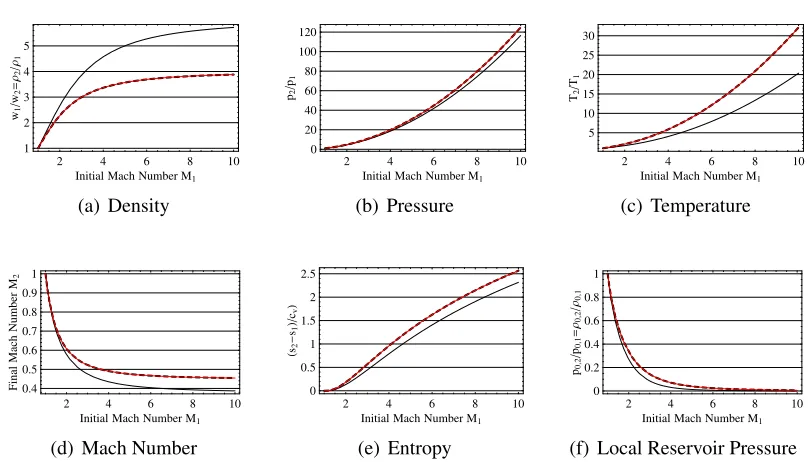
M >= 1 since for smaller Mach numbers isentropic expansion occurs. Figure 1.2 shows plots of the relations (1.36)-(1.40) for Nitrogen (solid black line), Argon (dashed black line), and Helium (solid red line). Since Argon and Helium are both monoatomic gases and, hence, have the same specific heat ratio of 5/3 and because only ratios are plotted the lines for these two gases coincide in all the plots. Again, it can be seen that the density ratio converges towards an asymptotic value while the pressure and temperature ratios grow without limits. Figure 1.2(d) shows the important fact that the flow is always subsonic after the shock with post-shock mach numbers decreasing as initial mach numbers increase. The entropy change normalized to the heat capacity (s2− s1)/cv, Figure 1.2(e), can be used as

a measure for the strength of the shock. To this end, however, it is also possible to define "local" reservoir conditions of a flow w0 = 0, ρ0, p0, ... as those conditions reached by

bringing the flow isentropically to rest, thereby constituting the ideal conditions that could optimally be reached. Here, optimally means that in the case of isentropic compression, no pressure drop occurs and the initial reservoir conditions are obtained again. So, by definition, in an isentropic flow, the local reservoir conditions are constant throughout the flow. For the non-isentropic shock it follows from energy conservation that the local reservoir temperature is also constant but the local reservoir pressure and density drop with the amount of the drop being proportional to the strength of the shock.

ρ0,2 ρ0,1

= p0,2 p0,1

=

"

1+ 2κ

κ+1(M

2₋₁₎

#−κ−11 "

1− 2 κ+1 1−

1

M2

!#−κ−11

(40)

2 4 6 8 10

Initial Mach Number M1 1 2 3 4 5 w1 w2 = Ρ2 Ρ1 (a) Density

2 4 6 8 10

Initial Mach Number M1 0 20 40 60 80 100 120 p2 p1 (b) Pressure

2 4 6 8 10

Initial Mach Number M1 5 10 15 20 25 30 T2 T1 (c) Temperature

2 4 6 8 10

Initial Mach Number M1 0.4 0.5 0.6 0.7 0.8 0.9 1 Final Mach Number M2

(d) Mach Number

2 4 6 8 10

Initial Mach Number M1 0 0.5 1 1.5 2 2.5 H s2 -s1 L cv L (e) Entropy

2 4 6 8 10

Initial Mach Number M1 0 0.2 0.4 0.6 0.8 1

p0,2

p0,1

= Ρ0 ,2 Ρ0 ,1

(f) Local Reservoir Pressure

Figure 1.2: Change of important state variables in a normal shock in a perfect gas (N2, solid black,

Ar, dashed black, He, solid red line) with constant heat capacity.

This equation is plotted in Figure 1.2(f) showing that for low Mach numbers a shock is a quite efficient and for higher Mach numbers a quite inefficient way of decelerating and compressing a flow. Similar to the equations (1.36-1.41), expressions for oblique shock fronts can be derived. The tangential velocity components are preserved by the shock for the shock-normal velocity components as well as for density, pressure, temperature, and local reservoir conditions, equations (1.36-1.41) are still applicable by simply substituting

M sinγ for M where M = M1 is the Mach number before the shock and γ is the angle

between the initial flow velocity and the shock front. Similarly to perpendicular shock fronts, the second principal law prohibits oblique expansion shocks as well. There are two extreme points for the pressure rise in the oblique shock, namely a maximum for

γ = 90◦ corresponding to a normal shock perpendicular to the flow and a minimum for

sinγ = 1/M = sinα with α being the Mach angle. The latter represents the weakest possible distortion of a supersonic flow, so values of M sinγ <1 are not meaningful.

1.1.4 Continuous Flows in Nozzles

(41)

discussed below under which conditions this will happen. However, for the case of interest here, namely a nozzle that is attached to a vacuum chamber, it is clear that no shocks can occur because expansion shocks are impossible. Therefore, in the following only the continuous case is treated extensively.

In order to describe flows that are bound and guided by walls within a 1 D theory it is necessary to introduce the cross section f of the gas-duct into the governing equations. This is most easily done regarding the differential equations corresponding to equations (1.21),(1.22) and (1.23) [139]:

1 w dw dx + 1 ρ dρ dx + 1 f d f

dx = 0 (1.42)

wdw

dx +

1

ρ d p

dx = Y (1.43)

wdw

dx +

di

dx =

dq

dx (1.44)

Here (1.42) is the continuity equation, now including the flow cross section f (m2), (1.43) is the equation of motion including an external volume-force Y and (1.44) states energy conservation. In the case that there are no external forces and no energy or heat flows through the system boundaries, Y = 0, dq/dx = 0, this corresponds to a continuous, isentropic flow ds/dx = 0. Then, by using (1.30) and M = w/c equation (1.43) can be written as

1

ρ dρ

dx = −M

21 w

dw

dx (1.45)

This shows that for small Mach numbers the relative variation of the density is smaller than the relative variation of the velocity and for large Mach numbers vice versa. This leads to the limits of uncompressible flow for very low Mach numbers, and, for high Mach nubmers, to hypersonic flows where the maximum velocity (1.24) has (almost) been reached and stays more or less constant and only density, pressure, and temperature vary strongly.

By combining now equations (1.45) and (1.42) the following relationship between the Mach number and the flow cross section can be derived:

(1−M2)1

w

dw

dx =

1

ρw d(ρw)

dx =−

1

f d f

dx (1.46)

(42)

that for supersonic flows it grows with growing cross section. This effect is exploited in converging - diverging de Laval nozzles as depicted in figure 3. First in the converging sec-tion the flow accelerates up toM= 1 which is reached in the throat. Then, in the diverging nozzle section, the flow is allowed to expand further thereby acquiring supersonic speeds corresponding to M > 1. For M = 1 the flow cross section evidently has a minimum and the flow density a maximum and, therefore, this point in the flow is of special importance because it separates the sub- from the supersonic regime. The flow parameters that the gas obtains at that point are called "critical" parameters and are signed with an asterisk. These critical values can be calculated for the perfect gas with constant heat capacity as follows: Starting from equation (1.23), using (1.13) and assuming that the gas is initially at rest

w0 = 0 one gets

w2

2 +cpT =cpT0 (1.47)

Here, variables with subscript 0 denote initial (reservoir) values. With (1.25) and (1.31) this transforms to

w2₊ 2 κ−1c

2 ₌_w2

max (1.48)

Here, the known critical values for M and w, namely M∗ = 1,w∗ = c∗can be introduced leading to

w2

max=

κ+1

κ−1(w

∗

)2 = κ+1

κ−1(c

∗

)2 = 2

κ−1c

2

0 = (κ+1)cpT∗=2cpT0 (1.49)

and, by exploiting the usual isentropic equations (1.18), (1.19), (1.20), finally the following equations are obtained that now relate the relevant critical flow parameters to the reservoir values:

w∗ ₌

r

κ−1

κ+12cpT0= c0

r

2

κ+1 (1.50)

p∗ p0

= _κ 2 +1

!κ−κ1

(1.51)

ρ∗

ρ0

= _κ₊2 1

!_κ−11

(1.52)

T∗ T0

= _κ₊2

1 (1.53)

ρ∗w∗

ρ0c0

= _κ 2 +1

!₂₍κκ+−11)

(1.54)

(43)

Now that the critical parameters are available, equations (1.13), (1.18) and (1.22) can be used to calculate the flow density in the whole flow domain. Then, one arrives at the following result:

f∗

f =

ρw ρ∗w∗ = M

"

1+ κ−1

κ+1(M

2₋₁₎

#−2(κκ+−11)

(1.56)

A plot of this function is given in Figure 1.3. Due to the continuity relationwρf =w∗ρ∗f∗

the vertical axis in figure 1.3 can also be read as the cross section ratio f∗/_f _thereby

showing that for each cross section two solutions are obtained, one corresponding to the

0 1 2 3 4 5 6

Mach Number 0 0.2 0.4 0.6 0.8 1 Ρ w Ρ *w *

Figure 1.3: Flow density normalized to critical values in a converging -

diverg-ing flow for N2(black solid), Ar (black

dashed) and He (red solid).

subsonic and the other to the supersonic case. From M=0 to M=1 the flow accelerates towards the crit-ical cross section and its flow density grows to its maximum value. As has been shown above, this requires a decreasing flow cross section that finally reaches a minimum value - the nozzle throat - where critical values are obtained. From there on, in order to further increase the Mach number, the flow cross section has to increase again in order to allow for the additional expansion and the corresponding re-duction of the flow density that is necessary to reach the supersonic regime. This converging - diverging nozzle is called a de Laval nozzle and is a very fre-quently used device for producing supersonic gas flows. The mass flow through the nozzle is now given by ˙m∗=ρ∗w∗f∗which evaluates to

˙

m∗= f∗

s

κ 2

κ+1

!κκ+−11

p0ρ0 (1.57)

while the mass flow in general is expressed by

˙

m= f

r

2κ

κ−1p0ρ0

p p0

!1κ

s

1− p p0

!κ−κ1

(1.58)

Since ˙m∗ = _m_˙ _{holds everywhere in the flow domain, relation (1.58) implicitly defines the}

(44)

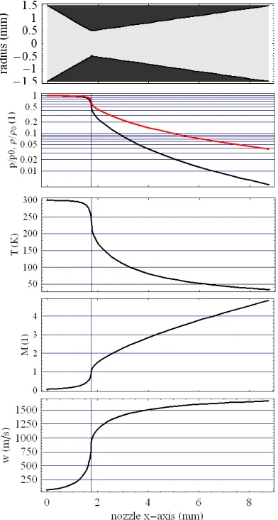
Figure 1.4: Variation of Flow parameters in-side a de Laval nozzle with a cross section

ratio fexit/f∗ = 9. Reservoir parameters: p0

= 5 ×106 Pa = 50 bar, T₀ = 300 K, w0 =

0, medium: Helium. The parameters plotted are: nozzle radius (nozzle contour), pressure (black), and density (red) normalized to their respective reservoir values, temperature (K),

Mach number (1) and flow velocity (m/s)

Figure 1.4 shows plots of the most impor-tant flow parameters along a de Laval noz-zle that is connected to a reservoir containing air at a pressure of 50 bar, a temperature of 300 K (corresponding to an initial density of 1.2×1021 _cm−3_{), and no initial velocity. The}

nozzle contour is also shown. It consists of a converging part with straight conical walls that is 1.75 mm long and has an entrance diameter of 3 mm. The throat diameter is 1 mm and subsequently the nozzle expands again with a straight conical contour to an exit diameter of 3 mm.

Tables 1.1 and 1.2 display numeric values of important flow parameters in the reservoir, at the throat where critical values are obtained and at the nozzle exit of a de Laval nozzle with a cross section ratio fexit/f∗of 9. The pressure

(45)

parameters, the molecular weight M and the heat capacity (for constant pressure)cp. For

air, the average molecular weight is 28.9696g/molandcp is 1006.43 J/kgK, helium has

a molecular weight of 4.0026g/moland acpof 5193 J/kgK. Inspection of the equations

show, however, that in almost all the cases the parameterκ- which is a function of bothcp

and M - is the only medium-dependent parameter. As mentioned above, the significance ofκlies in the fact that 2/(κ−1) corresponds to the number of degrees of freedom of the gas molecules. Its value is 1.4 for Air and 1.67 for helium which corresponds to 5 degrees of freedom for theaverageair molecule and 3 degrees of freedom only the translations -for the point-like helium atom. The main differences between the air flow and the helium flow are the following: The smaller molecular weight of He manifests itself in a much higher exit velocity of 1662 m/s which compares to a theoretical maximum velocity of 1765 m/s. The smaller heat capacity leads to a much smaller exit temperature of 34.1 K as compared to 77.2 K for air which also leads to a higher Mach number for helium of 4.84. The density at the exit is almost the same, the pressures differ by a factor of 2. The mass flow is smaller by a factor of 2.5 for Helium but the volume flow is higher by a factor of 2.8 - another effect of the small molecular weight of helium. If the jet is assumed to

Table 1.1: Flow variables in a de Laval nozzle. Medium: Air. Entrance Diameter 3 mm, Throat

diameter 1 mm. Exit diameter 3 mm. Reservoir parameters: p0=5×106Pa=50 bar,T0=300 K,

w0=0 m/s

Parameter Reservoir Throat Nozzle Exit

Pressure (bar) 50 26.4 0.429

Density (1019cm−3) 121 76.5 4.02

Temperature (K) 300 250 77.2

Mach Number (1) 0 1 3.80

Velocity (m/s) 0 317 670

emanate into vacuum it is not possible within this simple model to predict its evolution outside the nozzle because the flow cross section is not a priori known and cannot easily be calculated. Also, within the nozzle the presented model is accurate only as long as the part of the flow that is affected by the presence of walls is negligibly small in comparison to the flow dimensions. Since the processes within the wall-affected zone, the so-called boundary layer, depend non-trivially on flow parameters like pressure, pressure gradient, velocity, fluid viscosity, and turbulence, there are no sufficiently accurate analytical mod-els that would allow to study this phenomenon in analytical fashion. Therefore, one has to rely on numeric simulation of the flow which will be the central point of the following chapter.

(46)

Table 1.2: Flow variables in a de Laval nozzle. Medium: Helium. Entrance Diameter 3 mm,

Throat diameter 1 mm. Exit diameter 3 mm. Reservoir parameters: p0=5×106Pa=50 bar,T0=

300 K,w0=0 m/s

Parameter Reservoir Throat Nozzle Exit

Pressure (bar) 50 24.4 0.218

Density (1019cm−3) 121 78.4 4.627

Temperature (K) 300 225 34.1

Mach Number (1) 0 1 4.84

Velocity (m/s) 0 882.6 1662

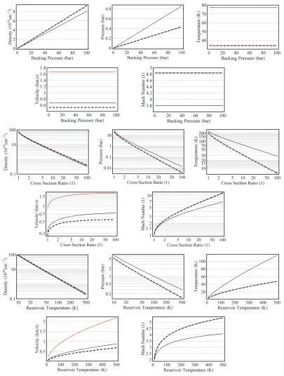
state variables at the exit of the de Laval nozzle on backing pressure, cross section ratio between nozzle throat and exit, reservoir temperature, and on the gas type. In all the plots, the plot for Helium is the solid red, the one for Argon the dashed black, and the one for N2

the solid black line. Since Argon and Helium are both monoatomic gases with the same isentropic exponent it is expected that they show similar behavior. For the upper five and the lower five plots, a cross section ratio of nine was used, for the middle five plots the backing pressure was set to 50 bar. Looking first at the upper five plots in the figure it can be seen that the (particle) density and pressure vary linearly with backing pressure. Since density is measured in particles per cm3 _{and not in} _kg/_m3_{, the two lines for Argon and}

Helium overlap showing exactly the same result. The (static) pressure at the nozzle exit also depends linearly on the backing pressure and, again, Argon and Helium give the same results. Temperature, velocity, and Mach number do not depend on the backing pressure at all. It is apparent that the exit velocity is the only parameter that actually depends on the molecular weight of the gas showing different results for Argon and Helium.

Turning now to the middle five plots, it is clear that by changing the cross section ratio between the nozzle exit and throat, the flow parameters at the nozzle exit readily vary over orders of magnitude, therefore, all plots are in double logarithmic scale. Again, the exit velocity is the only parameter where Argon and Helium show different results. The almost linear behavior of density, pressure, and temperature at the nozzle exit imply a power law dependence on the cross section ratio. The exit velocity rapidly converges to the maximum attainable speed which is given by energy conservation (see 1.25). The fact that the Mach number keeps growing is explained by the falling temperature that lowers the speed of sound.

(47)

Figure 1.5: Variation of relevant state variables with backing pressure (upper five plots), ratio between exit and throat cross sections (middle five plots), and reservoir temperature (lower five

(48)

the Mach number vary with the reservoir temperature, it represents a convenient way of tuning the velocity and Mach number at the nozzle exit. Especially the latter one can be of importance because in the case that supersonic shock fronts are used in the experiment, the ratio of all the flow parameters before and after the shock only depend on the Mach number (see equations 1.36 - 1.40).

1.1.5 Cluster Formation in Supersonic Gas Jets

It is a long known fact that high pressure gas jets emanating into vacuum can be a formidable way of producing large clusters of atoms or molecules, [102], [140] – [143]. This is due to the high densities and low temperatures that are simultaneously reached in such jets. Since de Laval nozzles are especially well suited for reaching both - high density and low pressure - at the nozzle exit, they are especially effective tools for cluster formation. Since the presence of clusters in a gas jet may have an influence on any experiments conducted with these jets, a short analysis of the cluster production in supersonic gas jets is presented. Since dimers are the first step in cluster formation, the dimer mole fraction XA2

rep-resents a meaningful measure for the number of clusters to be expected in a gas jet. The dimer formation goes on continuously from the nozzle throat diameter downstream until the so-called sudden freeze surface is reached beyond which no more significant conden-sation into clusters occurs any more [140]. The position of this surface is essentially a function of temperature and can be assumed to lie several nozzle diameters away from the nozzle exit in the case of small diameter ratios (< 4:1) of the de Laval nozzle. Therefore, the final dimer mole fraction can be regarded an upper limit of the dimer content close to the nozzle exit. In order to calculate the final dimer mole fraction the following empirical formula is given in [140]:

XA2=

1 2        

ρPσ3

ε kBT

!7₅

d∗ σ

!2₅        5 3 (1.59)

Here, ρPis the gas number density, σis the atom size,εis the potential well depth, kB is

Boltzman’s constant, d∗is the critical (smallest) diameter of the nozzle. Values for these parameters can be found in [140] and [144]. For Helium the following values are used:

σ = 2.66×10−10 _m,ε/_k

B = 10.9 K, and for Argon σ= 3.33×10−10 m,ε/kB =144.4 K.

In the case of a de Laval nozzle for d∗the following expression is substituted [140], [141]:

deq∗ = 0.736dCcot(α), γ= 5/3 (1.60)

deq∗ = 0.866dCcot(α), γ= 7/3 (1.61)

(49)

1 2 5 10 20 50 100

p0HbarL

0.1 1 10 100 1000

dC

H

mm

L

(a) Dimer mole fraction of 0.01 for Argon

1 2 5 10 20 50 100

p0HbarL

1.´106

1.´107

1.´108

1.´109

1.´1010

dC

H

mm

L

(b) Dimer mole fraction of 0.01 for Helium

Figure 1.6: Plots of critical nozzle diameters and backing pressures that lead to a dimer mole fraction of 0.01 which is considered as the onset of clustering. (a) Argon, (b) Helium.

[140], [145], considerable clustering sets in for mole fractions larger than 0.01. This is shown in figure 1.6 where those value pairs of dCand p0are plotted that correspond to a

value of XA2of 0.01. In order to have no clusters, parameters below the lines have to be

(50)