Spectrally Resolved Longitudinal Spatial Coherence Interferometry.

ABSTRACT

WOODARD, ETHAN ROBERT. Spectrally Resolved Longitudinal Spatial Coherence Interferometry. (Under the direction of Michael Kudenov).

In this dissertation, an alternative imaging technique is presented which uses longitudinal

spatial coherence interferometry to encode a scene’s spatial information onto the source’s

power spectrum. By spectrally resolving the output using a spectrometer, a channeled

spectrum is measured. Fourier transformation of the channeled spectrum yields a

measurement of the incident scene’s angular spectrum. Theory is presented to exhibit

analogies to conventional Fourier transform spectroscopy of the power spectrum.

Experimental validation of the technique is demonstrated, using a Fabry-Pérot etalon, for

the reconstruction of one-dimensional sinusoidal and randomly generated angular spectra.

This technique is further developed to create an alternative technique for channeled

polarimetry which uses longitudinal spatial coherence interferometry to encode a scene’s

angularly dependent polarization information onto the source’s power spectrum. As before,

a Fourier transformation of the measured channeled spectrum, in combination with

reference beam calibration techniques, yields a reconstruction of the incident scene’s

angular Stokes parameters. Experimental validation of the technique is demonstrated, using

a Fabry-Pérot etalon, for the recovery of one-dimensional linearly polarized scenes and a

step-function scene between two linearly polarized states.

An alternative approach to encode a scene’s angular information onto the power

spectrum is presented, which leverages the dispersive properties of glass materials. By

implementing two glass materials with different dispersion characteristics within a

incident angles adds constructively at a single wavelength. This phenomenon generates a

region of coherence in a spectrally resolved measurement, whose envelope contains the

angular information of the scene. Theory is presented for the spatial-spectral multiplexing

technique, as well as modeling and experimental results from the investigation of various

interferometer schemes. Details of the resolution and operational limitations associated

with the technique are offered.

Finally, a discussion of the future implications of the aforementioned techniques is

presented. The researcher offers insight into several applications in which spectrally

resolved longitudinal spatial coherence interferometry may have future impact. These

techniques include lensless imaging, three- and four-dimensional scene reconstruction, and

propagation of a scene’s spatial and polarization information through multimode optical

© Copyright 2017 Ethan Robert Woodard

Spectrally Resolved Longitudinal Spatial Coherence Interferometry

by

Ethan Robert Woodard

A dissertation submitted to the Graduate Faculty of North Carolina State University

in partial fulfillment of the requirements for the degree of

Doctor of Philosophy

Electrical Engineering

Raleigh, North Carolina

2017

APPROVED BY:

_______________________________ ______________________________

Michael Kudenov Robert Kolbas

Committee Chair

_______________________________ ______________________________

ii

DEDICATION

iii

BIOGRAPHY

Ethan Woodard was born in Columbia, South Carolina to Cliff and Lisa Woodard. After

high school, Ethan attended Presbyterian College for his undergraduate studies and

graduated in 2013 with a B.S. in physics and a B.S. in applied mathematics. He then moved

to Raleigh, North Carolina to attend North Carolina State University in pursuit of an M.S.

in electrical engineering, later transferring to the Ph.D. program under the advisement of

Michael Kudenov. His research interests in the Optical Sensing Lab were related to

iv

ACKNOWLEDGMENTS

First and foremost, I would like to thank Dr. Kudenov for all of his mentoring during my

time at NC State. I also extend thanks to my fellow OSL members who were always willing

to talk things out at the white board. Lastly, I would like to thank my family and friends

v

TABLE OF CONTENTS

LIST OF TABLES………....viii

LIST OF FIGURES……….ix

1.0 Chapter 1: Introduction ... 1

2.0 Chapter 2: Snapshot Spectrally Resolved Longitudinal Spatial Coherence Interferometry ... 7

2.1 Introduction ... 7

2.2 Theory ... 7

2.2.1 Coherence ... 16

2.2.2 Comparison with Conventional Longitudinal Spatial Coherence Interferometry ... 22

2.3 Experimental Setup ... 24

2.3.1 FPE Simulation ... 26

2.3.2 Alignment of Fabry-Pérot Etalon and SLM Carrier Frequency ... 27

2.3.3 Alignment Procedure ... 29

2.4 Experimental Results... 32

2.4.1 Sinusoidal Angular Spectra... 32

2.4.2 Random Angular Spectra ... 36

2.4.3 Error Analysis ... 38

2.4.4 Angular Resolution Analysis ... 40

2.5 Radiometric Analysis ... 42

2.6 Conclusion ... 48

vi

3.1 Introduction ... 49

3.2 Theory ... 51

3.3 Recovery of Angularly Dependent Stokes Parameters ... 58

3.3.1 Reference Beam Calibration ... 58

3.3.2 False Signature Artifact Reduction Technique ... 58

3.4 Experimental Setup ... 60

3.4.1 Alignment Procedure and Methods ... 62

3.5 Experimental Results... 64

3.5.1 First order analysis ... 64

3.5.2 Uniform Stokes Scenes ... 66

3.5.3 Stokes Step Function... 72

3.6 Conclusion ... 74

4.0 Chapter 4: Spatial-spectral Multiplexing using Nonlinear Dispersion ... 76

4.1 Introduction ... 76

4.2 Theory ... 76

4.3 SSM Architectures, Experimental Setups and Results ... 83

4.3.1 Michelson Interferometer ... 84

4.3.2 Mach-Zehnder Interferometer ... 92

4.3.3 Polarization Grating-based Interferometer ... 100

4.3.4 Miscellaneous System Architectures ... 114

4.4 Reconstruction Algorithm for Nonlinear Channeled Spectra ... 120

4.4.1 Simulations of Linear and Nonlinear Optical Path Differences ... 121

vii

4.5 Angular Resolution Analysis ... 143

4.6 Comparison of Angular Resolution of Lens to Fabry-Pérot System ... 153

4.7 Tolerancing and Aberrations ... 155

4.7.1 Tolerancing of Beamsplitter Terminus ... 155

4.7.2 Wavefront Aberrations in Interferometers ... 161

5.0 Chapter 5: Future Work ... 168

5.1 Lensless Imaging ... 168

5.2 Propagation of a Scene’s Spatial and Polarimetric Information through Optical Fibers ………...169

5.3 Reconstruction of three- and four-dimensional object space data ... 171

6.0 Conclusion ... 173

viii

LIST OF TABLES

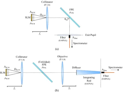
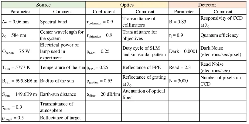
Table 1. Parameters for Radiometric Calculations for the FPE system ... 45

Table 2. RMS Error calculations for reconstruction of normalized Stokes parameters for

uniform, linearly polarized scenes ... 71

Table 3. RMS Error calculations for reconstruction of normalized Stokes parameters for

the step function scene ... 74

Table 4. Glass analysis data for several pairs of potential glass materials for the

PG-interferometer. ... 110

Table 5. Spectral resolutions required to resolve maximum frequencies in channeled

ix

LIST OF FIGURES

Fig. 1. (a) Michelson interferometer configured to measure the spectrum of a source. (b)

Interference pattern, measured on the FPA as a function of OPD; (c) Fourier transform of

the data in (b), yielding the source’s power spectrum. ... 8

Fig. 2. (a) Michelson interferometer configured to measure the angular spectrum of a

uniform source. (b) Spectrally resolved interference pattern, measured on the spectrometer,

as a function of a measurement variable ν that depends on wavenumber σ; (c) Fourier

transform of the data in (b), yielding the source’s angular spectrum. ... 12 Fig. 3. Channeled spectrum simulated for MI with linear ν (red line) relationship,

illustrating low coherence in the detectable region of the spectrum (green shading). ... 16

Fig. 4. FTAS which relays an arbitrary object’s angular spectrum onto an SLM with

transmittance τS. Light is then collimated into the tilted MI, where the spectrally resolved

interference is detected using a spectrometer. ... 18

Fig. 5. Channeled spectrum for wavenumbers spanning 0 mm-1 (λ = ∞ nm) to 2857 mm-1 (λ = 350 nm). The highlighted region signifies wavenumbers spanning 1000 to 2500 mm-1

(λ spanning 1000 to 400 nm). Measurement of (a) the cosine carrier frequency ν0 and (b)

an additional modulation on ν0with a frequency Δν. ... 20

Fig. 6. (a) Visibility peaks simulated for a FZP designed for λ0 = 633 nm and high

coherence at Δz = 2 mm. (b) Simulated spectrally resolved channeled spectrum for

2Δz = 4 mm. ... 23

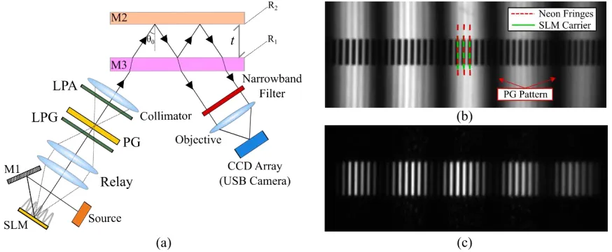
Fig. 7. (a) Schematic of the experimental configuration for the FPE-based interferometer;

x Fig. 8. (a) Schematic of the spectrometer that was used for our experiments; (b) photo of

the spectrometer on the benchtop. ... 26

Fig. 9. (a) Calculation of FPE reflectance vs. wavelength (solid blue line), for t = 14 μm

and an angle of incidence of 52°, and the coating reflectance (dashed orange line), as

obtained from Thorlabs at an incidence angle of 45° [0]. (b) Fourier transform of the FPE

reflectance spectrum of (a), but for a t = 100 μm cavity. ... 27

Fig. 10. (a) Schematic for FPE alignment configuration, in which the xenon arc lamp source

was replaced with a low pressure neon gas discharge lamp. A camera is also used to directly

observe the light from the SLM and source. (b) Image of the SLM’s carrier fringe

superimposed onto the fringe, observed by residual spectrally narrow band light reflected

off the SLM’s surface. A spatial beat frequency is observed when the FPE’s thickness is

not ideal. (c) Image of an aligned system. In this case, maximum coherence would occur

at a wavelength equal to the neon gas lamp’s filtered emission wavelength at 633 nm. .. 29

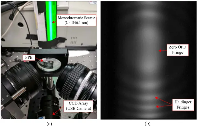
Fig. 11. (a) Setup for aligning the FPE for maximum contrast. A USB camera focused at

infinity is used to image the Haidinger fringes generated by a monochromatic source. (b)

Image of the Haidinger fringes generated by the etalon. ... 30

Fig. 12. Image of the illumination setup for collimation and alignment of the SLM carrier

frequency to the Haidinger fringes within the etalon... 31

Fig. 13. (a) Image of the setup for ensuring collimation of the carrier frequency and (b) an

acquired image from the SLM carrier frequency pattern superimposed on Haidinger fringes

xi Fig. 14. Sinusoidal angular spectra that were loaded onto the SLM (solid blue line) and the

associated envelope function (black dashed line) that corresponds to the spatial information

being measured. ... 33

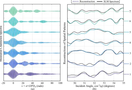
Fig. 15. Measured results. (a) Channeled spectra. The spectra are illustrated from highest

to lowest spatial frequency from top to bottom. (b) The reconstructed results (dotted

colored lines), after Fourier transformation and Mertz phase correction, plotted with the

sinusoidal angular spectra (solid black lines). ... 35

Fig. 16. Random angular spectra that were loaded onto the SLM (solid blue line) and the

associated envelope function (black dashed line) that corresponds to the spatial information

being measured. ... 36

Fig. 17. Measured results for random spectra. (a) Channeled spectra. The spectra were

randomly selected from an experiment containing 100 different random spectra. (b) The

reconstructed results (dotted colored lines), after Fourier transformation and Mertz phase

correction, plotted with the randomly generated angular spectra (solid black lines). ... 38

Fig. 18. (a) RMS error versus spatial frequency factor N for the sinusoidal angular spectra

and (b) (a) RMS error versus spectrum index for the band-limited random angular spectra.

... 39

Fig. 19. Schematic used for radiometric and SNR calculations for (b) the optimal system

setup, sampling within the exit pupil of the objective, and (b) the ‘unfolded’ experimental

xii Fig. 20. SNR versus integration time calculated based on the optical power collected at the

aperture of the fiber for the optimal and experimental FTAS systems under (a) laboratory

conditions and (b) a simulated overfilled target under passive solar illumination. ... 46

Fig. 21. SNR versus integration time calculated for the optimal and experimental setups of

the FTAS systems using the grating spectrometer under (a) laboratory conditions and (b) a

simulated overfilled target under passive solar illumination. ... 47

Fig. 22. Model of the CP technique used by Oka and Kato [33], in which high order

retarders are used to generate cosinusoidal carrier frequencies which encode the incident state of polarization onto the source power spectrum as a function of wavenumber, σ. .. 50

Fig. 23. Simple model of the proposed CP technique, in which angularly dependent Stokes

parameters are amplitude modulated onto the source power spectrum using an SLM and

sinusoidal PG. Spectrally resolving the output from a linear CS modulator generates a CS

which contains polarization information of the scene. ... 51

Fig. 24. Schematic of a linear channel spectrum modulator (e.g. titled MI) used to encode

polarization information onto the source’s power spectrum. The SLM provides the

sinusoidal carrier frequency while a polarization grating (PG) of period Λ creates the

sinusoidal envelope used to generate channels within the measured spectrum. ... 52

Fig. 25. Schematic of the intermediate image plane of the optical system in Fig. 24. ... 52

Fig. 26. Simulated channeled spectrum for system in Fig. 24 with PG period Λ = 2240 μm.

Magnified view of the three channels separated in ν space by the phase term, ϕ1, present

xiii Fig. 27. In CP, (a) the S0 component of the source is present near the centerburst, while (b)

the other Stokes parameters are encoded into displaced channels. Since spectral

measurements are a superposition of these components, (c) aliasing will occur when

centerburst modulations are present in the side channels. ... 59

Fig. 28. (a) Schematic and (b) optical table setup of the FPE-based proof of concept system

used for the channeled spectropolarimetry technique. ... 62

Fig. 29. (a) Schematic for FPE alignment configuration, in which the xenon arc lamp source

was replaced with a low pressure neon gas discharge lamp. A camera is also used to directly

observe the light from the SLM and source. (b) Image of the SLM’s carrier fringe

superimposed onto the fringe, observed by residual spectrally narrow band light reflected

off the SLM’s surface. In this aligned system case, maximum coherence would occur at a

wavelength equal to the neon gas lamp’s filtered emission wavelength at 633 nm. (c) Actual

image of the modulated carrier frequency pattern (illuminated by white light) which would

generate channels in the experimental setup. ... 64

Fig. 30. (a) Scaled (×1.7) experimentally acquired CS superimposed on simulated CS for

LPG(0º), LPA(90º). (b) Magnified view of channel C1 in two experimentally acquired CS

for LPG(0º) and LPG(90º). ... 65

Fig. 31. (a) Image of the sinusoidal pattern of period Λ for the PG used in proof of concept

experiments. (b) Image of the analyzers, LPA(0º) and LPA(90º), used to implement the

ART calibration (red arrows denote orientation axis). ... 67

Fig. 32. Processed channeled spectra for a reference, LPG(0º), and sample, LPG(45º), data

xiv measurements for LPA(0º). The yellow spectra are the higher resolution spectrum used in

the ART. ... 68

Fig. 33. Unmodulated spectra used to calculate the weighting factor Γ(ν). ... 69

Fig. 34. Simulation (Sim, solid lines) and experimental (Exp, dashed lines) reconstruction

results for the normalized angularly dependent Stokes parameters, S1/S0 and S2/S0, versus

angle of incidence for linearly polarized scenes: (a) 67.5º, (b) 90º, (c) 135º, and (d) 157.5º.

... 70

Fig. 35. Image of the Stokes step function created by two linear polarizing generators

oriented such that the scene is define as a step between an S1 to S2 polarization state. Model

of the Stokes step function used in numerical simulation of channeled spectra and simulated

reconstructions. ... 72

Fig. 36. Simulation (‘Sim’, solid lines) and experimental (‘Exp’, dashed lines)

reconstruction results for the normalized angularly dependent Stokes parameters, S1/S0

(blue lines) and S2/S0 (red lines), versus angle of incidence for the Stokes step function

scene. State of polarization across the FOV goes from (a) 0º to 135º, (b) 0º to 45º, (c) 45º

to 0º, and from (d) 135º to 0º. ... 73

Fig. 37. Channeled SSM technique using a tilted Michelson interferometer. (a) A tilted MI

accepting multiple angles from the scene. (b) The channeled spectrum created by the MI

and (c) its respective angular spectrum via Fourier transform. ... 77

Fig. 38. Channeled spectrum generated by tilted white-light Michelson interferometer (blue

curve). Region of reduced contrast at visible wavenumbers where the spectrometer

xv Fig. 39. Angular coherence compensation for channeled SSM. (a) A tilted MI compensated

for a single wavelength defined by the intersection of the dispersion curves of the two glass

plates in (b). (c) Simulated channeled spectrum generated by the MI system in (a). ... 80

Fig. 40. Designs for the dual-glass type interferometer systems include the conventional

(a) and modified (b) Michelson interferometer, the conventional (c) and modified (d)

Mach-Zehnder interferometer, and the diffraction-based polarization grating (e)

interferometer. ... 84

Fig. 41. A Michelson interferometer with a plate of glass (or dispersion fluid) in each arm.

One plate has a higher relative dispersion (lower Abbe number) than its counterpart. .... 85

Fig. 42 (a) Dispersion curves for glass windows N-LAK33A and N-SF14. (b) Simulations

of channeled spectra for the ideal case (t1 = t2) and the actual case (t1≠ t2). ... 87

Fig. 43. (a) Schematic of MI system for SSM proof of concept experiment. (b) Optical

table setup for SSM experiment, sampling the (exit) pupil plane of the collimator. ... 88

Fig. 44. Flat field corrected channeled spectra for 3 positions across the defocused image

of the scene slit (i.e. exit pupil). ... 90

Fig. 45. Simulated (blue curve) versus experimental (red curve) channeled spectra for the

proof of concept MI system. ... 91

Fig. 46. Magnified view of the processed experimental data near the centerburst (a) and at

longer wavelengths (b). ... 92

Fig. 47. Two plane-parallel plate model of MMZ interferometer system. ... 94

Fig. 48. (a) Schematic and (b) optical table setup for a proof of concept experiment using

xvi Fig. 49. Illustrations of the three techniques used for aligning the MZ interferometer for

proof of concept experiments... 96

Fig. 50. Channeled spectrum acquired by the OSA spectrometer from interference

generated in the dispersive MZ interferometer. ... 98

Fig. 51. Channeled spectrum acquired by the FTIR spectrometer from interference

generated in the dispersive MZ interferometer. ... 100

Fig. 52. Design of a PG-based channeled SSM system containing four dispersive materials

and four polarization gratings. ... 101

Fig. 53. Design of PG-based system with two dispersive materials between respective sets

of PGs with period Λ. The rays are shown for an unbalanced system at a wavelength for

which the refractive indices of glasses G1 and G2 are unequal. ... 103

Fig. 54. PG-based system, depicted for a 20 degree angle of incidence at 633 nm. The PG

grating periods are all equal to Λ = 4 microns. All dimensions in mm or degrees. A zoomed

in region of the two exiting rays is displayed in panel (P1)... 106

Fig. 55. Experimental setup for establishing proof of concept results for the SSM technique

and resolution data using a PG-based interferometer. ... 107

Fig. 56. Analysis of spectral content for the LAK8/SF1 glass pair at wavenumbers near the

Fraunhofer spectral lines. Separation of the data cursors is an approximation of the spectral

resolution needed to resolve the frequency content. ... 112

Fig. 57. Simulation of the interference fringes generated at the output of the PG-based

xvii Fig. 58. A compact Mach-Zehnder interferometer with visible white light interference

fringes visible with the preliminary setup for measuring a channeled spectra from the

compact Mach-Zehnder. ... 115

Fig. 59. Dispersion curves for the ordinary and extraordinary rays of CdS. ... 117

Fig. 60. Simulation of the channeled spectrum and phase, ν = σOPD(σ), generated by the

o and e rays of a CdS retarder based on the relationship in the dispersion curves between

no(λ) and ne(λ) ... 118

Fig. 61. (a) Schematic of potential proof of concept SSM system using a birefringent

crystal. (b) Preliminary experiment of birefringent system using a CdS retarder as the

dispersive material. ... 118

Fig. 62. Example of a general situation for a channeled spectrum (blue spectrum) with a

nonlinear OPD dependence (green line) versus a linear OPD dependence (red line). ... 121

Fig. 63. Simulated channeled spectrum (blue) plotted with the linear ν (red) against

wavenumber from σ = 0 m-1 toσ = 2.5 × 106 m-1. Channeled spectrum is simulated with a uniform angular spectrum of 1,000 planes waves in the FOV from -2º to +2º, with an initial

interferometer tilt of 20º. ... 123

Fig. 64. Fourier transform of a double-sided channeled spectrum formed by a linear ν

plotted with respect to 1/δν. Important ranges in frequency bandwidth are represented on

the graph... 125

Fig. 65. Simulated channeled spectrum (blue) plotted with the absolute magnitude of the

xviii Fig. 66. Close up of the quadratic ν channeled spectrum for the spectral range of σ = 0.6 × 106 _m- 1 _to σ _{= 1.1 × 10}6 _m- 1_{. Illustrates the region near local maximum (or}

minimum) of the quadratic v phase factor that exhibit fringes of lower frequency and

stationary phase. ... 129

Fig. 67. Normalized channeled spectrum and nonlinear (quadratic) ν over the truncated

spectral range of σ = 1.0 × 106 m- 1 to σ = 2.5 × 106 m- 1. ... 132

Fig. 68. Plot of the original nonlinear phase ν versus the third-order polynomial fitting of

the truncated data. ... 133

Fig. 69. Plot of the truncated nonlinear ν versus the linear approximation of ν from obtained

via the zero crossing and the maximum and minimum values of the nonlinear ν. ... 135

Fig. 70. Plot of the linearly interpolated channeled spectrum after truncation of

wavenumbers to obtain the content between maximum and minimum values of the

nonlinear ν. Channeled spectrum initially contained 100,000 wavenumber samples before

truncation. ... 139

Fig. 71. Reconstructed angular spectrum from direct FFT implementation of the linearly

interpolated channeled spectrum of 100,000 wavenumber samples before truncation. . 139

Fig. 72. Close up of a single side of the reconstructed angular spectrum. Note the jagged

sampling at the peaks of the bandwidth. ... 141

Fig. 73. Reconstructed angular spectrum of linearly interpolated channeled spectrum

(100,000 wavenumbers, 1,000 plane waves over the FOV of θ = -5º to θ = +5º). ... 142

Fig. 74. Angular spectrum reconstructed from a nonlinear channeled spectrum of 500,000

xix Fig. 75. Rotation Fabry-Pérot cavity illuminated by a point source creating two-beam

interference at the observation plane. The optical paths of the two interfering rays are

represented as R1 (black line) and R2 (blue line). ... 146

Fig. 76. Angular resolution, dθi, for an FPE for three different indices of refraction,

n1 = {1.5, 1.6, and 1.7}. ... 148

Fig. 77. PSF of an ideal lens for a single wavelength, λ = 500 nm. ... 150

Fig. 78. PSF of lens plotted for five values of λ in the visible range with λ = 400 nm setting

the lower bound of the angular resolution. ... 152

Fig. 79. Total intensity of PSF (black dashed line) represented as the summation of all the

component wavelengths of the spectrum, unscaled version to show relative magnitude on

left and zoomed-in version to show possible zero-crossings on right. ... 152

Fig. 80. Angular resolution of ideal lens and general FP versus angle of incidence (θ0 = 5°

to θ0 = 45°) for σmax = 2.50 × 106 m-1 for multiple values of OPDmax (top). Zoomed-in

version of the same plot around the angles of incidence for which f = D for the lens

(bottom)... 155

Fig. 81. Dispersion curves of potential glass options (N-LAK8 and N-SF1) based on

Sellmeier equations and known coefficients. Intersection represents design wavelength of

the MI system. ... 157

Fig. 82. Depiction of beamsplitter terminus, with t representing the thickness of the offset.

xx Fig. 83. Simulations of channeled spectra generated by a Michelson interferometer for

equal path lengths (t1 = t2 = 2 mm) with (red curve) and without (blue curve) a beamsplitter

terminus... 159

Fig. 84. Images of the white light interference patterns generated by a Michelson

interferometer for two different sets of dielectric mirrors. ... 160

Fig. 85. Zemax ray trace of MI used with MZDDE and the MATLAB modeling routine.

... 162

Fig. 86. Diagrams of two different scenarios for modeling the effects of wavefront

aberrations in the MI system. (a) Both arms of the MI experience the same added wavefront

error. (b) Same initial wavefront error, but one arm has more wavefront error added. .. 163

Fig. 87. Schematic of the breakdown evaluation of the wavefront error contributed by each

surface of a single arm of the MI system. ... 164

Fig. 88. Schematic of an optical system for spectrally resolved LSCI which replaces the

SLM and collimating lens with geometric phase gratings. ... 169

Fig. 89. Schematic of future application of technique for one-dimensional imaging through

multimode optical fibers. ... 170

Fig. 90. Schematic of the optical model used to develop the SSM reconstruction algorithms

1

1.0 Chapter 1: Introduction

Encoding information onto different dimensions has been investigated in the fields of fiber

optics and communication [1-5], medical imaging [6,7], microscopy [8-10], and remote

sensing [11,12]. Techniques presented in the past have relied on an analog of Hadamard

multiplexing to encode spatial information onto the incident power spectrum; e.g., by use

of filter arrays or masks onto which an object is imaged. In this work, we focus on the

encoding of a scene’s angular spectrum onto a broadband power spectrum by use of

phase-based multiplexing. This is achieved by leveraging longitudinal spatial coherence and the

angular sensitivity of a Fabry-Perot etalon to modulate incident angular information onto

the coherence of the source power spectrum. In this way, each spatial component of the

angular spectrum has a unique frequency in the measured channeled spectrum [13]. The

proposed technique has parallels to Fourier transform spectroscopy [14] in which

interferometric systems are used to modulate the source’s power spectrum onto an angular

spectrum (or spatial axis). Similar to Fourier transform spectroscopy, reconstructing the

angular spectrum can be achieved using a Fourier transform relationship.

In the field of fiber optics and communication a different approach to

spatial-spectral encoding or multiplexing is used to increase the amount of information that can be

transmitted along the fiber. Since fibers have low spatial resolution and complex transfer

functions versus angle, incident spatial information is encoded onto a different space, such

as wavelength [3] or time [4]. In many cases, the spatial-spectral encoding and decoding

2 Armitage et. al. [2] proposed a technique for wavelength multiplexing using dispersive

prisms to encode a one-dimensional object onto the spectrum of a white-light point source.

The prisms served to disperse the white light spectrum across a one-dimensional slit along

the object such that each spatial point was encoded onto a different wavelength before

propagating through a non-imaging light pipe. Meanwhile, Mendlovic et. al. [5] devised a

wavelength multiplexing technique which relied on diffractive structures to create the

spectral spreading across both one- and two-dimensional objects. In this instance, the

diffraction gratings were designed such that each spatial location or pixel across the object

was mapped to a specific wavelength before transmitting through a single-mode fiber. The

decoding process, used to reconstruct the object, also relied on diffractive elements to

convert the individual wavelengths back into their corresponding spatial components.

More recently the research of Barankov and Mertz [7] has demonstrated the use of

spread-spectrum encoding to create high-throughput two-dimensional images of broadband

white-light illuminated sources through single-mode fibers. By using low-finesse Fabry-Perot

etalons as the spread-spectrum encoder, incident ray angles from an extended spatial

distribution are given a unique spectral code across the full spectrum of the source.

Reconstructing the object requires numerical decoding, rather than optical decoding, as

seen in the prism and diffraction grating systems.

Unlike the wavelength multiplexing created using dispersive prisms or diffractive

optical elements, our proposed system relies on interferometric techniques to encode the

angular information onto the power spectrum. In this way, individual components of the

3 frequencies or phases across the entire spectral range of the source. Our technique is more

similar to the work of Barankov and Mertz; however, the basis of our encoding procedure

relies on Dirac delta functions in the spatial domain being related to sinusoids in the

spectral domain, rather than pseudo-random but unique spectral codes used in their

spread-spectral encoder. This allows for a direct Fourier transformation relationship between the

measured channeled spectrum and the reconstruction of the incident angular spectrum.

Longitudinal spatial coherence is used here to refer to coherence between two

points along the optical axis as derived by interpretation of the Van Cittert-Zernike

Theorem [0]. Many researchers have studied the application of longitudinal spatial

coherence to the fields of optical coherence profilometry and tomography [16-20]. Rosen

and Takeda [17] demonstrated the use of longitudinal spatial coherence for surface

profilometry by shifting the degree of spatial coherence with modulations of the source’s

intensity distribution. The researchers used a Michelson interferometer illuminated with

quasi-monochromatic spatially incoherent light to measure the gap between a reference

and test mirror. However, instead of translating one of the mirrors along the longitudinal

axis to determine peaks in coherence, spatial masks, defined by Fresnel zone plates, were

used to modulate the source distribution. The height of the mirrors was thus determined by

a relationship between peaks in spatial coherence and the grating constant or fringe

frequency of the zone plates. Similarly, Wang et. al. [18] continued the preceding work to

demonstrate an interferometric system for tomographic applications. Using a spatial light

4 evident at surface heights which were spatially coherent with Fresnel zone plate-like

sources.

In our interferometric techniques, the concept of longitudinal spatial coherence is

used to maximize the contrast in fringes observed within the measured channeled spectrum.

The spatial frequencies of a source’s angular spectra are coherently matched to the

transmission peaks of monochromatic Haidinger fringes generated within a Fabry-Perot

etalon. When a spectrometer is used to measure the channeled spectrum, maximum

coherence occurs at a wavelength which observes resonance along the longitudinal axis of

the cavity. A channeled spectrum refers to a sinusoidally modulated white-light spectrum

and forms the basis for the measured output of the proposed technique. An example of the

use of a channeled spectrum to recover information is presented by Oka and Kato [11], in

which the state of polarization of a scene is modulated onto the power spectrum of the

source. Using birefringent retarders to create phase retardations along the longitudinal axis

as a function of wavenumber, three quasi-cosinusoidal components are generated which

carry information about the polarization state of the scene. These components appear as

discrete channels along the axis of path difference for the system, and a readily accessible

to demodulate the polarization information of interest. To create discrete channels within

the spectrally resolved measured signal of our system, a cosinusoidal spatial carrier

frequency is used to shift coherence into the detectable region of the spectrum. The carrier

frequency is then amplitude modulated with a spatial envelope to encode angular

information into the channeled spectrum’s coherence. Recovery of the envelope is readily

5 The research of this dissertation as detailed in the following chapters has evolved

several current state-of-the-art techniques in the research fields related to Fourier transform

spectroscopy, longitudinal spatial coherence, and channeled imaging polarimetry. Related

to Fourier transform spectroscopy, this dissertation work has led to the first formal

demonstration of a Fourier transform angular spectrometer (FTAS), which allows for the

recovery of angular spectrum from a spectral measurement, with strong analogies in terms

of resolution and reconstruction algorithms. Conventional longitudinal spatial coherence

interferometry has primarily focused on resolving depth information from two-dimensional

measurements of spatial coherence functions. The work of this dissertation now allows for

acquisition of amplitude and phase information of an optical system’s pupil from

measurements of one-dimensional spatial coherence functions, which leads to the recovery

of a scene’s spatial and polarimetric information. Lastly, with conventional channeled

imaging polarimetry, recovery of spatially dependent polarization information requires a

Fourier transformation of a two-dimensional image. The technique developed in this

research can now recover angularly dependent polarization information directly from

spectrally channeled measurements, with only the polarimetric information of interest

retrieved directly from the measurement domain.

In chapter 2.0, the researcher introduces the technique of snapshot spectrally

resolved longitudinal spatial coherence interferometry by deriving the theory and drawing

parallels to conventional Fourier transform spectroscopy. The experimental setup and

alignment procedure are detailed, and experimental results for the reconstruction of

6 experimental results, and a discussion of the angular resolution and radiometric tradespace

is offered. Chapter 3.0 details the development of the technique for channeled polarimetry,

which allows for the recovery of angularly dependent polarization information from

spectral measurements. Theory and calibration techniques are outlined, followed by the

experimental setup and alignment procedure for the laboratory-based optical system.

Experimental results for the recovery of one-dimensional linearly polarized scenes and a

step-function scene between two linearly polarized states are presented.

In chapter 4.0, the researcher introduces an alternative technique for encoding a

scene’s angular spectrum onto the power spectrum which leverages the nonlinear

dispersion characteristics of glass materials. Theory for the spatial-spectral multiplexing

technique and results from the investigation of several interferometer architectures are

presented. A reconstruction algorithm for nonlinearly sampled experimental measurements

is outlined, followed by discussion of the resolution and operational limitations associated

with the technique.

Finally, in chapter 5.0, the researcher offers insight into the implications of the

spectrally resolved longitudinal spatial coherence interferometry technique for future

applications. The applications for which the technique has the potential to make an impact

include lenless imaging, imaging through multimode optical fibers, and three- and

7

2.0 Chapter 2: Snapshot Spectrally Resolved Longitudinal Spatial Coherence Interferometry

2.1 Introduction

In this chapter, the researcher introduces an alternative imaging technique which encodes

a scene’s angular information onto the source’s power spectrum. Theory for the

interferometric technique for angular-spectral encoding is derived with parallels to Fourier

transform spectroscopy. Details of the experimental design and procedures for validation

of the technique are presented, followed by experimental validation based on the

reconstruction of sinusoidal and random angular spectra.

2.2 Theory

In a conventional Fourier transform spectrometer, or as we will refer to it as a Fourier

Transform Power Spectrometer (FTPS), incident frequency components of the power

spectrum are represented as unique spatial frequencies after two-beam interference. A view

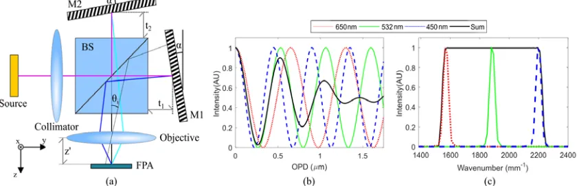
of a typical FTPS is illustrated in Fig. 1 (a), in which a Michelson interferometer (MI), with

tilted mirrors, is used to create a spatially varying optical path difference (OPD) on a focal

plane array (FPA). In this system, light from a source is collimated through a collimator

into a beamsplitter (BS). This redirects the light onto two mirrors, M1 and M2, which are

tilted by an angle α. Light is reflected from these tilted mirrors into an objective lens, which

8

Fig. 1. (a) Michelson interferometer configured to measure the spectrum of a source. (b) Interference pattern, measured on the FPA as a function of OPD; (c) Fourier transform of the data in (b), yielding the source’s power spectrum.

The OPD, as a function of FPA spatial position, can be represented [21] as

( )

OPD y = y α (1)

The detected interference pattern, measured by the FPA, can be calculated [22] as

( )

( )

( ) ( ) ( ) ( )

{

( )

}

max 0

rect OPD y _P cos 2 ,

b OPD y I I OPD y d

OPD τ σ ρ σ σ σ π σ σ

∞

 

= +

  _{ }  

   

 

∫

(2)

where b is the measured photogenerated current, ρ represents the detector’s responsivity in

A/W, I is the incident intensity in W, τP is the optics’ power spectrum transmission

function, rect is a uniform rectangular apodization function of width OPDmax [23], and σ0

is the incident wavenumber in units of inverse length. Assuming an ideal 50:50 BS and

mirror reflectivity, the transmittance is

( )

( ) ( )

, 2

P C O

9 where τC and τO are the transmittances of the collimator and objective lenses, respectively.

A view of the interference pattern is illustrated in Fig. 1 (b) versus OPD for 450 nm, 532

nm, and 650 nm visible light, as well as a continuous superposition given a uniform power

spectrum. Fourier transformation of Eq. (2) with respect to OPD y

( )

power spectrum as

( )

( ) ( ) ( ) ( )

(

)

(

)

(

)

0 0 0 0 0

0 0

max

1 1

2 2 .

sinc P I B d OPD τ σ ρ σ σ δ σ δ σ σ δ σ σ σ σ σ ∞  _{+ − + +}     =    _∗   

∫

where ∗ represents the convolution operator, σ is the Fourier transform variable of OPD in

cycles per unit length, and the constant term from Eq. (2) has been removed for clarity. The

full width spectral resolution of the measured spectrum is then related to the

interferogram’s maximum OPD, such that

max

1OPD ,

σ ∆ =

(5)

where OPDmax is the maximum OPD sampled in Eq. (2). Thus, the Fourier transform of

the interferogram yields the power spectrum I(σ), weighted by the responsivity and

transmission functions. Fig. 1 (c) illustrates the Fourier transformation of the interference

data in Fig. 1 (b), illustrating that the individual spectral components are present within the

recovered source spectrum. An FTPS configured in this way assumes that the source light’s

spatial distribution is uniform (or slowly varying) across the mirrors. If it is not, it creates

10

( )

( )

_{

_{( ) ( )}

( ) ( ) ( )

_{( )}

_}

0

max 0 0 0 0

rect ,

cos 2

A i P

OPD y

b OPD y d

OPD I I OPD y

τ θ τ σ ρ σ σ σ σ π σ ∞ ×   _{  } =   _{   }   _{+  }   

∫

where τ θ_A

( )

/ '

i y z

θ = is the viewing angle between a position on the mirror’s surface and its conjugate

position on the FPA, and z' is the distance between the objective lens and FPA. It should be mentioned that spatial modulations across the mirror can be caused by, e.g.,

inhomogeneity in the source, cosine falloff from the collimator and objective lenses, and

angular transmission of antireflection coatings or etalon resonances. Fourier transformation

with this spatial dependence yields

( )

( ) ( ) ( ) ( )

(

)

(

)

(

)

{

( )

}

0 0 0 0 0

0 0

max

1 1

2 2 _.

sinc

P

A

I

B d

OPD OPD y

τ σ ρ σ σ δ σ δ σ σ δ σ σ σ σ σ τ ∞_ _ + − + + __   =   _{∗ ∗  }     

∫

where F represents the Fourier transform and the OPD dependence in τA can be calculated

using Eq. (1) given y=θ_iz'. If τ θ_A

( )

appear at spatial frequencies outside of the spectrum after Fourier transformation.

Conversely, if it contains similar spatial frequencies as the data, then crosstalk can occur.

Thus, it is best to ensure no spatial modulation is present or to measure τ θ_A

( )

11 interferometer is used to measure an arbitrary power spectrum assuming that the scene has

a uniform angular spectrum.

We will now formulate the theory of spectrally resolved longitudinal spatial

coherence interference within the context of the FTPS described above, which we will refer

to as a Fourier Transform Angular Spectrometer (FTAS). What will be demonstrated is

that using a tilted interferometer, with spectrally resolved interferometry, is directly

analogous to the FTPS but for measuring arbitrary angular spectra across one dimension.

A view of our concept interferometer is illustrated below in Fig. 2 (a). It consists of the

same MI, except it applies parallel (non-tilted) mirrors. However, the interferometer itself

is tilted with respect to the incident light’s optical axis. Light from a spatially and spectrally

uniform source is first collimated into the MI, which is tilted with respect to the incident

optical axis (or global y-axis) by an angle θ0. The light is split by a BS into two glass plates,

with refractive indices n1 and n2 and thicknesses t1 and t2, respectively. Light then reflects

off mirrors M1 and M2 before recombining at the BS. Finally, light transmits through a

relay lens, which images the collimator’s pupil into the entrance aperture of a spectrometer

(e.g., a dispersive spectrometer’s entrance slit or fiber, or a Fourier transform

spectrometer’s entrance pupil). Note that a refractive glass has been included between the

12

Fig. 2. (a) Michelson interferometer configured to measure the angular spectrum of a uniform source. (b) Spectrally resolved interference pattern, measured on the spectrometer, as a function of a measurement variable ν that depends on wavenumber σ; (c) Fourier transform of the data in (b), yielding the source’s angular spectrum.

The OPD of the MI interferometer of Fig. 2 (a) may be represented as [25]

( )

( )

( )

( )

( )

OPD σ = n σ t θ − n σ t θ (8)

where θ1 and θ2 are the light’s propagation angles inside the glass plates. Often, a MI is

“field-widened” by optimizing the refractive indices in such a way as to make the

interferometer less sensitive to OPD changes as a function of incidence angle. However, in

the FTAS, the goal is to maximize the change in OPD versus incidence angle to maximize

spatial resolution. To quantify this, the interference pattern can be calculated assuming

n1 = n2 = 1 such that θi + θ0 = θ1 = θ2 and

( )

(

) ( )

( )

OPD θ = t −t θ =OPD θ (9)

where θ θ θ= +_{i 0} and OPD0 is the MI’s optical path difference at normal incidence. The

two beam spectrally resolved interference, calculated for a single incident planewave, can

13

(

)

( )

{

( ) ( )

}

i

A

b vθ = θ + _ π σv θ _ (10)

whereA

( )

( )

v σ =σOPD (11)

In this case, the Fourier transform variable of the incident angular spectrum is a

dimensionless quantity ν. Note that for a MI with n1 = n2 = 1, the OPD is constant versus

wavenumber. However, the quantity ν still spans a range of values from ν = 0 at σ = 0 m-1 to some maximum value νmax at σmax. A depiction of a channeled spectrum, which was

simulated with OPD0 = 4.0 μm for wavenumbers spanning σ = 0 cm-1 to 25000 cm-1, is

illustrated in Fig. 2 (b). Fourier transformation of Eq. (10), taken with respect to the

measurement variable ν, yields

( )

( ) ( )

( )

( )

cos cos ,

2 2 2

A

B q = θ δ q + δ_q− θ _+ δ_q+ θ _

  (12)

where q is the transform variable. Eqns. (10) and (12) are expressed for a single incident

plane wave component. For a superposition of plane waves given an arbitraryA

( )

expressions can be represented in integral form. Additionally, the optics’ spectral and

angular transmission functions, the intensity of the incident power spectrum, and the

detector’s responsivity, can be included such that

( ) ( ) ( ) ( )

( )

( )

( )

{

}

max / 2 0

arccos arccos

rect ,

* 1 cos 2

A P

A q q

v

b I dq

v _{v q}

14 where q₀ =cos

( )

or channeled spectrum. Defining the Fourier transformation variables as v

( )

and q (reciprocal space) yields the Fourier transformation of Eq. (13) as

( )

( )

( )

( )

(

)

(

)

(

)

0 0 0 0

/ 2 0 / 2 max 0 1 1 arccos arccos 2 2 , sinc A

A q q q q q q q

B q dq

q g OPD π π τ δ δ δ ν ν −  _{   } _{+ − + +}       _ _   = _{ }    _{∗ ∗   }   _{  }   

∫

0 0 0 0

,

P

g I

OPD OPD OPD OPD

ν ν _τ ν _ρ ν

       

=

       

        (15)

is the source’s power spectrum, optics’ transmittance, and detector responsivity

contributions. Similar to the previous spatial modulation across the FTPS’s mirrors, if

either I, τ, or ρ have angular frequencies that overlap with A

( )

between the measured angular spectrum and these power spectrum terms. Ultimately, in a

similar process to Refs. [26,27] for channeled spectropolarimetry, these contributions can

be measured separately and accounted for to remove crosstalk. Finally, the angular

transmittance of the system τ θ_A

( )

behave similarly to the spectral transmittance term in the FTPS.

Since frequencies of the channeled spectrum components are linear withcos

( )

15 be located in the reciprocal space at a position equal tocos

( )

in Fig. 2 (c), which illustrates that the Fourier transformation of a channeled spectrum,

taken with respect to ν, with OPD0 = 4.0 μm and wavenumbers spanning σ = 0 cm-1 to

25000 cm-1. To properly configure the frequency axis, the inverse cosine must be taken of

q. Finally, the interferometer’s angular offset θ₀ should be subtracted to properly relate

incident angles to object space angles.

Similar to an FTPS, the angular resolution of the FTAS can be related by the Fourier

transform relationship between the windowing function in Eq. (13) and the Fourier

transform’s output in Eq. (14). From the convolved sinc function, the full width angular

resolution is related to

max

1 .

q ν

∆ = (16)

Relating this to the angular resolution in object space can be achieved by substituting the value of q such that

( )

sin 1 .

q θ θ ν

∆ = ∆ = (17)

The angular resolution is equal to

( )

maxsin .

θ ν θ −

∆ = _ _ (18)

For the MI described previously, assuming a system in air

max maxOPD0,

ν =σ (19)

and therefore

( )

maxOPD0sin .

θ σ θ −

16 Thus, the angular resolution can be increased by increasing OPD0, increasing the

maximum wavenumber observed in the channeled spectrum, or operating the system at

θ = π/2 radians. It should be mentioned that when θ = π/2 radians, this is most analogous

to operating a Young’s Double Pinhole Interferometer (YDPI) viewing linear straight-line

fringes, whereas when θ = 0 radians, the interference pattern is centered on Haidinger

fringes.

2.2.1 Coherence

As mentioned previously, the measurement variable ν ranges from ν = 0 to ν = νmax over

the spectral range σ = 0 m-1to σ = σ

max. For the MI in Fig. 2 (a), the OPD is constant versus

wavenumber, thus ν is linear with respect to wavenumber over the spectral range of the

optical system. In this situation, the region of maximum coherence for which the unique

spectral frequencies of the individual incident angles are in phase occurs at ν = 0 (σ = 0 m -1_{). This is illustrated by the simulation of a MI channeled spectrum in Fig. 3.}

17 The channeled spectrum in Fig. 3 was simulated from σ = 0 mm-1to σ = 2875 mm-1 for a MI with an OPD0 = 200 μm. The angular spectrum is a uniform one-dimensional source

with a field of view (FOV) from θ = 43º to θ = 47º. Maximum coherence occurs at σ = 0 mm-1_{, however, in the detectable region of the spectrum represented by green shading}

(e.g. responsivity of a silicon detector), the measured fringe contrast in the channeled

spectrum is minimal. To remedy this situation by heterodyning coherence to the

measureable region of the spectrum, our technique modulates the incident angular

spectrum with a fixed spatial carrier before directing the light into the interferometerThe

configuration required for this is provided in Fig. 4, in which a digital light projector (DLP)

based spatial light modulator (SLM) is positioned in front of the FTAS. Light from an

arbitrary object’s angular spectrum is first relayed onto an SLM with a 1:1 afocal relay for

simplicity. The SLM’s transmittance is configured to be a chirped sinusoidal angular

spectrum such that

( )

[

]

1 1

cos 2 ,

2 2

S v q

τ θ = + π (21)

where ν0 represents the rate of change in q0. It should be mentioned that for small tilt angles

θ0, the angular spectrum defined by Eq. (21) is highly chirped (as with Haidinger fringes),

and approaches a constant frequency for larger values of θ0 (as with YDPI fringes). Light

transmitted by the SLM is then incident into the rest of the previously described MI through

a collimator lens of focal length f, such that the ratio between object space and the

18

Fig. 4. FTAS which relays an arbitrary object’s angular spectrum onto an SLM with transmittance τS. Light is then collimated into the tilted MI, where the spectrally resolved

interference is detected using a spectrometer.

The SLM’s transmittance can be included directly in Eq. (13) as a part of the angular

transmittance τA as

( )

( ) ( )

A O S

τ θ =τ θ τ θ (22)

where τO is the angular transmittance of the lenses, BS, and other optics in the system and

are generally of low angular frequency. Given this, assuming τO is constant yields the

detected current as

( ) ( ) ( ) ( )

( )

( )

( )

{

}

max / 2 0

arccos arccos

rect .

* 1 cos 2

S P

A q q

v

b I dq

v v q

π π τ ν σ τ σ ρ σ π σ −             = _{   } +  

 

∫

Substituting τS into the integral yields

( )

( )

(

)

{

( )

}

0 0 0 0

/ 2

arccos

1 cos 2 1 cos 2 ,

4

A q

b v q v q dq

π π ν π π σ −    

= Γ

∫

19

( ) ( ) ( )

  (25)

Expanding yields

( )

( )

(

)

( )

( )

{

}

{

( )

}

/ 2

0 0 0

0 0

/ 2 0 0 0 0

2 2 cos 2 2 cos 2

arccos .

4 _{cos 2 cos 2}

v q v q

b A q dq

q v v q v v

π π π π σ ν π σ π σ −  + + _ _  Γ   = _{   + } − + +            

∫

From this result, there exists a sum and difference term which re-localizes the coherence

maximum, with reduced contrast, atv= ±v₀. Provided the value of ν0 is selected such that

this secondary coherence exists within the desired spectral passband, the angular spectrum

can be measured and reconstructed. For a given wavenumber of secondary coherence, σm,

the spatial frequency term must be selected such that

0 m 0.

v =σ OPD (27)

To further discuss how ν0 allows access to the information contained within the

incident angular spectrum, a simulation of Eq. (26) was conducted for OPD0 = 200 μm,

wavenumbers spanning σ = 0 mm-1to σ = 2857 mm-1_{, incidence angles} θ _{spanning 75° to}

85°, and a secondary coherence wavenumber σm = 1751 mm-1(λ = 571 nm). For this value

of σm, Eq. (27) yields ν0 = 350. A depiction of the channeled spectrum for these

specifications is illustrated in Fig. 5 (a) for A_arccos

( )

spectrometer’s spectral responsivity ρ σ

( )

20 Thus, the responsivity acts as a windowing filter, only permitting a certain region of the

channeled spectrum to be sampled within the immediate vicinity of ν0.

Fig. 5. Channeled spectrum for wavenumbers spanning 0 mm-1(λ = ∞ nm) to 2857 mm-1

(λ = 350 nm). The highlighted region signifies wavenumbers spanning 1000 to 2500 mm-1

(λ spanning 1000 to 400 nm). Measurement of (a) the cosine carrier frequency ν0 and (b)

an additional modulation on ν0with a frequency Δν.

Simulating now a non-uniform angular spectrum with a single frequency component yields

( )

(

)

1 1

arccos cos 2 ,

2 2

A_ q _= + π∆vq (28)

where Δν is the envelope’s rate of change on the carrier defined by frequency ν0 previously.

Substituting Eq. (28) into Eq. (26) for Δν = 100 yields the channeled spectrum depicted in

Fig. 5 (b). The addition of this new frequency component expresses itself as an additional

‘channel’ within the spectrum, centered about both the primary carrier at ν = 0 and the

secondary carriers at ν = ±ν0. Since the spectrometer already behaves as a rectangular

windowing filter for the ν = −ν0 component, the detected channeled spectrum bD only

21

( )

( )

{

(

)

(

( )

)

}

/ 2

arccos 2 2 cos 2 cos 2 ,

4

D

b A q v q q v v dq

π

π

ν π π σ

−

Γ _{ }

=

∫

where it is assumed that ρ σ

( )

( )

( )

0 1; 1000 2500,

0; 1000 and 2500.

ρ σ σ

ρ σ σ σ

< ≤ ≤ ≤

= > > (30)

Mapping ν = 0 at σm yields the demodulated sampling axis such that

( ) (

)

( )

v′ σ = σ σ− OPD =v σ −v (31)

Substituting Eq. (31) into Eq. (29) and taking the Fourier transformation with respect to

( )

v′ σ yields

( )

( )

(

) ( )

(

)

(

)

(

)

0 0 0 0 0

/ 2 0 / 2 max 0 1 1

arccos 1 2 cos 2

2 2

. sinc

D

A q v q q q q q q

B q dq

q g OPD π π π δ δ δ ν ν −  _{  } _{+  + − + +}       _  _   = _{ }    _{∗ ∗   }   _{  }   

∫

This makes the Fourier transformation of the demodulated channel per Eq. (29) equal to

the transformation illustrated previously in Eq. (14) with the exception of a larger

magnitude component at q = 0. This is a consequence of the channels’ reduced contrast

22 2.2.2 Comparison with Conventional Longitudinal Spatial Coherence Interferometry

To advance the technique of longitudinal spatial coherence interferometry, we use a

spectrometer to spectrally resolve the output of an interferometer. To demonstrate this

concept, an example taken from Ref. [18] is used, in which the researchers controlled

longitudinal coherence by manipulating the source profile to determine the mirror

displacement in a MI. This was accomplished by using a spatial light modulator to generate

a quasi-monochromatic extended source in the form of a Fresnel zone plate (FZP), given

by intensity distribution

( )

(

)

1 cos 2 , where

2

FZP

I r =  _{  } + πγr +β _

  (33)

2 0

, and z f γ λ ∆ = (34) 0 4 . z π β λ ∆ = (35)

Here, r is used to define the radius along the circular source, f is the focal length of the

collimating lens, and Δz is the path displacement along the propagation axis between the

two mirrors in a MI. Note that Δz is related to the previously defined OPD0 by OPD0 = 2Δz,

due to the double pass in the MI. From Eq. (33), a spatially incoherent source illuminating

the FZP would produce high coherence peaks at the optical path differences

2 0

2∆ = ±z 0, 2λ γf . Simulating the FZP for λ0 = 633 nm, f = 300 mm, and an optical

23 locations as shown in Fig. 6 (a). In other words, high contrast fringes would be recorded using a CCD for λ0 = 633 nm when the mirrors are displaced by Δz = 2 mm.

Fig. 6. (a) Visibility peaks simulated for a FZP designed for λ0 = 633 nm and high

coherence at Δz = 2 mm. (b) Simulated spectrally resolved channeled spectrum for 2Δz = 4 mm.

To simulate the spectrally resolved output of the MI, we define the variable v(σ) from Eq.

(11) in terms of the FZP parameters such that

( )

(

)

0 2 0 .

OPD f

ν σ =σ =σ λ γ (36)

In this way, the linear phase term ν(σ) will be coherently matched for λ0 = 633 nm

(σ0 = 1.579E6 m- 1) to the FZP source and thus, the monochromatic Haidinger fringes of

the MI. The channeled spectrum in Fig. 6 (b) generated from σ0 = 0 m- 1to σ0 = 2.5E6 m- 1

using Eq. (24) assumes a uniform power spectrum, with A(θ) being defined by Eq. (33) for Δz = 2 mm. The simulation samples the FZP source angular spectrum across a 3 mm slit

at an incident angle of θ0 = 12º. Evident from Fig. 6 (b) is the region of coherence located

at the designed wavenumber σ0 = 1.579E6 m-1. Noting that the secondary coherence peak

24 Thus, by spectrally resolving the output of the interferometer it is possible to determine the

longitudinal coherence in a snapshot measurement, without modulating the source’s spatial

profile.

2.3 Experimental Setup

Any interferometer that has an angularly dependent interference effect can be used to

modulate the angular spectrum onto its incident power spectrum in this fashion. However,

some interferometers are mechanically easier to interface to than others. Consider the

spatial resolution of the FTAS per Eq. (20). This resolution can be maximized when θ0 = π/2 rad. In this case, we are close to the maximum slope of the cosine given in Eq. (9)

. Additionally, the frequency of the channeled spectrum’s oscillations is also a minimum

when θ0 = π/2 rad for a given OPD0, meaning a spectrometer with a lower spectral

resolution is required to resolve the channeled spectrum.

Initially, we implemented a version of the MI, depicted previously, to perform our

experimental validations [28]. However, due to the aforementioned reasons – primarily the

requirement for high spectral resolution (and thus, signal intensity) – we opted to

implement a Fabry Perot Etalon (FPE) multiple-beam interferometer. The parameters of

the FPE were selected such that it approximated a two-beam interferometer, with most of

the power contained exclusively within the first order. A schematic of the interferometer’s

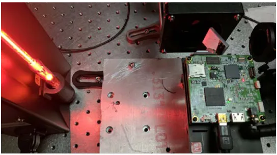
configuration is depicted in Fig. 7 (a). A Texas Instruments DLP LightCrafter Evaluation

Module is illuminated by a xenon arc lamp through a series of three mirrors (M1 through

25 the angular spectrum under measurement. Reflected light is then collimated by a

collimation lens (50 mm focal length) into a two-mirror (M4 and M5) FPE, which consists

of two 10:90 (R:T) dielectric plate beamsplitters from Thorlabs (BSN16) with reflectance

magnitudes of R1 and R2, respectively. Mirror M4 is placed on a translation stage, which

allows tuning the etalon’s thickness t. An objective lens (50 mm focal length) focuses the

FPE’s reflected light onto a ground glass diffuser and integrating rod, where the spatial

information is homogenized. Homogenization ensures both a uniform spatial and spectral

angular spectrum across the measured beam, which is often inhomogeneous due to

diffraction from the SLM. Finally, the light is measured by a spectrometer at the

homogenized output. A photo of the experimental setup is presented in Fig. 7 (b).

Fig. 7. (a) Schematic of the experimental configuration for the FPE-based interferometer; (b) photo of the setup on the benchtop.

The spectrometer that was implemented for measuring the channeled spectra is illustrated

in Fig. 8 (a). Light from the output fiber illuminates a 20 μm slit, which is then collimated

by a 50 mm focal length Nikon Nikkor F/1.8D lens. Collimated light from the slit