Blind Deconvolution with Model Discrepancies

Blind Deconvolution with Model Discrepancies

Dirisala Sumalatha (M.Tech Scolar)

& Sk.Ayesha (Asst Professor)

AMARA institute of engineering and technology,Guntur, Andhra Pradesh 522549, India1,2

[email protected]_{, [email protected]}2

A

BSTRACT

Blind deconvolution is a strongly ill-posed problem comprising of simultaneous blur and image estimation. Recent advances in prior modeling and/or inference methodology led to methods that started to perform reasonably well in real cases. However, as we show here, they tend to fail if the convolution model is violated even in a small part of the image. Methods based on variational Bayesian inference play a prominent role. In this paper, we use this inference in combination with the same prior for noise, image, and blur that belongs to the family of independent non-identical Gaussian distributions, known as the automatic relevance determination prior. We identify several important properties of this prior useful in blind deconvolution, namely, enforcing non-negativity of the blur kernel, favoring sharp images over blurred ones, and most importantly, handling non-Gaussian noise, which, as we demonstrate, is common in real scenarios. The presented method handles discrepancies in the convolution model, and thus extends applicability of blind deconvolution to real scenarios, such as photos blurred by camera motion and incorrect focus.

Index Terms— Blind deconvolution, variational bayes, automatic relevance determination, gaussian scale mixture.

I

.I

NTRODUCTION

Numerous measuring processes in real world are modeled by convolution. The linear operation of convolution is characterized by a convolution (blur) kernel, which is also called a point spread function (PSF), since the kernel is equivalent to an image the device would acquire after measuring an ideal point

source (delta function). In devices with classical optical systems, such as digital cameras,

Optical microscopes or telescopes, image blurs caused by camera lenses or camera motion is modeled by convolution. Media turbulence (e.g. atmosphere in the case of terrestrial telescopes) generates blurring that is also modeled by convolution. In atomic force microscopy or scanning tunneling microscopy, resulting images are convolved with a PSF, whose shape is related to the measuring tip shape. In medical imaging, e.g. magnetic resonance perfusion, pharmacokinetic models consist of convolution with an unknown arterial input function. These are just a few examples of acquisition processes with a convolution model. In many practical applications convolution kernels are unknown.

Then the problem of estimating latent Manuscript received data from blurred observations without any knowledge of kernels is called blind deconvolution. Due to widespread presence of convolution in images, blind deconvolution is an active field of research in image processing and computer vision. However, the convolution model may not hold over the whole image. Various optical aberrations alter images so that only the central part of images follows the convolution model. Physical phenomena such as occlusion, under and overexposure, violate the convolution model locally. It is therefore important to have a methodology that handles such discrepancies in the convolution model automatically.

𝑔 = ℎ ∗ 𝑢 + 𝜖 (1)

The goal of blind image deconvolution is to recover u solely from the given blurry image g. We follow the stochastic approach and all the variables in consideration are 2D random fields characterized by corresponding probability distributions denoted as p(h), p(u), and p(𝜖).

The Bayesian paradigm dictates that the inference of u and h from the observed image g is done by modeling the posterior probability distribution p(u, h|g) ∝ p(g|u, h)p(u)p(h). Estimating the pair (u ˆ, h ˆ) is then accomplished by maximizing the posterior p(u, h|g), which is commonly referred to as maximum a posteriori (MAP) approach, sometimes denoted MAP u,h to emphasize the simultaneous estimation of image and blur. Levin et al. in [1] pointed out that even for image priors p(u) that correctly capture natural image statistics (sparse distribution of gradients), MAPu,h approach tends to fail by returning a trivial ―no-blur‖ solution, i.e., the estimated sharp image is equal to the input blurred input g and the estimated blur is a delta function. However, MAP u,h avoids the ―no-blur‖ solution if we artificially sparsify intermediate images by shock filtering, removing weak edges, overestimating noise levels, etc., as widely used in [2]–[8].

From the Bayesian perspective, a more appropriate approach to blur kernel estimation is by maximizing the posterior marginalized w.r.t. the latent image u, i.e. p(h|g) = 𝑝(𝑢, ℎ/𝑔)𝑑𝑢. This distribution can be expressed in closed form only for simple image priors (e.g. Gaussian) and suitable approximation is necessary in other cases. In the Variational Bayesian (VB) inference, we approximate the posterior p(u, h|g) by a restricted parameterization in factorized form and optimize its Kullback-Leibler divergence to the correct solution. The optimization is tractable and the resulting approximation provides an estimate of the sought marginal distribution p(h|g). As soon as the blur h is estimated, the problem of recovering u becomes much easier. It can be usually determined by the very same model, only now we maximize the posterior p(u|g, h), or outsourced to any of the multitude of available non-blind deconvolution methods.

It is important to realize, that the error between the observation and the model, 𝜖 = g − h ∗ u, may not always be of stochastic uncorrelated zero-mean Gaussian nature – the true noise. In real-world cases, the observation error comes from many sources, e.g. sensor saturation, dead pixels or blur space-variance (objects moving in the scene) to name a few. Vast majority of blind deconvolution methods do not take any extra measures to handle model violation and the fragile nature of blind blur estimation typically causes complete failure when more than just a few pixels do not fit the assumed model, which unfortunately happens all too often. A non-identical Gaussian distribution with automatically estimated precision, which is called the Automatic Relevance Determination model (ARD) [9], is simple enough to be computationally tractable in the VB inference and yet flexible enough to handle model discrepancies far beyond the limited scope of Gaussian noise.

In this work, we adopt the probabilistic model of Tzikas et al. [10], which is based solely on VB approximation of the posterior p(u, h) and which uses the same ARD model for all the priors p(u), p(h), and importantly also for the noise distribution p(𝜖) . Our main focus is to analyze properties of the VB-ARD model and to elaborate on details of its implementation in real world scenarios, which was not directly considered in the original work of Tzikas. Specifically, we propose several extensions: include global precision for the whole image in the noise distribution p(𝜖.) to decouple the Gaussian and non-Gaussian part of noise, different approximation of the blur covariance matrix, pyramid scheme for the blur estimation, and handling convolution boundary conditions. We demonstrate that VB-ARD with proposed extensions is robust to outliers and in this respect outperforms by a wide margin state-of-the-art methods.

II.

L

ITERATURE

S

URVEY

[1] A. Levin, Y. Weiss, F. Durand, and W. T. Freeman, Blind deconvolution is the recovery of a sharp version of a blurred image when the blur kernel is unknown. Recent algorithms have afforded dramatic progress, yet many aspects of the problem remain challenging and hard to understand. The goal of this paper is to analyze and evaluate recent blind deconvolution algorithms both theoretically and experimentally. We explain the previously reported failure of the naive MAP approach by demonstrating that it mostly favors no-blur explanations. We show that, using reasonable image priors, a naive simulations MAP estimation of both latent image and blur kernel is guaranteed to fail even with infinitely large images sampled from the prior. On the other hand, we show that since the kernel size is often smaller than the image size, a MAP estimation of the kernel alone is well constrained and is guaranteed to succeed to recover the true blur. The plethora of recent deconvolution techniques makes an experimental evaluation on ground-truth data important. As a first step toward this experimental evaluation, we have collected blur data with ground truth and compared recent algorithms under equal settings. Additionally, our data demonstrate that the shift-invariant blur assumption made by most algorithms is often violated.

This paper analyzes the major building blocks of recent blind deconvolution algorithms. We illustrate the limitation of the simple MAPx;k approach, favoring the no-blur (delta kernel) explanation. One class of solutions involves explicit edge detection. A more principled strategy exploits the dimensionality asymmetry, and estimates MAPk while marginalizing over x. While the computational aspects involved with this marginalization are more challenging, existing approximations are powerful. We have collected motion blur data with ground truth and quantitatively compared existing algorithms. Our comparison suggests that the variational Bayes approximation [5] significantly outperforms all existing alternatives. The conclusions from our analysis are useful for directing future blind deconvolution research. In particular, we note that

modern natural image priors do not overcome the MAPx;k limitation (and in our tests did not change the observation in Section 2). While it is possible that blind deconvolution can benefit from future research on natural image statistics, this paper suggests that better estimators for existing priors may have more impact on future blind deconvolution algorithms. Additionally, we observed that the popular spatially uniform blur assumption is usually unrealistic. Thus, it seems that blur models which can relax this assumption have a high potential to improve blind deconvolution results.

[2] J. Pan, Z. Lin, Z. Su, and M. H. Yang, Estimating blur kernels from real world images is a challenging problem as the linear image formation assumption does not hold when significant outliers, such as saturated pixels and non-Gaussian noise, are present. While some existing non-blind deblurring algorithms can deal with outliers to a certain extent, few blind deblurring methods are developed to well estimate the blur kernels from the blurred images with outliers. In this paper, we present an algorithm to address this problem by exploiting reliable edges and removing outliers in the intermediate latent images, thereby estimating blur kernels robustly. We analyze the effects of outliers on kernel estimation and show that most state-of-the-art blind deblurring methods may recover delta kernels when blurred images contain significant outliers. We propose a robust energy function which describes the properties of outliers for the final latent image restoration. Furthermore, we show that the proposed algorithm can be applied to improve existing methods to deblur images with outliers. Extensive experiments on different kinds of challenging blurry images with significant amount of outliers demonstrate the proposed algorithm performs favorably against the state-of-the-art methods.

a robust method to restore the latent image under the guidance of the proposed outlier-aware function where the effects of outliers are minimized. Extensive experimental evaluations on real images and benchmark datasets demonstrate the proposed algorithm performs favorably against the state-of-the-art methods for uniform as well as non-uniform deblurring.

[3] W. Ren, X. Cao, J. Pan, X. Guo, W. Zuo, and M. H. Yang,Low rank matrix approximation has been successfully applied to numerous vision problems in recent years. In this paper, we propose a novel low rank prior for blind image deblurring. Our key observation is that directly applying a simple low rank model to a blurry input image significantly reduces blur even without using any kernel information, while preserving important edge information. The same model can be used to reduce blur in the gradient map of a blurry input. Based on these properties, we introduce an enhanced prior for image deblurring by combining the low rank prior of similar patches from both the blurry image and its gradient map. We employ a weighted nuclear norm minimization method to further enhance the effectiveness of low rank prior for image deblurring, by retaining the dominant edges and eliminating fine texture and slight edges in intermediate images, allowing for better kernel estimation. In addition, we evaluate the proposed enhanced low rank prior for both uniform and non-uniform deblurring. Quantitative and qualitative experimental evaluations demonstrate that the proposed algorithm performs favorably against the state-of-the-art deblurring methods.

In this paper, we present a novel enhanced low rank prior for blind image deblurring. The low rank properties of both intensity and gradient maps from image patches are exploited in the proposed algorithm. We present a weighted nuclear norm minimization approach based low rank properties to effectively recover latent images. Experimental results on benchmark datasets show that the proposed algorithm performs favorably against the state-of-the-art deblurring methods.

III.

P

ROPOSED

M

ETHOD

A.

A

R

D

In the discrete domain, convolution is expressed as matrix vector multiplication. Then according to (1) the data error 𝜖i of the i-th pixel is

𝜖i = gi − Hiu = gi − Ui h , i = 1,..., N , (2)

where H and U are convolution matrices performing convolution with the blur and latent image, respectively, and u are column vectors containing lexicographically ordered elements of the corresponding 2D random fields. N is the total number of pixels. Subscript i in vectors denotes the i-th element and in matrices i-the i-i-th row.

If the subscript is omitted then we mean the whole vector (or matrix). In the majority of blind deconvolution methods, the data error term is assumed to be i.i.d. zero-mean Gaussian with precision α, i.e.

𝑝 𝜖 𝛼 = 𝒩 𝜖_𝑖 0, 𝛼−1 𝑖

(3)

Such assumption leads to the common 2 data term α 2 i(gi − Uih)2. However as we demonstrate below, if this Gaussian error assumption is slightly violated (e.g. by pixel saturation, model locally doesn’t hold, etc.), the 2 data term gives an incorrect solution. It is therefore desirable to model both the Gaussian and non-Gaussian part of the error, for which the Student’s t-distribution is a good choice, as it is essentially a scaled mixture of Gaussians and also plays nicely with the VB framework.

As demonstrated earlier for the autoregressive model , we propose using a Gaussian distribution with pixel-dependent factors γi modulated by the overall noise precision α. The error model of is then defined as

𝑝 𝜖 𝛼, 𝛾 = 𝒩 𝜖𝑖 0, (𝛼𝛾𝑖)−1 𝑖

(4)

to which we refer as the ARD model with common precision. To draw a parallel to the classical formulation, the data term in this case takes the form

model lies in determining the precisions α and γi automatically. This is covered in the following section, where we formulate the VB inference. For the current discussion, it suffices to state that we need priors also on γ. Let G denote the standard Gamma distribution, defined as G (ξ|a, b) = (1/ (a)) baξia−1 exp (−bξ). We define the γ prior as

p 𝛾 𝑣 = 𝒢 𝛾_𝑖 𝑣 , 𝑣

𝑖

(5)

Marginalizing p (𝜖|α, γ )p(γ |ν) over γ gives us the Student’s t-distribution with zero mean, precision α and degrees of freedom 2ν. From the above model it follows that the mean of γi is equal to a/b = ν/ν = 1. If ν becomes large then G (γi|ν, ν) tends to the delta distribution at 1 and the error model will be just a Gaussian distribution. As ν decreases, tails decay more slowly and γi will be allowed to adjust and automatically suppress outliers violating the acquisition model. The conventional ARD model used e.g. in [10] is

𝑝∗ _{𝜖 𝛾 = 𝒩 𝜖} 𝑖 0, 𝛾𝑖−1 𝑖

𝑝∗ _𝛾

𝑖 = 𝒢 𝛾𝑖 𝑎𝛾, 𝑏𝛾 (6)

The marginal distribution of this prior over γ is a Student’s t-distribution with 2a γ degrees of freedom. It is possible to choose the number of degrees of freedom as a priori known – a common approach is to choose aγ, bγ as small as possible, yielding Student’s t-prior with infinite variance. Estimation of the hyper parameters aγ , bγ via a numerical MAP method has been proposed in [10].

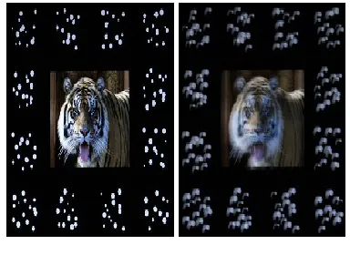
Fig.1. Sharp (left) and intentionally blurred (right) image pair acquired for accurate calculation of the blur PSF from the known patterns surrounding the image.

Fig. 2. Convolution error distribution in the case of real motion blurs (solid green).

It is much more heavy-tailed than the usually assumed Gaussian (dotted red, α = 0.6 · 103), while the Student’s t-distribution (dashed blue, 2ν = 3.5, α = 1.2 · 105) is a perfect fit.

The ARD model is valuable in real scenarios even when there are no visible local discrepancies of the convolutional model. We conjecture that under real image acquisition conditions there exists no convolution kernel h such that the distribution of in (2) is strictly Gaussian. Different factors inherently present in the acquisition process, such as lens imperfections, camera sensor discretization and quantization, contribute to the violation of the convolution model.

and plotted its distribution (negative log) in Fig. 2. The distribution is far from Gaussian, as the maximum likelihood estimate of the Gaussian distribution clearly provides a very poor approximation, especially in the tails. The Student’s t-distribution, on the other hand, approximates the error distribution correctly and thus justifies the ARD choice for p ().It is interesting to note, that we performed a similar analysis on Levin’s dataset [1] and obtained the same Student’s t-distribution of the convolution error. Another justification of the ARD model provided in [10]

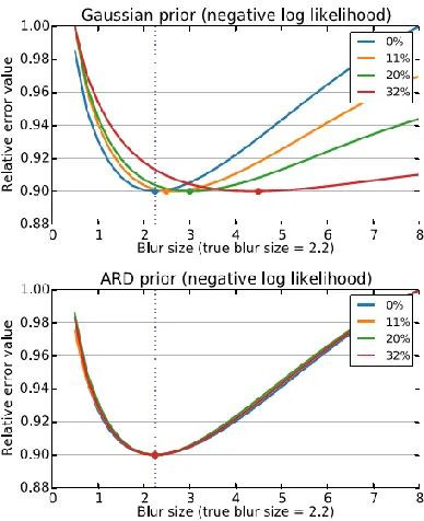
Fig.3. Relative data term value (negative log likelihood) for commonly used Gaussian (top) and ARD (bottom) priors (low value means high probability of the particular PSF) for image blurred with PSF of size 2.2.

Different data series correspond to different percentages of non-Gaussian error in the input. The curves’ minima (indicated by dots) should correspond to the true PSF (vertical line). The Gaussian prior favors larger and larger blurs as the non-Gaussian error increases, while the ARD prior remains virtually unaffected and correctly identifies the true PSF.

is that a small error in the blur estimation also produces heavy tailed p(). Having demonstrated that the model error may have a significantly non-Gaussian distribution, the logical next step is to further analyze how this influences the solution accuracy. We conducted an experiment to answer a question: Is the ubiquitous standard-issue quadratic data term (Gaussian model) the right choice in the presence of non-Gaussian input error? As one expects, the answer is no. The problem is that in the presence of non-Gaussian error, the quadratic data term attains its minimum at a wrong point, therefore we get a solution, however not the solution we sought. The setup of our experiment was as follows.

We took a sharp image u and set a certain percentage of randomly selected pixels to over-exposed values to represent non-Gaussian error. We then blurred the saturated image with the ―true‖ PSF ht, added mild Gaussian noise and clipped the image intensities to obtain the final image g. We then proceeded to measure the goodness of several PSF candidates h by evaluating the corresponding data terms (more precisely, − log (·) of the assumed noise distribution) of the classical Gaussian model (3) and the ARD model with common precision (4). The whole experiment is graphically documented in two plots in Fig. 3. The top plot corresponds to the Gaussian model (quadratic data term) and the bottom plot corresponds to the ARD model used by our method. Individual line series represent different percentage of pixels intentionally corrupted by non-Gaussian error.

error can be expected the Gaussian presents a poor choice for the likelihood, a choice which compromises the chances of successful sharp image restoration.

B.

V

B

I

There are many examples of the VB inference applied to blind deconvolution in the literature; see e.g. [10]. They approximate the posterior p(u, h|g) by a factorized distribution q(u, h) = q(u)q(h). We follow the same path and use the ARD model with common precision for the error and the conventional ARD model for image and blur priors. The common precision in the image and blur priors is in our opinion superfluous, since it lacks any relation to real phenomena as opposed to the error where the common precision models white Gaussian noise. Let us first define the individual distributions. Substituting from (2) into the ARD model in (4), the conditional probability distribution of the blurred image is

𝑝 𝑔 𝑢 , ℎ, 𝛼, 𝛾 = 𝒩 𝑔 𝐻 𝑢, 𝛼Γ−1

= 𝒩 𝑔_𝑖 𝐻𝑖𝑢, 𝛼𝛾𝑖 −1 𝑖

𝛼 (𝛼𝛾𝑖)1/2exp −

𝛼𝛾_𝑖

2 𝑔𝑖− 𝐻𝑖𝑢

2 _{, (7)}

where −1 is a diagonal covariance matrix having the inverse of the precision vector γ on the main diagonal, = diag(γ). Let us recall that the precision γi is in general different for every pixel and it is determined from the data, which allows for automatic detection and rejection of outliers violating the acquisition model. The image prior p (u) is defined over image features (derivatives) and takes the form

𝑝 𝑢 𝜆 = 𝒩 𝐷𝑢 0 ,Λ−1 _{= 𝒩(𝐷}

𝑖𝑢 0 , 𝜆𝑖−1) 𝑖

𝛼 𝜆1/2_𝑖 exp −𝜆𝑖 2(𝐷𝑖𝑢)

2

𝑖

, (8)

where Di is the first order difference at the i-th pixel and = diag (λ). The operator D can be replaced by any sparsifying image transform, like wavelet transform or other set of high pass filters. The prior

ability to capture sparse features (edges) comes from the automatically determined precisions λi’s. It was advocated in [1] to use flat priors on the blur and enforce only non-negativity, hi ≥ 0, and constant energy, i |hi| = 1. This reasoning stems from the fact that the blur size is by several orders of magnitudes smaller than the image size and therefore inferring the blur from the posterior is driven primarily by the likelihood function (7) and less by the prior p (h). However, if the image estimation u is inaccurate, which is typically the case in the initial stages of any blind deconvolution algorithm, then a more informative prior p (h) is likely to help in avoiding local maxima and/or speeding up the convergence. To keep the approach coherent, we apply the ARD model on blur intensities.

𝑝 ℎ 𝛽 = 𝒩 ℎ 0, 𝐵−1 _{= 𝒩 ℎ} 𝑖 0, 𝛽𝑖−1 𝑖

𝛼 𝛽_𝑖1 2

𝑖

exp −𝛽𝑖 2ℎ𝑖

2 ₍₉₎

where B = diag(β). The ARD models in (7), (8), and (9) are conditioned to unknown precision parameters (α, γi, λi, βi). The conjugate distributions of precisions are Gamma distributions and thus for image and blur precisions we have

𝑝 𝜆𝑖 = 𝒢 𝜆𝑖 𝑎𝜆, 𝑏𝜆

𝑝 𝛽_𝑖 = 𝒢 𝛽𝑖 𝑎𝛽, 𝑏𝛽 (10)

And for the error precisions according to (4) and (5) we have

𝑝 𝛼 = 𝒢 𝛼 𝑎_𝛼,𝑏_𝛼

𝑝 𝛾_𝑖 𝜈 = 𝒢 𝛾_𝑖 𝜈, 𝜈

𝑝 𝜈 = 𝒢 𝜈 𝑎_𝜈, 𝑏_𝜈 (11)

The hyper parameters a(·) and b(·) are user-defined constants. Let Z = {u, h, α, ν, {γi}, {λi}, {βi}} denote all the unknown variables and Zk its particular member indexed by k. Using the above defined distributions, the posterior p (Z|g) is proportional to

The VB inference [38] approximates the posterior p(Z|g) by the factorized distribution

𝑝 Ζ 𝑔 ≈ 𝑞 Ζ

= 𝑞 𝑢 𝑞 ℎ 𝑞 𝜈 𝑞 𝛾 𝑞 𝜆 𝑞 𝛽 (12)

This is done by minimizing the Kullback-Leibler divergence, which provides a solution for individual factors

𝑙𝑜𝑔𝑞 𝑧_𝑘 𝛼 𝔼𝑙≠𝑘 log 𝑝 Ζ 𝑔 (13)

where El=k denotes expectation with respect to all factors q (Zl) except q(Zk). Formula (13) gives implicit solution, because each factor q (Zk) depends on moments of other factors. We must therefore resort to an iterative procedure and update the factors q in a loop. A detailed derivation of update equations can be found in [10] as the model is similar to ours. The interested reader is also referred to [10] for better understanding of the derivation. In the following subsections we therefore only state the update equations yet analyze their properties in detail. A. Likelihood the important feature is automatic estimation of the nonGaussian part of the error modeled by precision γ. utilizing the combination of VB inference and ARD prior, we are able to detect and effectively reject outliers from the estimation and achieve unprecedented robustness of the blur estimation, much needed in practical applications. Using (13), q (γ) becomes a Gamma distribution with a mean value

γ_i = 1 + 2v

α 𝔼u,h[ gi− Hiu)2 + 2υ

(14)

where (·) denotes a mean value. Relating the inference to the classical minimization of energy function − log p (u, h|g), the precision γi corresponds to the weight of the i-th pixel in data fidelity term. The above equation shows that this weight is inversely proportional to the (expected) reconstruction error at that pixel (up to the relaxation by ν/α) and it is updated during iterations, as the image and blurs estimates change. This technique is similar to the method of iteratively reweighted least squares (IRLS), where the quadratic data terms are reweighted according to the error at the particular data point to achieve greater robustness to outliers,

but here it arises naturally as part of the VB framework. We demonstrate how the method behaves with respect to outliers in the experimental section. According to (14), the mean value of γ depends, apart from u and h, only on the mean values α and ν. Using again the VB inference formula (13), one can deduce that both q (α) and q (ν) are Gamma distributions with mean values

𝛼 = 𝑁 + 2𝑎𝛼 𝛾𝑖 𝔼_𝑢,ℎ[(𝑔_𝑖− 𝐻_𝑖𝑢2_] 𝑁

𝑖=1 + 2𝑏𝑎

(15)

𝜐 = 𝑁 + 2𝑎𝜐 2 𝑁 (𝛾𝑖 − 𝔼_𝛾𝑖[log 𝛾𝑖 ] − 1)

𝑖=1 + 2𝑏𝜐

(16)

Fig.4. Estimated noise precision as a function of iterations:

The Variational Bayesian algorithm updates the noise precision in every iteration. The curves depict its typical development for different image SNRs; 50dB through 10dB. The diamond markers show the fixed update using geometric progression αk = 1.5αk−1.

Stop when the correct α (corresponding to the true noise level) is reached, which is not determined automatically but must be specified by the user. The VB framework has an indisputable advantage over more straightforward MAP methods – not only does it give us the optimal update equation for the data term precision, it also provides automatic saturation when the correct noise level is reached, as we can see in Fig. 4. During the early iterations the precision sharply increases and then levels out at the correct value. For comparison we also show the fixed geometric progression for r = 1.5 (diamond markers).

C.

I

P

The factors associated with the image are q (u) and q (λ). Applying (13), we get (up to a constant) log

𝑙𝑜𝑔𝑞 𝑢 = −Εℎ,𝛼,𝛾,𝜆 𝛼 𝑔 − 𝐻𝑢 𝑇Γ 𝑔 − 𝐻𝑢

+ 𝑢𝑇_𝐷𝑇_{Λ𝐷𝑢 (17)}

where the terms independent of u are omitted. The distribution q (u) is a normal distribution. The mean u and covariance cov (u) are obtained by taking the first and second order derivatives of log(q(u)), respectively, and solving for zero. The update equation for the mean is a linear system

𝔼h 𝐻𝑇Γ 𝐻 + 𝛼 −1𝐷𝑇Λ 𝐷 𝑢 =Η

𝑇_{Γ 𝑔 (18)}

And for the covariance we get

cov u = (𝛼 𝔼ℎ 𝐻𝑇Γ 𝐻 + 𝐷𝑇Λ 𝐷)−1 (19)

The mean pixel precisions λi form the diagonal matrix. They are calculated from q(λ), which is a Gamma distribution with the mean

λ_i= 1 + 2aλ 𝔼_u (Diu)2 + 2bλ

(20)

The parameter bλ plays the role of relaxation, as it prevents division by zero in the case Diu = 0.

Fig.5. Comparison of priors: The graph shows − log p(u) of priors as a function of amount of blurring.

The 1 prior (dotted red line) decreases and so does the log prior (dash-dotted yellow line), which is the marginalized ARD prior. On the other hand, the ARD prior (solid purple line) with precisions estimated from the sharp image steeply increases and flattens out for large blurs. The normalized prior 2 (dashed blue line) increases more slowly but steadily. The value of priors are normalized to give 1 on sharp images (1 blur size). The curves show means values calculated on various images (photos of nature, human faces, and buildings).

analyze if the ARD image prior p (u|λ) in (8) behaves better in this respect and how it compares with the unconditional (marginalized) version p (u). Following the analysis of Gaussian scale mixtures in [27] and [29], the unconditional prior p (u) is obtained by marginalizing over λ, which in the limit for aλ → 0 yields.

𝑝 𝑢

= 𝑝 𝑢, 𝜆 𝑑𝜆

= 𝑝 𝑢 𝜇 𝑝 𝜆 𝑑𝜆𝛼 exp⁡(−1

2log⁡((𝐷𝑖𝑢)

2

𝑖

+ 𝑏)) (21)

The marginalized ARD image prior is of the exponential form with exponent log (Di u)2 + const. It is thus equivalent to the log prior proposed in [22]. It is a non-convex prior that aggressively favors sparsity of the natural image statistics. In this sense it resembles the p priors with p → 0. We calculated − log p (u) on natural images (photos of nature, human faces, and buildings) blurred with Gaussian blur of varying size. We also tried motion and uniform blur and the behavior was identical. For each image we have normalized − log p (u) calculated on differently blurred versions of the image so the original sharp image (no blur) gives 1. The normalized − log p (u) of different priors as a function of blur size and averaged over all images is plotted in Fig. 5. As expected, the exponent of the 1 prior decrease as the blur increases, i.e. this prior favors blurred images over sharp ones. The log prior, which is the marginalized ARD prior, decreases less but still favors blurred images. In the VB framework, however, we do not work with the marginalized ARD prior and instead iteratively estimate the prior precisions λi’s from the current estimate of u using the update formula (20).

Let us assume an ideal situation in which the precisions are estimated from the sharp image, then the ARD prior shows correct behavior similarly to the normalized prior 2 [39] that compensates for the effect of decreasing image variance. This ideal case is not achievable in practice, since we do not have a correct estimate of the sharp image u at the beginning, but it can be regarded as an upper bound.

As the VB inference makes the approximation of the posterior more accurate with every iteration, we approach this upper bound.

D.

B

P

As stated earlier, we use the same ARD model also for the blur prior (9). Analogously to the derivation of the image distribution q(u) in (17), the form of blur factor q(h) is a Gaussian distribution given by log q(h) = −Eu,α,γ,β α(g − Uh)T (g − Uh) + hT Bh . Then the mean h is the solution of the linear system

𝔼 𝑈𝑇_{Γ 𝑈 + 𝛼} −1_{𝐵 ℎ = 𝑈}𝑇_{Γ 𝑔 (22)}

And the covariance is

𝑐𝑜𝑣 ℎ = (𝛼 𝔼_𝑢 𝑈𝑇_{Γ 𝑈 + 𝐵 )}−1 ₍₂₃₎

The distribution q (β) of the blur precision is again a Gamma distribution and for the mean values of βi we get analogously to (20)

𝛽 =𝑖

1 + 2𝑎_𝛽 𝔼_ℎ ℎ_𝑖2 _{+ 2𝑏}

𝛽

(24)

State-of-the-art blind deconvolution methods often estimate h while enforcing positivity and constant energy, i.e. hi ≥ 0 and i hi = 1. Enforcing such constraints in our case means to solve the least squares objective associated with (22) under these constraints. Since the constraints form a convex set, we can use, e.g., the alternating direction method of multipliers (ADMM) [40], that solves convex optimization problems by breaking them into smaller pieces, each of which is then easier to handle. However, applying such constraints would take us outside the VB framework, as q (h) is then no longer a Gaussian distribution and cov h is intractable.

typically initialized with delta functions. If during VB iterations, any hi approaches zero then the corresponding precision calculated in (24) grows, reaching 1/ (2b) if a → 0. If the hyper parameters are sufficiently small (which is our case), this correspond to a very tight distribution q(hi) that traps hi at zero and prevents further changes.

The covariance cov h has an additional positive influence on the behavior of the PSF precision β. The denominator of (24) expands to h2 i + cov hi + 2b. From (23) it follows that cov hi is inversely proportional to α + βi. We can ignore γ, since it is in average around 1 anyway as it captures only local nonGaussian errors. We have seen in Fig. 4 that α starts small, which implies larger cov hi and thus small PSF precision βi. Small βi loosely constrains the estimation of the PSF h during initial iterations. As α increase later on, cov hi decreases and βi increases, which helps to fix the estimated values of h.

E.

A

All equations in the VB inference are relatively easy to solve, except for the calculation of covariance matrices cov u in (19) and cov h in (23), which involves inverting precision (concentration) matrices. Both matrices are large and their inversion is not tractable since they are a combination of convolution and diagonal matrices. The covariance is important in the evaluation of expectation terms E [·]. To tackle this problem, we approximate precision matrices by diagonal ones. This is different from Tzikas’s work [10], where cov h is approximated by a convolution matrix. The experimental section demonstrates that the diagonal approximation performs better. We show the approximation procedure on cov h and calculation of u. The approximation of cov u and calculation of h is similar. First we approximate the covariance matrix cov h by inverting only the main diagonal of the precision matrix, i.e.,

(Diag (αEu U T U + B))−1.

Here we use the syntax of popular numerical computing tools such as MATLAB, Python or R, and assume that the operator diag (·) if applied to a

matrix returns its main diagonal. The covariance cov h is required in the evaluation of Eh H T H in (18). After some algebraic manipulation, we conclude that Eh H T H = H T H +Ch, where Ch is a diagonal matrix constructed by convolving γ with cov h. We can interpret the main diagonals of cov h and as 2D images and then by slightly abusing the notation write Ch = diag γ ∗ (diag(αU T U + Cu + B))−1, where the outer operator diag(·) returns a diagonal matrix with pixels of the convolution result arranged on the main diagonal. The blind deconvolution algorithm is summarized in Algorithm 1.

Algorithm 1 The estimated blur h is then upsampled and used as an initialization in the next run of the algorithm with the corresponding scale of g. This is repeated until the original scale of g is reached. We tested various configurations and concluded that 5 scales with a scale factor of 1.5 is sufficient, which was then used in all our experiments. Passing other variables (e.g. precisions) between scales except h proved superfluous. The second point is to handle convolution boundary conditions, which is necessary in the case of real images. We solve it naturally by forcing precisions γi’s that lie along image boundaries to zero.

This way the algorithm assumes maximal model discrepancy and completely ignores the boundary regions. The hyper parameters a (·) and b (·) in (10) and (11) are the only user-defined parameters. Checking update equations (15) and (16) reveals that (aα, bα) and (aν, bν) have a negligible effect since both α and ν are scalars and data terms in the update equations are dominant. In all our experiments we set them thus to zero. On the other hand, (aλ, bλ) and (aβ, bβ) are important since both λ and β are calculated for every pixel and their update equations (20) and (24) are influenced by the hyper parameters.

We have searched for the best parameters and determined that both aλ and aβ can be set to zero but bλ and bβ must be in the interval (10−9, 10−6), otherwise the algorithm is unstable. In the case of the noise model with conventional ARD, α and ν (and corresponding hyper parameters aα, bα, aν, bν) are not present. Instead, we have new hyper parameters aγ, bγ, which we set in all our experiments to 0 and 10−4, respectively. This corresponds to fixing the number of degrees of freedom to zero.

IV

E

XPERIMENTAL

R

ESULTS

Fig1: (a) Original Image (b) Synthetic Blur Image

Fig2: (a) Original Image (b) Blurred Image (c) Distorted Image (d) Restored Image

We considered distortion by 1) small regions 2) large regions 3) Gaussian large regions

Fig4: Original images and PSFs used in our synthetic experiments.

V

.C

ONCLUSIONS

We have presented a blind deconvolution algorithm using the Variational Bayesian approximation with the Automatic Relevance Determination model on likelihood and image and blur priors. The derived coherent algorithm consists of two linear systems of equations that can be efficiently solved with the Conjugate Gradients method, and three simple pixel wise update equations for noise, image and blur precisions. We have shown that the Automatic Relevance Determination model correctly favors sharp images over the blurred ones, enforces PSF non-negativity and most importantly adjusts for convolution model discrepancies. The experimental section has demonstrated that allowing variable data precision is essential for dealing with outliers such as saturated regions, occlusions or convolution boundary effects. Estimation of the degrees of freedom of the noise prior is beneficial only for Gaussian noise. For non-Gaussian noise distributions, it is more effective to fix the number of degrees of freedom to zero.

R

EFERENCES

[1] A. Levin, Y. Weiss, F. Durand, and W. T. Freeman, ―Understanding blind deconvolution algorithms,‖ IEEE Trans. Pattern Anal. Mach. Intell., vol. 33, no. 12, pp. 2354–2367, Dec. 2011. [2] J. Pan, Z. Lin, Z. Su, and M. H. Yang, ―Robust kernel

estimation with outliers handling for image deblurring,‖ in Proc. IEEE Conf. Comput. Vis. Pattern Recognit. (CVPR), Jun. 2016, pp. 2800– 2808.

[3] W. Ren, X. Cao, J. Pan, X. Guo, W. Zuo, and M. H. Yang, ―Image deblurring via enhanced low-rank prior,‖ IEEE Trans. Image Process., vol. 25, no. 7, pp. 3426–3437, Jul. 2016.

[4] L. Xu, S. Zheng, and J. Jia, ―Unnatural L0 sparse representation for natural image deblurring,‖ in Proc. IEEE Conf. Comput. Vis. Pattern Recognit. (CVPR), Jun. 2013, pp. 1107–1114. [Online].

[5] L. Zhong, S. Cho, D. Metaxas, S. Paris, and J. Wang, ―Handling noise in single image deblurring using directional filters,‖ in Proc. IEEE CVPR, Jun. 2013, pp. 612–619.

[6] L. Xu and J. Jia, ―Two-phase kernel estimation for robust motion deblurring,‖ in Proc. 11th Eur. Conf. Comput. Vis. (ECCV), Berlin, Germany, 2010, pp. 157–170.

[7] M. S. C. Almeida and L. B. Almeida, ―Blind and semi-blind deblurring of natural images,‖ IEEE Trans. Image Process., vol. 19, no. 1, pp. 36–52, Jan. 2010.

[8] S. Cho and S. Lee, ―Fast motion deblurring,‖ ACM Trans. Graph., vol. 28, no. 5, 2009, Art. no. 145.