Solution structure of macromolecules using
small angle neutron scattering and molecular
simulations
Jayesh S. Bhatt1,*
1University College London, Gower Street, London WC1E 6BT, UK
Abstract. An introductory account of using molecular simulations to
deduce solution structure of macromolecules using small angle neutron scattering data is presented for biologists. The presence of a liquid solution provides mobility to the molecules, making it difficult to pin down their structure. Here a simple introduction to molecular dynamics and Monte Carlo techniques is followed by a recipe to use the output of the simulations along with the scattering data in order to infer the structure of macromolecules when they are placed in a liquid solution. Some practical issues to be watched for are also highlighted.
1 Introduction
Biological macromolecules tend to have a high degree of flexibility and under physiological conditions, they are usually found within a liquid solution. In such an environment, the macromolecules undergo various types of motion continuously. Excellent progress has been made in crystallography to capture the atomistically detailed structures of molecules in the solid state. However, crystallographic structures may not accurately resemble those that are found in solution, nor do they provide information about the dynamics of the molecule under realistic physiological conditions. Since the molecules are moving in solution, it is difficult to obtain an atomistically detailed ‘snapshot’ experimentally. Instead, one can obtain orientationally averaged scattering data of the macromolecules in solution and then use computationally generated, physically plausible models of the macromolecule in order to deduce the structure and dynamics of the actual molecules.
Many different techniques are available for simulating the dynamics involving soft materials and the particular choice depends on the level of detail required and the amount of computational power at the user’s disposal. For instance, quantum mechanical methods, such as density functional theory, consider details down to the level of electron clouds within the individual atoms making up a molecule. This makes quantum mechanical techniques computationally demanding and very slow for large molecules. In macromolecules, where such precision is rarely required, techniques based on classical laws of physics are better suited in order to ensure that a sufficiently large range of molecular configurations are explored within a manageable computational time. This introduces the concept of coarse
graining in simulations. As the smallest unit of the material being simulated gets larger, the system is referred to as coarse-grained.
This chapter aims to provide a simplified introduction for biologists to two widely used techniques for computationally simulating the structure and dynamics of biological macromolecules under realistic interactions and constraints. In Sections 2 and 3 we go through the theoretical background behind the techniques of molecular dynamics (MD) and Monte Carlo (MC) simulations. After enlisting some of the issues and pitfalls that may arise in the simulations and possible ways to avoid them in Section 4, a typical workflow involved in using small angle neutron scattering (SANS) data to deduce solution structure of biological macromolecules is discussed in Section 5.
2 Molecular dynamics basics
When two atoms are placed close to each other, such as is the case in a molecule, they would, in general, exert mutual forces on each other. This is essentially due to the fact that atoms are not solid spheres with hard boundaries, but are enveloped by rather fuzzy probability clouds of negatively charged electrons that fade away gradually as one moves away from the centre of an atom. If the value of this mutual force, F, is known, one can solve the two simultaneous equations, one for each atom, resulting from Newton’s second law of motion:
𝐅𝐅 = 𝑚𝑚!𝐚𝐚!
−𝐅𝐅 = 𝑚𝑚"𝐚𝐚" ,
(1)
where𝑚𝑚!and𝑚𝑚"are the masses of the two atoms and𝐚𝐚!and 𝐚𝐚"are the accelerations of the
two atoms that result from this equal and opposite force acting on each other. Since an exact mathematical solution for 𝐚𝐚!and 𝐚𝐚"can be obtained in this way, the system is known as
analytically solvable and we can recreate and predict the positions of the two atoms in three-dimensional space as a function of time. If, however, one adds just one more atom to the system, it turns out that the resultant three simultaneous equations of motion cannot be solved analytically. Indeed, for a molecule with a large number of atoms, this becomes an N-body problem, which has no analytical solution and must be solved numerically with the help of a computer.
In a classical molecular dynamics simulation, trajectories of atoms and molecules are obtained in real time and space by numerically solving the appropriate (and usually large) set of time-dependent equations of motion. It is known as a deterministic technique, since the state of the system at a given time step can be predicted using the knowledge of the state of the system at the previous time step, provided that the time step is adequately small and that information about the manner in which the atoms (or ions) interact with each other is available. MD is widely used to understand the structure, dynamics, phase transformation and surface phenomena in soft matter and hard matter systems. MD simulations that incorporate the principles of quantum mechanics, instead of Newtonian mechanics, also exist; however, for macromolecules these are prohibitively expensive in terms of their execution time with the current generation of computers. Hence, we focus our discussion on classical MD.
2.1 Trajectory calculation
Assuming that the total force 𝐅𝐅%acting on each of the atoms𝑗𝑗 = {1, … , 𝑁𝑁}, where𝑁𝑁is the
graining in simulations. As the smallest unit of the material being simulated gets larger, the system is referred to as coarse-grained.
This chapter aims to provide a simplified introduction for biologists to two widely used techniques for computationally simulating the structure and dynamics of biological macromolecules under realistic interactions and constraints. In Sections 2 and 3 we go through the theoretical background behind the techniques of molecular dynamics (MD) and Monte Carlo (MC) simulations. After enlisting some of the issues and pitfalls that may arise in the simulations and possible ways to avoid them in Section 4, a typical workflow involved in using small angle neutron scattering (SANS) data to deduce solution structure of biological macromolecules is discussed in Section 5.
2 Molecular dynamics basics
When two atoms are placed close to each other, such as is the case in a molecule, they would, in general, exert mutual forces on each other. This is essentially due to the fact that atoms are not solid spheres with hard boundaries, but are enveloped by rather fuzzy probability clouds of negatively charged electrons that fade away gradually as one moves away from the centre of an atom. If the value of this mutual force, F, is known, one can solve the two simultaneous equations, one for each atom, resulting from Newton’s second law of motion:
𝐅𝐅 = 𝑚𝑚!𝐚𝐚!
−𝐅𝐅 = 𝑚𝑚"𝐚𝐚" ,
(1)
where𝑚𝑚!and𝑚𝑚"are the masses of the two atoms and𝐚𝐚!and 𝐚𝐚"are the accelerations of the
two atoms that result from this equal and opposite force acting on each other. Since an exact mathematical solution for 𝐚𝐚! and 𝐚𝐚" can be obtained in this way, the system is known as
analytically solvable and we can recreate and predict the positions of the two atoms in three-dimensional space as a function of time. If, however, one adds just one more atom to the system, it turns out that the resultant three simultaneous equations of motion cannot be solved analytically. Indeed, for a molecule with a large number of atoms, this becomes an N-body problem, which has no analytical solution and must be solved numerically with the help of a computer.
In a classical molecular dynamics simulation, trajectories of atoms and molecules are obtained in real time and space by numerically solving the appropriate (and usually large) set of time-dependent equations of motion. It is known as a deterministic technique, since the state of the system at a given time step can be predicted using the knowledge of the state of the system at the previous time step, provided that the time step is adequately small and that information about the manner in which the atoms (or ions) interact with each other is available. MD is widely used to understand the structure, dynamics, phase transformation and surface phenomena in soft matter and hard matter systems. MD simulations that incorporate the principles of quantum mechanics, instead of Newtonian mechanics, also exist; however, for macromolecules these are prohibitively expensive in terms of their execution time with the current generation of computers. Hence, we focus our discussion on classical MD.
2.1 Trajectory calculation
Assuming that the total force 𝐅𝐅% acting on each of the atoms𝑗𝑗 = {1, … , 𝑁𝑁}, where𝑁𝑁is the
number of atoms in the system, is known, a common numerical scheme to obtain the positions
of all the atoms at successive time steps is the Verlet algorithm [1]. It is derived by Taylor expanding the position 𝐫𝐫&(𝑡𝑡)up to third order in both forward and reverse time and then
adding the resulting two expressions. The end result is
𝐫𝐫&(𝑡𝑡 + Δ𝑡𝑡) = 2𝐫𝐫&(𝑡𝑡) − 𝐫𝐫&(𝑡𝑡 − Δ𝑡𝑡) +𝐅𝐅&𝑚𝑚(𝑡𝑡) & (Δ𝑡𝑡)
" (2)
which allows for the atomic positions to be calculated at time 𝑡𝑡 + Δ𝑡𝑡given the positions at times 𝑡𝑡and 𝑡𝑡 − Δ𝑡𝑡. In other words, it allows one to numerically propagate the trajectory forward in time using an existing set of atomic coordinates and forces. Other more sophisticated methods, such as the leapfrog algorithm, also exist [2].
The utility of Eq. (2) is conditional upon the time stepΔ𝑡𝑡being adequately small. As a rule of thumb, it should be smaller than the timescale of the fastest mode of movement present in the given system, e.g. the thermal vibrations of the atoms making up a molecule, in order to be able to capture the dynamics. Under room temperature and pressure conditions, atoms in a molecule typically vibrate at frequencies of10!'− 10!(Hz, which means a time step
of a few femtoseconds (10)!* s) would work without the simulation crashing. A time step
smaller that this would slow down the simulation unnecessarily without much gain in the accuracy of the results.
2.2 Force fields
The force 𝐅𝐅 appearing in Eq. (1) is derived from the interatomic interactions that are acting among the atoms (and ions) in the molecule. Naturally, defining these interactions accurately is the most crucial part of an MD simulation, as the level of accuracy in these dictates the trustworthiness of the evolution and the emergent structure of the molecule. Let us therefore take a qualitative overview of what constitutes a typical set of interatomic interactions, also known as the force field, that go into an MD simulation.
An interaction between two atoms labelled 𝑖𝑖 and 𝑗𝑗 is defined in terms of the interatomic potential energy, 𝑈𝑈(𝑟𝑟&%), that exists between these two atoms solely. The force experienced by atom 𝑗𝑗, 𝐅𝐅%, as a result of atom 𝑖𝑖 is related to the pair-potential energy 𝑈𝑈(𝑟𝑟&%) through the relation
𝐅𝐅% = −𝑟𝑟1 &%9
∂𝑈𝑈;𝑟𝑟&%<
∂𝑟𝑟&% = 𝐫𝐫&%,
(3)
where 𝐫𝐫&and𝐫𝐫%are the Cartesian coordinates of the two atoms with respect to an arbitrarily
defined origin in the simulation cell, while
𝐫𝐫&%= 𝐫𝐫% − 𝐫𝐫& (4)
is the vector from the 𝑗𝑗th atom to the 𝑖𝑖th atom and 𝑟𝑟
&%= >𝐫𝐫&%> is the scalar magnitude of this
vector. The function 𝑈𝑈(𝑟𝑟&%) is, somewhat confusingly, often referred to as simply potential
in the MD community. For the purpose of tractability, it is usually split into different parts that describe the various components of the overall interaction.
As a first split, the total potential energy, 𝑈𝑈Total, is expressed as a sum of the potential
energy due to chemical bonds, 𝑈𝑈Bonded, and the potential energy between chemically non-bonded atoms, 𝑈𝑈Non-bonded:
The term 𝑈𝑈Bonded can be further split as
𝑈𝑈Bonded= 𝑈𝑈Stretching+ 𝑈𝑈Bending+ 𝑈𝑈Torsion+ 𝑈𝑈Improper, (6)
where 𝑈𝑈Stretching represents the stretching motion between two chemically bonded atoms,
𝑈𝑈Bendingdescribes the bending of the bonds among three atoms, 𝑈𝑈Torsionis the dihedral angle
potential to allow for the twisting movement among atoms and 𝑈𝑈Improperrepresents dihedral potentials that are often used to restrict the geometry of molecules (e.g., to maintain the planar geometry of a molecule). Each of these four terms are harmonic in nature (i.e. an oscillating pattern around a mean central position). However, one could impose a rigid bond if required by replacing a given term with a constraint.
Non-bonded interactions are expressed as a sum of the electrostatic and van der Waals interactions:
𝑈𝑈Non-bonded= 𝑈𝑈Electrostatic+ 𝑈𝑈van-der-Waals. (7)
Here, 𝑈𝑈Electrostatic is the energy due to the Coulombic interaction between two electrical
charges, while 𝑈𝑈van-der-Waals takes into account dipole formation and the overlap of the electron
clouds of two (or more) atoms. The van der Waals component of the interaction is very important, since it ensures that two ions with opposite charges placed close to each other do not end up sitting on top of each other, as would happen if only the electrostatic interaction were to be present. A considerable amount of effort usually goes into determining the exact form of this part of the interaction as it also dictates the equilibrium distance between two atoms (or ions).
One popular form that is chosen to represent the van der Waals interaction is the Lennard-Jones (L-J) potential, also sometimes referred to as 6-12 or 12-6 potential. Its functional form is:
𝑈𝑈L-J;𝑟𝑟&%< = 4𝜖𝜖 BC𝑟𝑟𝜎𝜎 &%E
!"
− C𝑟𝑟𝜎𝜎
&%E F
F (8)
To understand this potential, it is useful to sketch the magnitude of 𝑈𝑈L-J as a function of the interatomic distance, 𝑟𝑟&%, as shown in Figure 1. The parameter 𝜖𝜖 is the ‘depth’ of the L-J
potential energy and is equal to the minimum energy required to break the van der Waals bond between atoms 𝑖𝑖 and 𝑗𝑗, while 𝜎𝜎 is the interatomic finite distance at which the L-J potential energy is zero. Since the interatomic force is defined in terms of the slope of the potential energy, the minimum of the curve in Figure 1, marked by a red dot, represents the equilibrium point where the slope, and hence the interatomic force, is zero. The part of the curve to the left of this point represents repulsive force between the atoms, which in the real world occurs due to the overlap of the electron clouds of the atoms, while the part to the right characterises attractive force. Hence, this form of the potential is a convenient way of mimicking the spring-like character of the forces that exist between neutral atoms in the real world: when two atoms are pulled apart away from the equilibrium distance, they will tend to attract each other; however, if the two atoms come closer to each other than the equilibrium distance, they would experience a rapidly increasing repulsive force that will ensure that the two atoms do not quite merge into each other and will move away quickly. It also follows that at a non-zero finite temperature, two atoms placed close to each other will thus tend to perform oscillatory motion about the equilibrium point.
To obtain the value of the equilibrium distance 𝑟𝑟GH, one can evaluate the first derivative of Eq. (8) with respect to 𝑟𝑟&% and equate it to zero. This leads to
𝑟𝑟GH= 2!/F𝜎𝜎 (9)
Equation (8) can therefore be rewritten as
𝑈𝑈L-J;𝑟𝑟&%< = 𝜖𝜖 BC𝑟𝑟𝑟𝑟GH &%E
!"
− 2 C𝑟𝑟𝑟𝑟GH
&%E F
F. (10)
In literature, both these forms of 𝑈𝑈L-J;𝑟𝑟&%< can be found since both of them are equivalent. In
a typical MD software, only the numerical values of 𝜖𝜖, in addition to 𝜎𝜎 or 𝑟𝑟GH, depending on whether Eq. (8) or (10) is implemented in the software, need to be provided while defining the L-J potential.
Another parameter that requires to be specified in an MD simulation is the cut-off distance, 𝑟𝑟JKL. This is the distance from a given atom when both the potential energy and the
interatomic force are assumed to have fallen to negligible values. In Figure 1 it can be seen that at 𝑟𝑟&%= 𝑟𝑟JKL not only 𝑈𝑈L-J;𝑟𝑟&%< is very close to zero, the slope of the curve is also very
small, making the force negligible according to Eq. (3). Hence, considering interactions beyond this radius of influence would be a waste of computational effort. It is therefore necessary to choose this distance wisely. A large value of 𝑟𝑟JKL may slow down the simulation
unnecessarily without perceptible gain in the accuracy of the results, while choosing too small a value would risk sacrificing the accuracy. For biomolecular simulations, 𝑟𝑟JKL≈ 15 Å is
usually adequate, although values as small as 10 Å are not uncommon in literature.
Fig. 1: Lennard-Jones interaction curve between two non-bonded atoms. The red dot marks the point of equilibrium between the two atoms.
well-known biomolecular potentials include AMBER [3], BMS [4], CHARMM [5], ECEPP [6], GROMOS [7-9], MM3 [10], OPLS [11] and PFF [12], although this list is by no means exhaustive.
Some of the popular, freely available MD packages include DL_POLY [13], NAMD [14], GROMACS [15], CHARMM [16] and LAMMPS [17]. Each of these packages have their own appeal and individuals’ choice is often based on the exact nature of the system to be simulated.
3 Monte Carlo approach
While MD is a deterministic technique, whereby the positions of the atoms evolve in a sequential manner from one time step to another following the laws of mechanics, Monte Carlo is known as a stochastic or non-deterministic technique. In MC, the state of the system from one step to another evolves in a random manner, albeit within physical constraints imposed by factors such as chemical bonds, force fields, temperature, pressure and so forth. Not all of these constraints need to be imposed in a particular simulation and this is something to be decided by the software designers and the users.
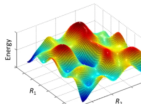
In order to understand how a molecular system can be probed through random means, one needs to first consider the concept of potentialenergy surface in physics, which, contrary to the common meaning of the word ‘surface’, could in general be a 𝑛𝑛-dimensional entity, where 𝑛𝑛 is the number of degrees of freedom present in the system. Figure 1 is an example of an energy curve with only one degree of freedom, namely the distance between two atoms. In Figure 2, an energy surface with two degrees of freedom, denoted as𝑅𝑅!and𝑅𝑅", is shown
known biomolecular potentials include AMBER [3], BMS [4], CHARMM [5], ECEPP [6], GROMOS [7-9], MM3 [10], OPLS [11] and PFF [12], although this list is by no means exhaustive.
Some of the popular, freely available MD packages include DL_POLY [13], NAMD [14], GROMACS [15], CHARMM [16] and LAMMPS [17]. Each of these packages have their own appeal and individuals’ choice is often based on the exact nature of the system to be simulated.
3 Monte Carlo approach
While MD is a deterministic technique, whereby the positions of the atoms evolve in a sequential manner from one time step to another following the laws of mechanics, Monte Carlo is known as a stochastic or non-deterministic technique. In MC, the state of the system from one step to another evolves in a random manner, albeit within physical constraints imposed by factors such as chemical bonds, force fields, temperature, pressure and so forth. Not all of these constraints need to be imposed in a particular simulation and this is something to be decided by the software designers and the users.
In order to understand how a molecular system can be probed through random means, one needs to first consider the concept of potentialenergy surface in physics, which, contrary to the common meaning of the word ‘surface’, could in general be a 𝑛𝑛-dimensional entity, where 𝑛𝑛 is the number of degrees of freedom present in the system. Figure 1 is an example of an energy curve with only one degree of freedom, namely the distance between two atoms. In Figure 2, an energy surface with two degrees of freedom, denoted as𝑅𝑅!and𝑅𝑅", is shown
(it would be impossible to graphically depict an energy surface with three or more degrees of freedom). It consists of hills, valleys and saddle points. Each minimum within a given valley is known as a local minimum, while the absolute lowest point within the entire surface is known as the global minimum. This kind of shape of the energy surface is generally caused as a result of the competing forces that an atom experiences from different directions. Since the atoms are constantly trying to minimise their own energy, one would expect theatoms to spend most of the time in regions around the local minima. Excursion onto higher energy points occurs as a result of temperature, which drives thermal fluctuations, which occasionally also leads to an atom climbing all the way up a hill and dropping into a neighbouring local minimum. Clearly then, the higher the energy, the lower the probability of finding atoms in that energy state and vice versa.
Fig. 2: Typical energy surface of a system with two degrees of freedom, labelled as𝑅𝑅!and𝑅𝑅".
It is this key observation that is utilised cleverly in a Monte Carlo simulation involving molecular structure. If 𝐪𝐪and𝐩𝐩are two large vectors specifying the instantaneous positions and momenta, respectively, of all the atoms in the system, i.e.
𝐪𝐪 = (𝑥𝑥!, 𝑦𝑦!, 𝑧𝑧!, 𝑥𝑥", 𝑦𝑦", 𝑧𝑧", … , 𝑥𝑥M, 𝑦𝑦M, 𝑧𝑧M) (11)
𝐩𝐩 = (𝑝𝑝N,!, 𝑝𝑝O,!, 𝑝𝑝P,!, 𝑝𝑝N,", 𝑝𝑝O,", 𝑝𝑝P,", … , 𝑝𝑝N,M, 𝑝𝑝O,M, 𝑝𝑝P,M), (12)
then the space containing all the possible combinations of (𝐪𝐪, 𝐩𝐩) is known as the phase space of the given system. The phase space contains all the information that is necessary to describe the state of the system. The probability 𝑃𝑃(𝐪𝐪, 𝐩𝐩)of finding the system at a particular phase point is connected with the system energy, 𝐸𝐸(𝐪𝐪, 𝐩𝐩) through the equation
𝑃𝑃(𝐪𝐪, 𝐩𝐩) = 𝑍𝑍)!exp 9−𝐸𝐸(𝐪𝐪, 𝐩𝐩)
𝑘𝑘Q𝑇𝑇 =,
(13)
where 𝑘𝑘Qis Boltzmann’s constant and 𝑇𝑇is the system temperature. The parameter 𝑍𝑍is the
system partition function given by
𝑍𝑍 = Z exp 9−𝐸𝐸(𝐪𝐪, 𝐩𝐩)𝑘𝑘
Q𝑇𝑇 = d𝐪𝐪d𝐩𝐩,
(14)
which acts to normalise 𝑃𝑃(𝐪𝐪, 𝐩𝐩). Equation (13) provides a link between the probability, which is a central ingredient of the Monte Carlo philosophy, and the energy, which can be calculated using the position and momenta of a molecular system. This allows one to generate random configurations of the molecular system within the confines of the laws of physics, thus leading to physically realistic configurations.
of the new position is lower than that of the starting position, the new position is accepted because molecules always prefer lowering their energy; hence this is a perfectly plausible move. On the other hand, if the new trial position is at a higher energy, one does not reject the position outrightly and gives it a chance to succeed: the probability ratio,
𝑝𝑝 =𝑃𝑃 at new position𝑃𝑃 at old position = exp(−𝐸𝐸exp(−𝐸𝐸RGS/𝑘𝑘Q𝑇𝑇)
TUV/𝑘𝑘Q𝑇𝑇) = exp e−
Δ𝐸𝐸 𝑘𝑘Q𝑇𝑇f,
(15)
where Δ𝐸𝐸 = 𝐸𝐸RGS− 𝐸𝐸TUV, is calculated and is compared to a random number between 0 and
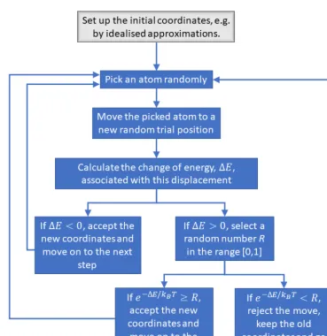
1. If the random number is between 0 and 𝑝𝑝, the move is accepted; if the random number is greater than 𝑝𝑝, the move is rejected [20]. This strategy ensures that a Boltzmann distribution of molecular configurations is produced in accordance with Eq. (13). Far more configurations are produced around the valleys of the energy surface and only a few are produced around the peaks, which means a considerable amount of computational effort is saved that would otherwise be wasted in probing the higher energy configurations that are physically less plausible.
Fig. 3: Metropolis sampling algorithm for the structural studies of molecular systems.
Once the physically plausible configurations are produced, the average of a property 𝐵𝐵 that is dependent on the atomic positions can be calculated using the simple relation
⟨𝐵𝐵⟩ =𝑀𝑀 k 1
W
&X!
𝐵𝐵(𝐪𝐪&),
(16)
where 𝑀𝑀 is the number of accepted configurations.
class of MC simulations, known as kinetic Monte Carlo (kMC), which does allow an explicit time coordinate. This is made possible by introducing rates of various events, which are inversely proportional to time. An event is essentially seen as a transition between one state to another and the rate of this is connected to the energy barrier that exists between the two states. We shall not discuss kMC in detail here since time dependence is not required in the structural studies of macromolecules.
4 Practical considerations
In this section we enlist a few practical points to be considered during a typical workflow of molecular simulation.
4.1 Connectivity in molecules
Specifying only the atomic coordinates, for instance through a PDB file, is not sufficient to carry out a molecular simulation. One also needs to provide information about the connectivity of atoms within a molecule. Many simulation packages have their own ways of defining the different types of chemical bonds that exist between the atoms. For biomolecules, one ‘standard’ way of doing this is through a PSF file (Protein Structure File). Despite what the name may suggest, PSF files are used to define connectivity within non-protein biomolecules as well. Automated ways of creating a PSF file from a given PDB file include the online tool CHARMM-GUI [21] and the AutoPSF plugin included in the VMD package [22]. CHARMM-GUI also has a tool to check for problems in a given PDB file and to some degree fix the file such that it is compatible with the CHARMM force field. It also has a tool to detect glycans and perform any necessary modifications in the PDB file arising from this. In case one of the automatic methods fails for some reason, a semi-automatic tool to create the PSF file is the psfgen tool that comes with VMD. It is semi-automatic in that a set of topology files and an input file specifying the type of bonds that are present among the various atomic species need to be provided by the user. While this may require careful treatment, it does give the user more precise control. The AutoPSF plugin in VMD, in fact, implements psfgen under the hood. VMD is also a powerful tool to visualise and manipulate PDB files and trajectory files that are output by many simulation packages.
4.2 Speed-up through coarse graining
Biomolecules can be very large for a molecular simulation. A typical protein may contain tens of thousands of atoms, while a DNA molecule may contain several billions of atoms. Obtaining explicit variation among all these atoms is not only computationally expensive, but also unnecessary in a large number of cases. To speed up the simulation, one may perform selective coarse graining by defining large regions of the molecule as ‘rigid’ and only small parts of the molecule as ‘flexible’. The rules of structural variation, according to either MD or MC, are then applied explicitly to all the atoms in the flexible regions and only to a representative point in each rigid region, which is usually the mid-point. The rigid regions can be identified by looking at the initial structure of the molecule. For instance, in a protein molecule one would find 𝛽𝛽-sheets that are made of several 𝛽𝛽-strands connected together and where motion beyond thermal vibrations does not occur. Assuming that the 𝛽𝛽-sheets are stable under normal physiological conditions, one could define these as rigid. Visibly thin regions of the molecule, such as linkers between domains, can be defined as flexible in order to drive structural variation. However, care must be taken so as to ensure that important bonds
such as disulphide bridges do not appear within a flexible region in a Monte Carlo simulation, as sudden variation from one state to another may break these bonds.
5 Inference of solution structure from scattering data
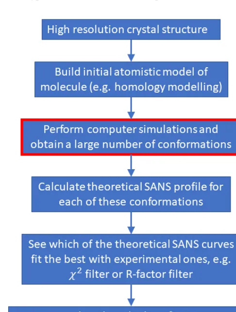
Once an ensemble of structures has been created by a simulation, calculating small angle neutron scattering (SANS) profiles is conceptually straightforward, although it may require some processing effort. Computationally one performs essentially the same procedure as in a real neutron scattering experiment, but this time in a virtual world, with a large set of PDB files of the molecular structures created by a simulation replacing the molecules that exist in a real experiment. A typical workflow of the whole process is shown in Figure 4.
Fig. 4: A typical workflow to infer atomistic structures of molecules in solution using SANS data.
5.1 Theoretical scattering profiles
𝐼𝐼(𝑄𝑄) = k k 𝑓𝑓&(𝑄𝑄)𝑓𝑓%(𝑄𝑄)sin (𝑄𝑄 ∙ 𝑟𝑟𝑄𝑄 ∙ 𝑟𝑟 &%) &% , W
%X! W
&X!
(17)
where 𝑄𝑄 is the scattering vector, 𝐼𝐼(𝑄𝑄) is the scattered intensity of the neutrons, 𝑟𝑟&% is the distance between atoms labelled 𝑖𝑖 and 𝑗𝑗 within the given theoretical conformation, 𝑓𝑓&(𝑄𝑄) is the form factor (or scattering factor) for atom 𝑖𝑖, which describes the scattering contribution of the stand-alone atom, and 𝑀𝑀 is the number of atoms in the molecule. Provided that the form factor is known for all the atomic species found in a biomolecule, only the interatomic distances, which are available from the generated PDB files, are required to calculate the scattering profiles from Eq. (17).
Implementation of Eq. (17) requires calculating 𝑀𝑀" terms for each conformation, which
can be computationally demanding when the molecule is large (large 𝑀𝑀) and there are a large number of conformations to go through. Approximation techniques have been reported that aim to reduce the burden of these calculations. These include the multipole expansion (ME) technique of Svergun et al. [24] and the golden vector method of Watson and Curtis [25] that scales linearly with the number of atoms in the molecule.
One thing that must be taken care of while calculating the theoretical scattering profiles is that the 𝑄𝑄-values must match those that are present in the experimentally obtained scattering curves. This is so that 𝐼𝐼(𝑄𝑄) for both the theoretical and experimental curves can be compared at exactly the same set of 𝑄𝑄-values. If this is not possible to achieve, one can interpolate the experimental data points at the desired set of 𝑄𝑄-values using, for instance, a spline method. If there is a mismatch in the 𝑄𝑄-values, there are likely to be significant errors in the subsequent analysis of the results; hence, this is an important step.
5.2 Identification of best-fit structures
The quality of a computationally generated atomistic conformation of the molecule can be tested by performing a statistical hypothesis test, such as an 𝑅𝑅-factor test (or sometime a 𝜒𝜒"
test). The 𝑅𝑅-factor is defined as
𝑅𝑅-factor as percentage = ∑ x>𝐼𝐼& YZ[L(𝑄𝑄&)> − 𝜂𝜂|𝐼𝐼\]GT^(𝑄𝑄&)|x ∑ >𝐼𝐼& YZ[L(𝑄𝑄&)> × 100,
(18)
where 𝐼𝐼YZ[L(𝑄𝑄&) and 𝐼𝐼\]GT^(𝑄𝑄&) denote the experimentally obtained and theoretically
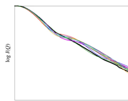
calculated scattering intensities, 𝜂𝜂 is a scaling factor used to match the theoretical curve to the experimental 𝐼𝐼(0) value and 𝑖𝑖 runs over the range of all the 𝑄𝑄-values over which the comparison of the curves is to be made. This method compares the scattering profile of each of the theoretical conformations and produces a numerical value of 𝑅𝑅-factor that indicates how closely the curve matches with the target experimental curve (Figure 5). The lower the 𝑅𝑅-factor, the better the fit.
Fig. 5: Comparison of the theoretically produced scattering profiles (non-black colours) with a single experimental profile (black).
Fig. 6: Identification of the best-fit structures using the 𝑅𝑅-factor filter. Each data point (circles) in this plot corresponds to a unique atomistic conformation produced by the molecular simulation. Yellow circles represent all the conformations that were created, while the best-fit 100 conformations with the lowest 𝑅𝑅-factors are shown in green.
A certain number of best-fit molecular structures identified in this way (e.g. the green points in Figure 6) can be subjected to further statistical or numerical analysis in order to reveal a common pattern within them. It must be stressed that a single structure is not sought to be identified here. Rather, a tightly-defined ensemble of structures is being obtained to match the solution structure of the biomolecules that are giving rise to the spherically averaged scattering curve in SANS experiments.
5.3 Web-based workflow
All the above steps outlined in this Chapter can be fairly demanding task for a non-expert. Preparing an input PDB file for simulation and then preparing the (complex) additional input files for performing the molecular simulations are not trivial tasks even for experts in the field. Not to mention the code to be written for the subsequent analysis of the results. An online free-to-use portal, SASSIE-web, simplifies this task considerably by presenting highly abridged web-based input forms for each of the tasks in the workflow [26]. It has modules to prepare structures, carry out simulations, calculate theoretical SAXS and SANS data and compare the outcome to experimental data. While the key outputs are shown on the web page after the calculations, one can download the more detailed files for further analysis.
6 Conclusions
Deducing the solution structure of biological macromolecules in solution is a complex task that requires expertise of several fields to be applied together. While SANS experiments are an effective way of capturing spherically averaged scattering profiles of the macromolecules, a computational counterpart of this process is required to exploit and decode the information provided by the experimental data. To this end, structural variation in a macromolecule can be performed using molecular simulations. Theoretical scattering profiles calculated from the
computationally generated structures can be compared with the experimental SANS curve to obtain a set of conformations that best reflect the structure of the macromolecule in solution.
References
1. L. Verlet, Phys. Rev. 159, 98 (1967).
2. M. P. Allen, D. J. Tildesley, Computer Simulation of Liquids (Clarendon Press, Oxford, 1989).
3. S. J. Weiner, P. A. Kollman, D. T. Nguyen, D. A. Case, J. Comp. Chem. 7, 230 (1986).
4. D. R. Langley, J. Biomol. Struct. Dyn. 16, 487 (1998).
5. K. Vanommeslaeghe, E. Hatcher, C. Acharya, S. Kundu, S. Zhong, J. Shim, E. Darian, O. Guvench, P. Lopes, I. Vorobyov, A. D. MacKerell jr., J. Comput. Chem. 31, 671 (2010).
6. G. Nemethy, M. S. Pottle, H. Scheraga, J. Phys. Chem. 87, 1883 (1983). 7. W. F. van Gunsteren and H. J. C. Berendsen, Groningen Molecular Simulation
(GROMOS) Library Manual (BIOMOS, Nijenborgh, 9747 Ag Groningen, 1987). 8. C. Oostenbrink, A. Villa, A. E. Mark, W. J. van Gunsteren, Comput. Chem. 25,
1656 (2004).
9. T. A. Soares et al., J. Comput. Chem. 26, 725 (2005).
10. N. L. Allinger, Y. H. Yuh, J.-H. Lii, J. Am. Chem. Soc. 111, 8551 (1998). 11. W. L. Jorgensen, J. D. Madura, C. J. Swenson, J. Amer. Chem. Soc. 106, 6638
(1984).
12. G. A. Kaminski et al., J. Comput. Chem. 23, 1515 (2002).
13. I. T. Todorov, W. Smith, K. Trachenko, M. T. Dove, J. Mater. Chem. 16, 1911 (2006).
14. J. C. Phillips, R. Braun, W. Wang, J. Gumbart, E. Tajkhorshid, E. Villa, C. Chipot, R. D. Skeel, L. Kale, K. Schulten. J. Comput. Chem. 26, 1802 (2005).
15. M. J. Abraham, T. Murtola, R. Schulz, S. Páll, J. C. Smith, B. Hess, E. Lindahl, SoftwareX 1-2, 19 (2015).
16. B. R. Brooks et al., J. Comput. Chem. 30, 1545 (2009). 17. S. Plimpton, J. Comp. Phys. 117, 1 (1995).
18. N. Metropolis, A. W. Rosenbluth, M. N. Rosenbluth, A.H. Teller, E. Teller, J. Chem. Phys. 21, 1087 (1953).
19. W. K. Hastings, Biometrika 57, 97 (1970).
20. C. J. Cramer, Essentials of Computational Chemistry (John Wiley & Sons, 2nd edn., 2004).
21. S. Jo, T. Kim, V. G. Iyer, and W. Im, J. Comput. Chem. 29, 1859 (2008). 22. W. Humphrey, A. Dalke, K., J. Schulten, Molec. Graphics 14, 33 (1996). 23. P. Debye, Ann. Phys. (Leipzig), 46, 809 (1915).
24. D. Svergun, C. Barberato, M. H. J. Koch, J. Appl. Cryst. 28, 768 (1995). 25. M. C. Watson and J. E. Curtis, J. Appl. Cryst. 46, 1171 (2013).