Stability analyses of two-temperature radiative shocks: formulation,
eigenfunctions, luminosity response and boundary conditions
Curtis J. Saxton
1,2,3Pand Kinwah Wu
1,41School of Physics, University of Sydney, NSW 2006, Australia
2Research School of Astronomy & Astrophysics, Australian National University, ACT 0200, Australia 3
Department of Theoretical Physics, Faculty of Science, Australian National University, ACT 0200, Australia 4
Mullard Space Science Laboratory, University College London, Holmbury St Mary, Dorking, Surrey RH5 6NT
Accepted 2001 January 15. Received 2001 January 3; in original form 2000 April 17
A B S T R A C T
We present a general formulation for stability analyses of radiative shocks with multiple cooling processes, longitudinal and transverse perturbations, and unequal electron and ion temperatures. Using the accretion shocks of magnetic cataclysmic variables as an illustrative application, we investigate the shock instabilities by examining the eigenfunctions of the perturbed hydrodynamic variables. We also investigate the effects of varying the condition at the lower boundary of the post-shock flow from a zero-velocity fixed wall to several alternative types of boundaries involving the perturbed hydrodynamic variables, and the variations of the emission from the post-shock flow under different modes of oscillations. We found that the stability properties for flow with a stationary-wall lower boundary are not significantly affected by perturbing the lower boundary condition, and they are determined mainly by the energy-transport processes. Moreover, there is no obvious correlation between the amplitude or phase of the luminosity response and the stability properties of the system. Stability of the system can, however, be modified in the presence of transverse perturbation. The luminosity responses are also altered by transverse perturbation.
Key words:accretion, accretion discs – shock waves – binaries: close – white dwarfs.
1 I N T R O D U C T I O N
The time-dependent properties of radiative shocks have been investigated by many researchers in different settings, for example the interactions between supernova shocks and the interstellar medium, and accretion flow onto compact objects (e.g. Falle 1975, 1981; Langer, Chanmugam & Shaviv 1981, 1982; Chevalier & Imamura 1982; Imamura, Wolff & Durisen 1984; Chanmugam, Langer & Shaviv 1985; Imamura 1985; Bertschinger 1986; Innes, Giddings & Falle 1987a,b; Gaetz, Edgar & Chevalier 1988; Wolff, Gardner & Wood 1989; Imamura & Wolff 1990; Houck & Chevalier 1992; Wu, Chanmugam & Shaviv 1992; To´th & Draine 1993; Dgani & Soker 1994; Strickland & Blodin 1995; Imamura et al. 1996; Wu et al. 1996; Saxton, Wu & Pongracic 1997; Hujeirat & Papaloizou 1998; Saxton et al. 1998; Saxton & Wu 1999). Many of these shocks are found to be thermally unstable. For instance, a numerical study by Langer et al. (1981) showed that the post-shock accretion flow in magnetic cataclysmic variables (mCVs), binaries in which a magnetic white dwarf accretes material from a red dwarf companion star, suffers thermal instabilities and hence fails to attain a steady state. The accretion shock is driven to oscillate, giving rise to quasi-periodic oscillations in the optical luminosity. A similar conclusion was obtained by Chevalier & Imamura (1982), using a linear perturbative analysis.
The stability of the radiative shock depends on the energy transport processes. In the case of accretion shocks in mCVs, thermal bremsstrahlung and cyclotron radiation are the most important cooling processes (e.g. King & Lasota 1979; Lamb & Masters 1979). Bremsstrahlung and cyclotron cooling have very different temperature dependences, and hence influence the stability properties of the accretion shock differently.
In the stability analysis of Chevalier & Imamura (1982), the total cooling effects were approximated by a single radiative loss term
L/ra
Tbdepending on temperatureTand densityr. Various choices of the power-law indices (e.g.a¼ 0:5 andb¼ 2 for bremsstrahlung
cooling) were investigated, and they have found that radiative shocks with largerb(i.e. stronger temperature dependence) are more stable against perturbations.
The individual cooling processes were subsequently considered explicitly in the numerical study of accretion onto magnetic white dwarfs by Chanmugam et al. (1985). An effective cooling term was constructed to mimic the effects caused by optically thick cyclotron cooling. Their study showed that efficient cyclotron cooling stabilizes the shock. Wu et al. (1992, 1996) further investigated the same system and found that in spite of the suppression of shock oscillations in the presence of cyclotron cooling, the oscillation frequency appears to increase quadratically with the magnetic field strength. Moreover, each of the cooling processes, bremsstrahlung and cyclotron, dominates in about half of the phases of an oscillatory cycle, allowing the perpetuation of small-amplitude oscillations provided that the magnetic field is moderate or weakðB&10 MGÞ.
Linear perturbative analyses of accretion shocks with bremsstrahlung and cyclotron cooling were carried out by Saxton et al. (1997). A composite cooling function (following Wu, Chanmugam & Shaviv 1994) was considered, comprising the sum of a term for bremsstrahlung cooling and an effective term for cyclotron cooling. The analysis was further extended by Saxton et al. (1998), in which the cooling function is a sum of terms for bremsstrahlung coolingðLbr/r2T0:5Þand a second power-law process with a destabilizing influenceðL2/r
aTbfor
b>1Þ. The cases considered included that of a cooling termðLcy/r0:15T2:5Þ, which effectively approximates the energy loss as a result of
cyclotron radiation in the geometry and flow conditions of the post-shock regions of mCVs. It was found that a simple comparison of cooling and oscillation time-scales is insufficient to understand the instabilities of the shock under various modes.
When the radiative cooling is fast compared to the electron – ion energy exchange, the electron and ion temperatures are generally unequal. Imamura et al. (1996) considered bremsstrahlung and Compton cooling, and a more general perturbation of the shock in both longitudinal and transverse directions. Their study showed that the electron – ion exchange process and the presence of transverse perturbations can destabilize each mode compared to the purely longitudinal and one-temperature cases. Saxton & Wu (1999) generalized the works of Chevalier & Imamura (1982), Imamura et al. (1996) and Saxton et al. (1997, 1998) for radiative accretion shocks by considering multiple cooling processes explicitly, the two-temperature effects and transverse perturbations (as for a corrugated shock). In the case of mCVs the introduction of two-temperature effects complicated and broke down the strictly monotonic stabilisation of modes with increasing cyclotron efficiency in one-temperature shocks with bremsstrahlung and cyclotron cooling, and the influence of transverse perturbation was not always able to destabilize oscillatory modes in the presence of both bremsstrahlung and cyclotron cooling. (For a review of stability of accretion shocks, see Wu 2000.)
The present paper expands upon the studies of the eigenvalue in Saxton & Wu (1999) to examine the amplitudes and phases of the eigenfunctions that describe the response of the post-shock structure to perturbations of the shock position. As an illustrative case we consider the accretion shocks of magnetic white dwarfs. Knowing the response of the hydrodynamic-variable profiles in turn provides information about other characteristics of thermally unstable shocks, such as the responses of post-shock emissions caused by the shock oscillations.
2 F O R M U L AT I O N
2.1 Hydrodynamics
In accretion onto white dwarfs, the supersonic flow meets a stand-off shock where the inwardly falling matter is abruptly decelerated to attain a subsonic speed. The shock sits above the white dwarf surface at a height xs<1=4vfftcool, where the free-fall velocity is
vff ¼ ð2GMwd/ RwdÞ1=2, the cooling time-scale istcool , nekBTs/L, andLis a radiative cooling function. (MwdandRwdare the white dwarf mass and radius respectively;kBis the Boltzman constant;neis the electron number density andTsis the shock temperature.)
The time-dependent mass continuity, momentum and energy equations for the post-shock accretion flow are
› ›t1v:7
r1rð7:vÞ ¼ 0; ð1Þ
r ›
›t1v:7
v17P ¼ 0; ð2Þ
› ›t1v:7
P 2gP r
› ›t1v:7
r ¼ 2ðg2 1ÞL; ð3Þ
› ›t1v:7
Pe 2g
Pe
r › ›t1v:7
r ¼ ðg 21ÞðG2 LÞ; ð4Þ
where the total radiative cooling functionLand the electron – ion energy exchange termGare local functions of the densityr, total pressureP, electron partial pressurePe, and the flow velocityv. The explicit form of the exchange function is
G ¼ 4
ffiffiffiffiffiffi
2p
p e4n
enilnC
mec
ui 2ðme/ miÞue
ðue1uiÞ3=2
whereni,eare the ion and electron number density, andui;e ¼kBTi;e/ mi;ec2withTi,ebeing the corresponding temperatures. The constants mi,eare the ion and electron masses,eis the electron charge,cis the speed of light and lnCis the Coulomb logarithm (as in e.g. Melrose 1986). An adiabatic indexg ¼5=3 for an ideal gas is assumed, and the equation of stateP ¼ rkBT/mmHis considered, wheremHis the mass of the hydrogen atom.
The total cooling function is written in a form of the bremsstrahlung-cooling term and a multiplicative term that expresses the ratio of the losses caused by the second cooling process and bremsstrahlung cooling. The second process is characterized by its power-law indices of density and electron pressureða ¼b21=2 andb ¼ 3=22a1bfor a general cooling termL2/raTbÞ, and by the parameteres, which is the relative efficiency evaluated at the shock. (Largeresimplies a more efficient second process.)
L;Lbr1L2 ¼Lbr½11esfðt0;peÞ; ð6Þ
and a function is defined to relate the primary and secondary cooling processes:
fðt0;peÞ;
4a1b
3a
11ss
ss
a
paetb0 ¼ Pe Pe;s
a
r rs
2b
; ð7Þ
wherePe,sandrsare the shock values of electron pressure and density. The dimensionless parameterss;ðPe/ PiÞsis the ratio of electron and
ion pressures at the shock. The bremsstrahlung cooling term Lbr ¼ Cr2ðPe/rÞ1=2, where the constant is
C ¼ ð2pkB/3meÞ
1=2ð
25pe6/3 hm
ec3Þðm/ kBm
3 pÞ
1=2
gB, with mpthe proton mass,hthe Planck constant,mthe mean molecular weight and gB <1 the Gaunt factor (see Rybicki & Lightman 1979). For completely ionized hydrogen plasma,m ¼ 0:5 and the constant has a value C<3:91016in cgs units.
2.2 Perturbation
A first-order perturbation is considered for the shock positionxsand velocityvs:
vs ¼ vs1eiky1vt; ð8Þ
xs ¼ xs01xs1eiky1vt; ð9Þ
wherevis the frequency, andkis the transverse wavenumber of perturbation in they(transverse) direction. The shock is at rest in the stationary solution, vs0 ¼0, and the perturbed motion of the shock has vs1 ¼ xs1v. The dimensionless frequency and transverse
wavenumber are
k ¼ xs0k; ð10Þ
d¼ xs0 vff
v: ð11Þ
The eigenfrequencies are complex,d¼ dR1idI, withdIbeing the dimensionless frequencies of the oscillations, anddRthe stability term. WhendRis positive the perturbation grows; whendRis negative the perturbation is damped.
The post-shock position coordinate is labelled byj;x/ xs, which isj ¼1 at the shock andj ¼0 at the white dwarf surface. The size of
the perturbation is parametrized by1;vs1/ vff ¼ dxs1/ xs0. The other scales to be eliminated arexs0(the stationary-state shock height) andra (the mass density of the pre-shock accretion flow). The hydrodynamic variables are expressed as
rðj;y;tÞ ¼ raz0ðjÞ½111lzðjÞeiky1vt; ð12Þ
vðj;y;tÞ ¼ 2 vfft0ðjÞ½111ltðjÞeiky1vt;1lyðjÞeiky1vt}; ð13Þ
Pðj;y;tÞ ¼ raðvffÞ2p0ðjÞ½111lpðjÞeiky1vt ð14Þ
and
Peðj;y;tÞ ¼ raðvffÞ2peðjÞ½111leðjÞeiky1vt: ð15Þ
wherez0,t0,p0andpeare dimensionless density, velocity, total pressure and electron pressure in the stationary solution; andlz,lt,ly,lp
andleare complex functions representing the response of the downstream structure to the perturbation of the shock height. These five functions describe perturbations of the density, longitudinal velocity, transverse velocity the total pressure and the electron pressure respectively.
Separating the time-independent terms from the hydrodynamic equations yields two algebraic equations and two differential equations for the stationary case:
p0 ¼12t0; ð17Þ
dj
dt0
¼ gp02 t0 ~
L ð18Þ
and
dpe
dt0
¼ 1 t0 12 ~ G ~ L
ðgp0 2t0Þ 2gpe
: ð19Þ
The electron – ion energy exchange and cooling processes are described by appropriate dimensionless forms:
~
G ¼ ðg 2 1Þ½raðvffÞ3/ xs021G ¼ ðg 21Þcccei
12t0 2 2pe
ffiffiffiffiffiffiffiffiffiffi t5
0p3e
q ; ð20Þ
~
L ¼ ðg 21Þ½raðvffÞ3/ xs021L¼ ðg 21Þcc
ffiffiffiffiffi pe
t3 0
r
½11esfðt0;peÞ; ð21Þ
where the constantccis determined by normalisation of the integrated stationary solution and the parameterceiis a ratio between the electron – ion energy exchange and radiative cooling time-scales, as described in Imamura et al. (1996) and Saxton & Wu (1999). The physical values ofccandceiare given in Saxton & Wu (1999) and Saxton (1999).
The first-order perturbation is determined by the matrix differential equation:
d dt0
lz lt ly lp le 2 6 6 6 6 6 6 6 6 4 3 7 7 7 7 7 7 7 7 5 ¼ 1 ~ L
1 2 1 0 1/t0 0
2 gp0/t0 1 0 2 1/t0 0
0 0 2 ðgp02 t0Þ/t0 0 0
g 2g 0 1=p0 0
g 2g 0 g/t0 2ðgp0 2t0Þ/t0pe
2 6 6 6 6 6 6 6 6 4 3 7 7 7 7 7 7 7 7 5 F1 F2 F3 F4 F5 2 6 6 6 6 6 6 6 6 4 3 7 7 7 7 7 7 7 7 5
; ð22Þ
where theFfunctions, which are composed of terms that do not include derivatives of thelvariables, are given by
F1ðt0;pe;jÞ ¼ 2jðlnt0Þ0 2 dlz1ikt0ly; ð23Þ
F2ðt0;pe;jÞ ¼ 2ðd2 t00Þlt1jðlnt0Þ01t00lz 2t00ðlp 2ltÞ; ð24Þ
F3ðt0;pe;jÞ ¼ 2ðd2 t00Þly1ikð12t0Þlp1ikt00j/d; ð25Þ
F4ðt0;pe;jÞ ¼ 2p0dðlp 2 glzÞ2 L~
3
2g2ðt0;peÞlz1 1
2g1ðt0;peÞle 2lt 2lp1 1
d 2
j t0
; ð26Þ
F5ðt0;pe;jÞ ¼ 2pedðle 2glzÞ 2L~
3
2g2ðt0;peÞlz1 1
2g1ðt0;peÞle 2 lt 2 le1 1
d 2
j t0
1G~ 5
2lz 2 3 2le1
p0lp 22pele
p0 22pe
2lt 2le1
1
d 2
j t0
; ð27Þ
where the primed quantities are derivatives in terms ofj. The functionsg1(t0,pe) andg2(t0,pe) are defined as
g1ðt0;peÞ ¼ 11
2esafðt0;peÞ
11esfðt0;peÞ;
ð28Þ
g2ðt0;peÞ ¼ 12
2 3
esbfðt0;peÞ
11esfðt0;peÞ
: ð29Þ
The complex matrix differential equation (22) can be decomposed into 10 first-order real differential equations in terms of the functions of the stationary solutionj(t0) andpe(t0), and the real and imaginary parts of each of the perturbed variables. It can be shown that equation (22) is the general description and that the more restricted formulations in Chevalier & Imamura (1982), Saxton et al. (1997, 1998) can be recovered from it under specific assumptions (Appendix A).
2.3 Cooling functions
self-consistent description of cyclotron loss usually requires solving the equations for radiative transfer and the hydrodynamics simultaneously. The particular geometry and physical conditions of the magnetically channelled accretion flow in mCVs, however, permit a simplification (see e.g. Cropper et al. 1999). A functional fit involving the density and temperature dependences of the cut-off frequency yields an approximate cooling termLcy/r0:15T2e:5(see Langer et al. 1982; Wu et al. 1994).
In our analysis the effective cyclotron cooling term has power-law indicesða;bÞ ¼ ð2:0;3:85Þ, and the efficiency parameteres(Wu 1994) depends upon the temperature, density, magnetic field, and geometry of the emission region. In the limit of a one-temperature accretion flow the efficiency of electron – ion energy exchangeceiis large, and the ratio of pressuressstends to unity. For two-temperature shocks,ssis determined by the electrons carrying energy into the region above the ion shock, which is a complication beyond the scope of this paper. Following Imamura et al. (1996) and Saxton & Wu (1999), we treatssas a parameter.
2.4 Stationary structure
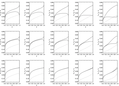
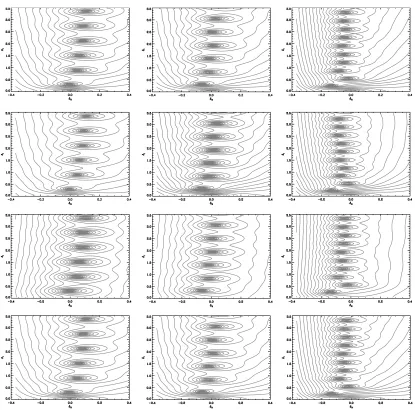
We assume the stationary wall condition, which requires a zero terminal velocity at the lower boundary. The stationary solution can be obtained by direct integration, after substituting equations (16) and (17) into equations (18) and (19). In Fig. 1 we show the stationary velocity structures (t0) of the post-shock region for various choices of the system parameters. The electron and ion sound speeds (ce,ci) are also plotted on the same scale. The density is related to the velocity byr0 ¼ ra/t0and the respective temperatures are proportional to the squared
sound speeds. Two-temperature effects are more significant in cases when cyclotron cooling is efficient (e.g.es ¼ 100Þ, and when the
electron – ion exchange is inefficient (i.e. smallcei). When two-temperature effects are unimportant, we recover the velocity, density and temperature structure of the one-temperature calculations (Wu 1994; Chevalier & Imamura 1982). A detailed discussion on the two-temperature stationary structures of the post-shock flows and their emission will be presented elsewhere (Saxton, Wu & Cropper, in preparation).
Figure 1.Stationary structures of the post-shock flow, witht0the flow velocity normalized tovff(dashed lines) as functions of the normalized positionj. The electron and ion sound speeds are represented by the upper and lower solid curves respectively. The upper, middle and lower rows represent parameter choices
2.5 Time-dependent solutions
For the time-dependent solution, the set of differential equations for the perturbed variables are integrated numerically from the shock down to the lower boundary for trial values of the complex eigenfrequencyd. The variables at the shock are determined by the shock-jump conditions:lz ¼ 0,lt ¼ 23,ly ¼ 3ik/d, andlp ¼le ¼ 2. The condition at the lower boundary is not so well-defined. The
stationary-wall condition only requires a zero terminal velocity at the bottom for the stationary solution. A lower boundary condition for the perturbed variables, such as the requirement that the flow should stagnateðlt ¼0Þ, the total pressure be constantðlp ¼0Þ, or some other condition
relating density, pressure and longitudinal velocity (e.g.lz1lt ¼ 0Þ, may be chosen.
The time-dependent solution can be expressed as a linear combination of oscillations of different eigenmodes. For a hydrodynamic variableX, we have
Xðj;tÞ ¼ X0ðjÞ
X
n
anlx;nðjÞexp vff
xs0
dnt
; ð30Þ
whereX0(j) is the stationary solution,anis the relative strength of the moden,dnis the eigenfrequency andlx,nis the eigenfunction. While
the complex d-eigenvalues provide information about the global stability properties and oscillating frequencies of the modes, the
l-eigenfunctions describe the more local dynamical properties. The absolute value of thel-function determines the local oscillation amplitude of the mode, and the phase indicates whether the oscillation of the hydrodynamic variables lags or leads in one region with respect to another.
3 E I G E N VA L U E S
The eigenvalues for two-temperature oscillating shocks with a ‘perfect’ stationary wall lower boundary condition, i.e.t ¼lt ¼0 (see
Saxton 2001), have been discussed in our previous paper (Saxton & Wu 1999, see also Imamura et al. 1996). More restricted studies on the one-temperature radiative shocks were presented in Saxton et al. (1997) and Saxton & Wu (1998) (see also Chevalier & Imamura 1982). Particular results of these studies include
(i) In the one-temperature case, the frequencies are quantized like modes of a pipe that is open at one end,dI<dIOðn21=2Þ1dCwith a
small correctiondC. When two-temperature effects are strong the, ‘stationary-wall’ condition at the lower boundary loses importance, and the frequency quantization becomes more like that of a doubly-open pipe, i.e.dI<dIOn.
(ii) The frequency spacingdIOdecreases as the efficiency of cyclotron cooling (es) increases, but tends to increase when the efficiency of electron – ion energy exchange (cei) decreases.
(iii) Increasingesgenerally stabilizes the modes, but when two-temperature effects are extreme there are situations in which an increase of
esdestablizes some modes.
(iv) In presence of transverse perturbation, there are maxima of instability at certain values of transverse wavenumber k for each longitudinal mode. However, there are values of (ss,cei,es,a,b) for which some longitudinal modes are stable at allkranges.
(v) For a given longitudinal mode, the shocks are generally stable against transverse perturbation of sufficiently largek.
(vi) Two-temperature effects affect the stability of cyclotron-cooling dominated shocks ðes@1Þ, but have less influence when
bremsstrahlung cooling dominatesðes<0Þ.
4 E I G E N F U N C T I O N S
4.1 Amplitude-profile
In one-temperature accretion shocks, the non-trivial eigenfunctions arelt,lp, andlz, corresponding to total pressure, longitudinal velocity
and density. In the two-temperature shocks, the non-trivial eigenfunctions also include that of the electron pressurele. When there is a transverse perturbation, a transverse perturbed velocity eigenfunctionlybecomes important also (see Section 7).
Our choice of boundary conditions requires that the perturbed longitudinal velocitylthas a fixed value of23 at the shock, and a
stagnant flow at the white dwarf surface implies a zeroltatj ¼0. (Here and hereafter in this section, unless specified, the stagnant flow
condition is assumed.) The amplitude profiles generally have local minima and maxima (see Appendix B), which are analogous to the nodes and antinodes in the oscillations of a pipe. The number of nodes and antinodes depends on the harmonic numbern, and their positions are determined by the radiative-transport processes and the system geometry. Unlike the nodes of an ideal pipe, the amplitude minima of oscillating shocks do not always go to zero, and the amplitude maxima do not have the same values. Moreover, the nodal features of one hydrodynamic variable may not coincide with those of another hydrodynamic variable.
4.1.1 |lt|-profile
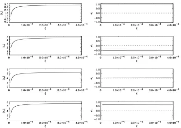
lower boundary, reaches a plateau or a peak at largerjand then declines with a gradual tail towards the shock boundary value. The rapid rise of |lt| occurs only in a small region wherej&1024, and the size of the region seems to be independent of the harmonic numbern(see
Fig. 2). The profiles fores ¼ 0 and 1 are similar, with the plateau value of |lt| of the fundamental mode<3 (e.g. Fig. B5). For higher
harmonics, the plateau values of |lt| are larger. The maxima (antinodes) generally become more visible whennincreases (e.g. Figs B6 – B8).
For the cases with largees, |lt| has a strong peak near the lower boundary. The peak heights tends to increase withn. It is worth noting
that in the extreme of smallcei, largessand largees(strong two-temperature effects and equal temperature for electrons and ions at the shock), a small peak in |lt| is also present near the shock (see appendix D.2.4 in Saxton 1999).
4.1.2 |lp|-profile
The boundary value of |lp| ¼ 2 at the shock, but it is not defined at the white dwarf surface for the stagnant flow condition. The |lp| profiles
do not show distinctive nodes and antinodes forn¼ 1 and 2. The nodes and antinodes, however, become more visible whennincreases and
ceibecomes small (see Figs B7 – B10).
4.1.3 |le|-profile
The electron pressure eigenfunctionsleshow nodes and antinodes. The sharpness of the nodes depends on the strength of the electron – ion energy exchange,cei. When the electron – ion energy exchange is efficient, the nodes are weak. When the electron – ion energy exchange is inefficient, (e.g.cei ¼ 0:1Þ, the amplitude minima are narrow injand deep in terms of amplitude. (See for example thees ¼100 curves of
Figs B1 – B4).
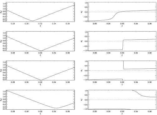
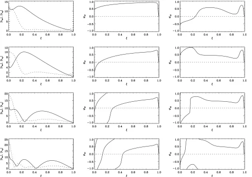
For two-temperature shocks, it is the electron pressureperather than the total pressurep0 that appears in the cooling terms and electron – ion exchange term. The electron pressure eigenfunction le therefore adopts the role that is played by the total pressure Figure 2.The amplified view |lt| profiles (left column) and the phaseswt(right column) near the lower boundary for the case withðss;cei;esÞ ¼ ð0:5;0:5;1:0Þ and a stagnant-flow boundary conditionðlt ¼0 atj ¼0Þ. The |lt| profiles and the phases of the modesn¼ 1, 2, 3 and 4 are shown in rows from top to
eigenfunctionlpin the one-temperature case. When the electron – ion energy exchange is weak (i.e. smallcei), thelpandleeigenfunctions are very different. The different modes have sharp and strikingly different features in |le|, whereas the total pressure eigenfunction is relatively featureless and smoothly varying. When the energy exchange between electrons and ions is efficient (i.e. largecei), the disparties between their pressures becomes small throughout most of the post-shock region. When the system approaches the one-temperature condition, and the total pressure follows the behaviour of the electron pressure, and the variations of the electron pressure and total pressure eigenfunctions,leandlp, are comparable in amplitude over allj.
Because of the lower boundary conditions we assume, the electron and ion temperatures are zero and the electron and ion pressures always become equal atj ¼0. The relative oscillation of the electron pressure must equal the relative oscillation of the total pressure at the lower boundary; i.e.leðjÞ !lpðjÞasj!0. However, there is no condition to determine the particular value at which these quantities must
meet atj ¼ 0, for any given mode under particular conditions.
4.1.4 |lz|-profile
The density eigenfunctions,lz, have strong and distinct nodes and antinodes. For each mode the positions and magnitudes of the node –
antinode – node sections are affected by the efficiency of cyclotron coolinges. Whenesis small (&1), the nodes are nearly evenly spaced and the antinodes near the shock tend to have lower amplitudes than those nearer the white dwarf surface. Whenesis larger, the nodes near the shock are more widely spaced and the antinodes near the shock tend to be higher in amplitude. The innermost antinode in the regionj&0:1 becomes higher asesincreases through the cases ofes ¼0, 1, 100 studied here.
Because of the sharp node and antinode features appearing in the profiles of |lz| (and |le|) we suspect that the density and electron pressure may be the quantities which determine the oscillatory properties of the shock. These hydrodynamic variables appear explicitly in the functions for the cooling and electron – ion energy exchange processes. Other hydrodynamic variables (i.e. the flow velocities and the total pressure) have amplitudes that vary less rapidly inj, probably indicating a less active involvement in determining the oscillatory behaviour of the shock.
For the studied cases of (ss,cei,es), the modes divide into two classes based on the qualitative features of their amplitude profiles. Profiles of the fundamental and first overtoneðn ¼1;2Þare more alike than the profiles of higher modes. Then. 2 modes haven22 nodes at intermediatejpositions, whereas then ¼1;2 profiles are slowly varying inj. The actual number of density nodes in each profile is
n21, including the shock (wherelz ¼ 0 is a boundary condition). An additional shallow, and usually indistinct, node occurs near the fixed
wall boundary (small j) for some cases of large es. When two-temperature effects are strong, |le| also has sharp nodes for n . 2 modes.
4.1.5 Nodes, antinodes and sound speeds
The dimensionless electron and ion sound speeds are given by
ce ¼ ffiffiffiffiffiffiffiffiffiffiffiffigt0pe
p
; ð31Þ
and
ci ¼
ffiffiffiffiffiffiffiffiffiffiffiffiffiffiffiffiffiffiffiffiffiffiffiffiffiffiffiffiffiffiffiffiffiffiffiffiffi gt0ð12 t0 2peÞ
p
ð32Þ
respectively, and the mean sound speed is
cs ¼
ffiffiffiffiffiffiffiffiffiffiffiffiffiffiffiffiffiffiffiffiffiffiffiffiffi gt0ð12 t0Þ
p
: ð33Þ
The sound speeds determine the local dynamical time- and length-scales, which influence the mode spacing. In regions of the post-shock flow where the sound propagation is fast, nodes of the eigenfunctions tend to be further apart.
The sound speeds generally decrease from the shock down to the lower boundary (see Fig. 1). When the gradients of the sound speed have change less dramatically (e.g. the casees ¼0 as in the far-left column of Fig. 1) the nodes of the eigenfunctions are more evenly
spaced. Whenesis large, the sound speeds are proportionately larger in the upper region of the flow, resulting in wider node-spacing in the high-jregion (contrast the differentescurves of |lz| in Fig. B4).
The local amplitudes of antinodes of the density eigenfunctions are greatest in regions near the shock for large es. This is counterintuitive, because previous studies (e.g. numerical simulations by Chanmugam et al. 1985, and Wu et al. 1992, 1996) show that oscillations aregloballysuppressed by cyclotron cooling. This global result would lead us to expect lower local amplitudes in the cyclotron-dominated region, and reduced amplitudes in systems with greateres. We believe that there is a connection between the increased antinode amplitudes and the increased node spacing in the cyclotron-dominated region whenesis great. The amplitude enhancement is not related to two-temperature effects, because it occurs in the one-temperature extreme (largeceiandss!1Þas well as the general two-temperature cases.
The behaviours of the nodes and antinodes (of the density eigenfunction) probably depend more sensitively on the overall form of the stationary solution than on the energy exchange processes present in each region of the flow.
4.2 Phase
The phases of the various perturbed hydrodynamic variables are given the labelswz,wt,wy,wpandwefor density, longitudinal velocity, transverse velocity, total pressure and electron pressure respectively. The zero values correspond to oscillations in phase with that of the shock height.
4.2.1 Boundary conditions and phase
At the shockðj ¼1Þthere are boundary conditions on all of thelvariables. The only phase which is not explicitly determined iswz. Our
There are fewer boundary conditions on the hydrodynamic variables at the bottom of the post-shock region. For the stationary-wall condition, only the longitudinal velocity variable is constrained; |lt|!0 asj!0. The phasewtis not determined. The other perturbed
variables have no definite lower boundary values, and their phases depend completely on the energy transport processes.
The phasesweandwpare not completely independent. As the electrons and ions have reached the same temperature at the lower
boundary, the oscillations of electron pressure and the oscillations of total pressure are identical atj ¼0. The variableslpandlehave the same values at the shock and the base but different values in between.
4.2.2 Interpretation ofdw/dj
If the phase increases withj, we consider the oscillation to be propagating downwards from the shock towards the lower boundary. (This is because the oscillations in the high-j region lead the oscillation in the lower-j regions.) If the phase decreases with j, then the oscillation is considered to be propagating upwards. The upward and downward propagation are labelled positive [1] and negative [2] respectively. If a complexl-function is viewed along thej-axis, with the real and imaginary l-parts horizontal and vertical, then the complex function appears to wind about the origin in either a clockwise manner for positive propagation, or an anticlockwise manner for negative propagation.
The phase functions can be regarded as having an overall winding betweenj ¼ 1 andj ¼0, with local phase glitches. For given (ss,
cei,es), the total winding of each perturbed variable across the interval 0 , j , 1 is a function of the harmonic numbern. The number of winding cycles is not necessarily an integer. Generally the number of cycles increases withn.
4.2.3 Illustrative cases
For the case of (ss, ceiÞ ¼ ð0:5;0:5Þ (see Figs B5 – B10), the pressure phaseswpand wewind positively for the first six modes when
es ¼0;1. Whenes ¼100,wemay wind negatively in some regions. Forn ¼1, the winding is negative throughout the entire post-shock region. Forn . 1 the winding is negative near the lower boundaryðj&0:05Þ, but it can be positive or negative elsewhere.
The phasewzwinds in a monotonically negative sense belowj&0:98 for the fundamental and first overtone. For the higher harmonics,
the winding ofwzundergoes one or more abrupt jumps or reversals in narrow ranges ofj. There aren22 phase jumps inwz, and their
positions correspond to the distinct density-amplitude nodes. For the harmonics withn . 2,wzbegins with a negative winding near the
shockðj ¼1Þand remains negatively winding throughout most of the flow, except at the jumps. The jumps can be either positive or negative. Descending from the shock, the first jump is positive, and for many choices of (ss,cei,es) andn, the second jump is negative. The signs of the further jumps depend on the mode and (ss,cei,es). For (ss,cei,esÞ ¼ ð0:5;0:5;1Þthe sequence of jumps is½ 1; 2 ; 2 whenn ¼ 5
ðes ¼ 0, 1 in Fig. B9) and½ 1; 2 ; 1 ; 2whenn ¼6ðes ¼0, 1 in Fig. B10). In cases where the cyclotron cooling dominates, the
positive jump inwzoccurs very close to the shock and the subsequent jumps are all negative and indistinct.
4.2.4 Phase ‘discontinuities’
The sense of a phase jump, e.g. either a modest negative jump in phase or a positive jump by more than half a cycle, is essentially distinct because the phase is seen to either increase or decrease asymptotically on either side of the node discontinuity, i.e. it is determined by the sign of 2dw/djin the neighbourhood. In some situations there are critical values ofesat which the sense of a phase jump changes from positive to negative. Foresfar from the critical values, phase jumps are gradual, being spread relatively broadly inj. At the criticalesthe phase jump is a discontinuity without a well-defined sign. Fig. 3 shows an example of the changes in structures of a density phase jump withesshown near and far from its transition value.
4.2.5 Phases atj ¼ 0
As not all the phases at the lower boundary are directly constrained by boundary conditions, they can only be obtained by integrating the hydrodynamic equations.
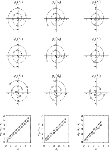
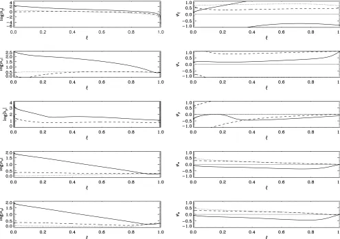
The lower boundary phase of each perturbed variable increases between a modenand the consecutive moden11, when (ss,cei,es) is fixed. This inter-mode increment differs slightly between the phases of different hydrodynamic variables. It also depends weakly on harmonic numbern. (See Fig. 4 for examples of lower boundary phases for one-temperature systems with different values of the parameteres.)
For a particular mode, there are regular phase relationships between different perturbed variables evaluated at the lower boundary. The general trends are as follows.
(i) For both one-temperature and two-temperature accretion flows, the density and longitudinal velocity profiles are approximately in phase (i.e.wz|j¼0<wt|j¼0Þ.
The phasingswa 2wbfor two hydrodynamic variablesaandbare approximately constant forn . 2. Forn ¼1 or 2 the phasings do not
conform to the general trend as well.
5 B O U N D A R Y C O N D I T I O N S
So far we have considered a special case of ‘stationary wall’ in which bothtandltare zero atj ¼0. We now consider modifications in
which the zero-velocity boundary condition for the stationary solutionðt0 ¼ 0 atj ¼ 0Þis retained but the boundary value ofltis not
necessarily zero. For example, the conditionlp ¼ 0 implies constant (non-oscillating) pressure at the lower boundary, whilst allowing
oscillations of the velocity at the base of the settling flow. Other interesting conditions studied includelz1lt ¼ 0 (opposite density and
velocity oscillations) andlz ¼ 0 (constant density at lower boundary), see Fig. 5. However, it is found that the change of boundary
conditions has little effect on the frequency sequencedI. The mode stabilitydRonly changes appreciably in the regime of largeesand high harmonic numbern. Some choices with reasonable physical interpretations In general most of the choices that we consider yield eigenvalues that are very close to those of the conventional caseðlt ¼0Þatj ¼ 0. Detailed discussions of the effects of boundary conditions on the
eigenfunctions can be found in Saxton (2001).
Alternative lower boundary conditions on the stationary variables may be considered in conjunction with alternative conditions on the perturbed variables. However these choices would describe systems that are physically very different from the white dwarf accretion problem illustrated in this paper. An exploration of the properties of such systems is beyond the scope of this paper, and will be investigated in the future.
6 L U M I N O S I T Y R E S P O N S E
The total power (normalized torav2ffÞ is given by integrating the cooling function over the whole post-shock structure in the stationary
solution:
L ¼
ð1
0
~
L
g2 1dj ¼
ð1=4
0
½gð12t0Þ2 t0
g2 1 dt0 ¼
7g 2 1
32ðg2 1Þ: ð34Þ
For the adiabatic indexg ¼5=3, the total power radiated via all processes isL ¼ 1=2, consistent with energy-conservation. The contribution of bremsstrahlung cooling is
Lbr;0 ¼
ð1=4
0
½gð12t0Þ 2t0
g 21
1 11 L~cy/L~br
dt0: ð35Þ
Figure 4.Phase of perturbed variables evaluated at the lower boundaryðj¼ 0Þfor then¼ 1;…;8 modes of one-temperature systems. Phases are defined in
The second cooling process (which is assumed to be cyclotron cooling) contributes the difference between this value and the total,
Lcy;0 ¼ L 2Lbr;0.
It can be shown that the local luminosity responses are described by complexl-functions that are analogous to the eigenfunctions of the hydrodynamic variables. The bremsstrahlung and cyclotron luminosity response functions, normalized to1, are
lbr ¼
3 2lz1
1
2le ð36Þ
and
lcy ¼ ð0:15 22:5Þlz12:5le ð37Þ
for the conditions of accreting magnetic white dwarfs. For a particular mode thelbrandlcyprofiles describe what could be regarded as eigenfunctions of the effect of the oscillations on the cooling emission.
the antinodes oflbroccur at the nodes oflcyand the nodes oflbroccur at the antinodes oflcy. There is no obvious relation between the luminosity responseslbr,lcyand the eigenvaluesd.
Multiplyinglbr andlcyby the respective cooling functions and integrating over the entire post-shock region yields the luminosity responses for a small shock-height perturbation1(see Section 2.2):
Lbr;1 ¼1
ð1=4
0
~
Lbr
g 21lbr dj
dt0
dt0 ¼ 1
ð1=4
0
½gð12 t0Þ 2t0
g 21
~
Lbr
~
Lbr1L~cy
lbrdt0; ð38Þ
and
Lcy;1 ¼1
ð1=4
0
~
Lcy
g 2 1lcy dj
dt0
dt0 ¼ 1
ð1=4
0
½gð12 t0Þ 2 t0
g 21
~
Lcy
~
Lbr1L~cy
lcydt0: ð39Þ
Lbr,1is different for different modes, and so isLcy,1. Moreover,the modes which have high-amplitudeLcy,1oscillations do not necessarily have strong oscillations inLbr,1.
In Table 1 we show the integrated luminosity responses, scaled according to the amplitude of the shock-height oscillation1. These quantities are proportional to the relative variations in bremsstrahlung (cyclotron) emission.
Lbr,1andLcy,1do not show obvious dependence ondR, however, they do seem to be dependent on the system parameters (ss,cei,es). Whether or not |Lbr;1|/ Lbr;0 . |Lcy;1|/ Lcy;0depends strongly ones, but is only weakly dependent onssandcei.
The complex phases of the valuesLbr,1and Lcy,1 areFbr(n) and Fcy(n) respectively for each mode n, and are listed in Table 2. Depending on the difference between the phases, the waxing and waning of the emission as a result of one cooling process may follow or lead the other process, or else they may be in phase or antiphase.
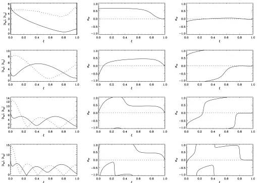
Figure 6. Profiles of luminosity perturbed variables, lbr and lcy, in modes n¼1, 2, 3, 4 from top to bottom. This choice of system parameters,
For smallesand for a given moden, the phasesFbr(n) andFcy(n) are nearly constant throughout the (ss,cei) parameter space. The two-temperature parameters (ss, cei) are almost ineffectual in the small-esregime. For constant ssand es, decreasing cei causes the phase differenceFcyðnÞ 2 FbrðnÞto decrease. This means that if cyclotron luminosity lags then its lag increases; if cyclotron luminosity leads
bremsstrahlung luminosity then the cyclotron lead decreases.
In general,Fbrð1Þ<0:35pto 0.5pandFcyð1Þ<0:9pfor the fundamental mode in a wide range of system parameters, i.e. cyclotron
emission oscillation almost always lags bremsstrahlung emission by<0:6p. In the extreme cases in which two-temperature effects are so strong that the fundamental mode becomes unstable, e.g. whenðss;cei;esÞ ¼ ð1:0;0:1;100Þ, this relation breaks down. The phase properties
are more complicated for the overtones because of the more complicated winding and nodes in thel-functions (see 4.2.2). Therefore no obvious relationships are found between the stability of a mode, the phasesFbr,Fcy, and their differences.
7 T R A N S V E R S E P E R T U R B AT I O N
7.1 Eigenfunction profiles
In the absence of transverse perturbationsðk ¼0Þ, the transverse velocity eigenfunctionlyis zero everywhere. Whenk . 0, the profiles of
the other eigenfunctions are modified (see Figs 8 and 9). The amplitude |ly| generally has its maximum value near the lower boundary, and
from that value it declines steeply injto the value fixed by the boundary condition at the shock. Increasingkcauses the amplitude |ly| to
increase in the region near the lower boundary, and the slope d|ly|=djsteepens throughout the profile. Greateresmakes the slope steeper, whenkis fixed. For somekthere are one or more local minima in the |ly| profile, with the number of minima depending on the harmonic
numbern.
The transverse velocity phasewygenerally winds in a negative sense from the shock to the lower boundary (see 4.2.2). The total number
of turns ofwyincreases withkuntil a threshold is reached. Beyond the threshold there is no winding inwy(see Figs 8 and 9, third panel, right
column). The lower boundary values of |lz|, |lt|, |lp| and |le| all increase withkbeyond thek-threshold.
The |lz| and |lt| profiles have the most distinctive features. However thelzandltfeatures disappear whenkis sufficiently large. These
Table 1. Amplitudes of the oscillations of the total emission in bremsstrahlung and cyclotron radiation, relative to these processes total luminosities in the stationary solution. For each set of the system parameters, the left column indicates whether the mode is stable (2) or unstable (1) in the small-amplitude analysis (see complete eigenvalue results in Saxton & Wu 1999). The middle and right columns are the1-normalized relative amplitudes |Lbr;1|/1Lbr;0and |Lcy;1|/1Lcy;0respectively.
ss cei es ¼0 es ¼ 1 es ¼ 100
dR |
Lbr;1| 1Lbr;0
|Lcy;1| 1Lcy;0 dR
|Lbr;1| 1Lbr;0
|Lcy;1| 1Lcy;0 dR
|Lbr;1| 1Lbr;0
|Lcy;1| 1Lcy;0
0.2 0.1 2 2.749 * 2 0.924 2.615 2 0.534 0.796
1 1.650 * 2 0.333 0.736 2 0.203 0.405
1 2.501 * 2 0.945 0.588 2 0.471 1.156
1 1.298 * 1 0.859 0.473 2 0.566 0.927
1 1.685 * 2 1.085 0.375 2 0.544 0.728
1 2.020 * 1 0.978 0.352 2 0.741 0.594
0.2 0.5 2 2.732 * 2 1.136 3.755 2 1.128 4.057
1 1.626 * 2 0.213 0.659 2 0.145 0.825
1 2.493 * 2 1.001 0.202 2 0.471 0.964
1 1.294 * 2 0.819 0.364 2 0.525 1.093
1 1.651 * 2 1.107 0.354 2 0.484 0.923
1 1.977 * 2 0.987 0.329 2 0.688 0.795
0.2 1.0 2 2.732 * 2 1.219 4.227 2 1.244 5.198
1 1.621 * 2 0.168 1.193 2 0.246 1.072
1 2.494 * 2 1.054 0.260 2 0.352 0.400
1 1.291 * 2 0.788 0.099 2 0.550 0.806
1 1.654 * 2 1.099 0.214 2 0.416 0.924
1 1.974 * 2 0.998 0.248 2 0.641 0.863
0.5 0.1 1 2.800 * 2 1.277 2.857 2 0.661 0.695
1 1.628 * 1 0.435 0.727 2 0.279 1.751
1 2.530 * 1 1.218 0.693 2 0.612 1.494
1 1.335 * 1 1.096 0.633 1 0.693 1.429
1 1.652 * 1 1.243 0.557 1 0.860 1.315
1 2.049 * 1 1.209 0.528 1 0.923 1.215
0.5 0.5 2 2.745 * 2 1.318 4.079 2 1.254 3.600
1 1.618 * 2 0.345 0.513 2 0.183 0.429
1 2.497 * 2 1.197 0.190 2 0.715 0.950
1 1.306 * 1 1.015 0.344 2 0.652 1.173
1 1.641 * 1 1.228 0.339 2 0.804 1.143
1 1.983 * 1 1.109 0.331 2 1.102 1.080
0.5 1.0 2 2.739 * 2 1.342 4.453 2 1.425 4.649
1 1.617 * 2 0.304 0.950 2 0.294 0.898
1 2.496 * 2 1.215 0.237 2 0.677 0.171
1 1.297 * 1 0.987 0.199 2 0.666 0.758
1 1.650 * 2 1.228 0.231 2 0.643 0.929
1 1.976 * 1 1.091 0.232 2 1.109 0.959
1.0 0.1 1 2.893 * 2 1.635 2.419 1 0.738 0.580
1 1.601 * 1 0.516 1.024 1 0.350 2.706
1 2.596 * 1 1.438 1.070 1 0.654 2.588
1 1.396 * 1 1.278 1.043 1 0.814 2.533
1 1.591 * 1 1.319 0.975 1 1.192 2.430
1 2.094 * 1 1.388 0.917 1 1.013 2.311
1.0 0.5 2 2.769 * 2 1.551 4.088 2 1.277 3.048
1 1.604 * 1 0.415 0.419 1 0.211 0.512
1 2.505 * 1 1.373 0.284 2 0.806 1.494
1 1.329 * 1 1.141 0.402 2 0.662 1.737
1 1.624 * 1 1.303 0.395 2 1.128 1.778
1 1.998 * 1 1.270 0.402 2 1.202 1.739
1.0 1.0 2 2.752 * 2 1.544 4.516 2 1.441 4.218
1 1.609 * 1 0.384 0.780 2 0.311 0.462
1 2.499 * 1 1.374 0.246 2 0.822 0.615
1 1.309 * 1 1.108 0.251 2 0.672 1.115
1 1.640 * 1 1.299 0.246 2 0.905 1.319
Table 2. Total bremsstrahlung and cyclotron emission phases,FbrandFcy, expressed as multiples ofp, for the modesn¼ 1…6 from top to bottom, under given (ss,cei,es) conditions. In this convention the phase of the shock-position oscillation is defined asFs ¼ 0. In each set, the third column described the difference between the phases of integrated cyclotron- and bremsstrahlung-luminosity oscillations, FcyðnÞ2FbrðnÞ. Negative values indicate the cyclotron luminosity oscillation following the bremsstrahlung luminosity oscillation; and positive values indicate cyclotron luminosity leading bremsstrahlung luminosity.
ss cei es ¼ 0 es ¼ 1 es ¼ 100
Fbr2Fs Fcy 2Fs Fcy2Fbr Fbr2Fs Fcy 2Fs Fcy2Fbr Fbr2Fs Fcy 2Fs Fcy2Fbr
0.2 0.1 20.366 * * 20.353 20.986 20.663 20.542 0.928 20.530
20.763 * * 0.573 20.336 20.909 0.388 20.385 20.773
20.450 * * 20.891 20.319 0.572 0.770 20.429 0.801
0.141 * * 20.333 20.263 0.070 20.855 20.295 0.560
0.936 * * 0.305 20.280 20.585 20.325 20.271 0.054
20.454 * * 0.892 20.302 20.194 0.144 20.281 20.425
0.2 0.5 20.374 * * 20.347 20.989 20.642 20.410 0.954 20.636
20.766 * * 0.517 20.989 0.494 20.163 20.645 20.482
20.458 * * 20.957 20.334 0.623 0.725 20.367 0.908
0.116 * * 20.441 20.207 0.234 0.955 20.373 0.672
0.913 * * 0.175 20.168 20.343 20.600 20.324 0.276
20.487 * * 0.674 20.170 20.844 20.137 20.265 20.128
0.2 1.0 20.376 * * 20.339 20.981 20.642 20.340 20.984 20.644
20.767 * * 0.396 0.993 0.597 20.284 20.827 20.543
20.461 * * 20.973 0.934 20.093 0.810 20.607 0.583
0.111 * * 20.487 20.107 0.380 0.879 20.335 0.786
0.909 * * 0.147 20.050 20.197 20.868 20.324 0.544
20.494 * * 0.612 20.071 20.683 20.244 20.299 20.055
0.5 0.1 20.361 * * 20.348 20.976 20.628 20.486 20.981 20.495
20.762 * * 0.635 20.157 20.792 0.402 20.231 20.633
20.448 * * 20.771 20.192 0.579 0.775 20.251 0.974
0.123 * * 20.863 20.284 0.579 20.738 20.192 0.546
0.931 * * 0.484 20.252 20.736 20.241 20.182 0.059
20.466 * * 20.863 20.284 0.579 0.219 20.195 20.414
0.5 0.5 20.373 * * 20.349 20.995 20.646 20.415 0.976 20.609
20.766 * * 0.615 0.825 0.210 20.047 20.585 20.538
20.458 * * 20.820 0.077 0.897 0.743 20.202 20.945
0.112 * * 20.240 20.024 0.216 20.923 0.270 0.807
0.911 * * 0.406 20.054 20.460 20.399 20.211 0.188
20.490 * * 20.974 20.105 0.869 20.021 20.189 20.168
0.5 1.0 20.375 * * 20.347 20.992 20.645 20.359 20.980 20.621
20.768 * * 0.593 0.884 0.291 20.160 20.878 20.718
20.461 * * 20.833 0.660 20.507 0.782 0.171 20.611
0.123 * * 20.260 0.235 0.495 0.986 20.187 0.827
0.907 * * 0.388 0.137 20.251 20.458 0.193 0.651
20.496 * * 0.996 0.047 20.949 20.083 20.187 20.104
1.0 0.1 20.352 * * 20.342 20.889 20.547 20.474 20.299 0.175
20.757 * * 0.700 20.134 20.834 0.418 20.104 20.522
20.444 * * 20.690 20.195 0.495 0.762 20.146 20.908
0.091 * * 20.109 20.243 20.134 20.639 0.497 20.864
0.924 * * 0.573 20.292 20.865 20.227 20.159 0.068
20.487 * * 20.772 20.325 0.447 0.251 20.181 20.432
1.0 0.5 20.371 * * 20.352 20.986 20.634 20.428 0.994 20.578
20.766 * * 0.684 0.689 0.005 0.039 20.067 20.106
20.458 * * 20.734 0.113 0.847 0.731 20.070 20.801
0.104 * * 20.141 0.008 0.149 20.814 20.121 0.693
0.906 * * 0.533 20.047 20.580 20.306 20.137 0.169
20.494 * * 20.817 20.111 0.706 0.039 20.149 20.188
1.0 1.0 20.374 * * 20.353 20.991 20.638 20.378 20.975 20.597
20.768 * * 0.680 0.807 0.127 20.088 20.950 20.862
20.461 * * 20.743 0.525 20.732 0.755 0.056 20.699
0.105 * * 20.151 0.241 0.392 20.928 20.063 0.865
0.904 * * 0.526 0.160 20.366 20.328 20.093 0.235
k-dependent properties depend on the harmonic number nand the system parameters [e.g.k*4 forðss;cei;esÞ ¼ ð0:5;0:5;100Þand
n¼ 1;2;k*8 forðss;cei;esÞ ¼ ð0:5;0:5;0Þandn ¼1;2.
The amplitude and phase profiles of the total pressurelpand electron pressureleare less dependent uponkthan the density and velocity eigenfunctions. In the case ofðss;ceiÞ ¼ ð0:5;0:5Þthe eigenfunctions for total pressure and electron pressure are not greatly affected by the
introduction of a transverse perturbation whenkis small. The total pressure and electron pressure eigenfunctions are much alike because the amplitude and phase profiles match at both the upper and lower boundaries. Increasingkcauses the decrease of the lower boundary pressure phase,we|j¼0 ¼ wp|j¼0. The phaseswpandwehave similar profiles for small-esflows, but the electron pressure develops phase jumps and associated node-like amplitude features whenesis large. (For a more detailed discussion of the transverse perturbation, see Saxton 1999.)
7.2 Luminosity response
Figs 10 and 11 show the luminosity responses as functions ofkforn ¼1 and 2. The integrated luminosity amplitudes |Lbr,1| and |Lcy,1| have minima inkwhere there are abrupt changes of the phasesFbrandFcyrespectively. The number ofk-minima is determined byn. Forn ¼1 and ðss;ceiÞ ¼ ð0:5;0:5Þ the |Lbr,1| minima occur at about k , 1:6, 1.0, 0.6 for es ¼ 0, 1, 100 and the |Lcy,1| minima coincide at approximately the samek-values. Forn¼ 2 there are at most two minima of |Lbr,1|. For smallesthe minimum corresponding to a larger
k-value becomes an inflection, e.g. fores ¼ 0 the actual amplitude minimum of |Lbr,1| is atk<1:8 and the inflection point is atk<3:4. Both amplitudes, |Lbr,1| and |Lcy,1|, are slowly varying inkwhen the value ofkis belowk*, wherek*ðn;esÞ<12ð2n21ÞkeðesÞandke
depends on the system parameters. Forðss;ceiÞ ¼ ð0:5;0:5Þ,ke , 1:0 fores ¼0. It reduces gradually as the cooling efficiency increases,
andke , 0:3 ates ¼ 100. For wavenumbersk . k*, both |Lbr,1| and |Lcy,1| increase rapidly withk. This is a consequence of the increasing amplitudes of the hydrodynamic variables’l-functions askincreases. Because bremsstrahlung cooling is most efficient in regions near the lower boundary, |Lbr,1| tends to rise more steeply withkthan |Lcy,1| does.
The integrated luminosity phasesFbrandFcywind withk. On top of these winding trends, there are phase jumps where the respective
|Lbr,1|, |Lcy,1| amplitudes reach minima. Away from the minima, both of the phases generally decrease whenk increases. Generally the winding of both phases inkis more rapid whenesis large, however for sufficiently largeesthere are modes whereFbrovertakesFcyin its variation withk, e.g.n ¼ 2 withðss;cei;esÞ ¼ ð0:5;0:5;100Þ. The prevailing winding of the bremsstrahlung phaseFbris usually more sensitive tokthan theFcyis, i.e. 2 dFbr/dktends to be greater than 2dFcy/dk.
In summary, the presence of transverse perturbations may significantly alter the instability of a mode and modify the luminosity response.
8 C O N C L U S I O N S
We have presented a general formulation for the linear analysis of two-temperature radiative shocks with multiple cooling processes. The formulation recovers the restrictive cases in the previous studies such as the one-temperature flows with a single cooling function (Chevalier & Imamura 1982), the one-temperature flows with multiple cooling processes (Saxton et al. 1998) and the two-temperature flows with a single cooling function (Imamura et al. 1996). We have applied the formulation to mCVs and investigated the hydrodynamic and emission properties of the time-dependent post-shock accretion flows in these systems. Our finding are summarized as follows.
The amplitude profiles ofl-eigenfunctions show local minima and maxima, which we identify as nodes and antinodes. The nodes and antinodes are prominent only in the eigenfunction profiles of density and electron-pressure. The eigenfunctions for the fundamental and first overtone are more similar to each other than any of the higher overtones. The eigenfunctions for higher-order modes have more nodes.
The phase profiles of the eigenfunctions describing particular hydrodynamic variables circulate about the complex plane asjvaries from the shock down to the lower boundary. This circulation can be positive or negative overall, or there may be reversals of the winding sense between distinct zones. The abrupt jumps in the phase profiles always coincide with the nodes in thel-eigenfunction profiles.
The luminosity responses of cyclotron and bremsstrahlung are determined by the l-eigenfunctions. There is no obvious general relationship between the amplitude or phase luminosity responses and the stability properties of the flow. There are situations in which a mode is unstable but the amplitude of oscillations are larger in the cyclotron luminosity than in the bremsstrahlung luminosity.
Figure 10.Integrated luminosity response amplitudes and phases forn ¼1 mode in the presence of transverse perturbations, for the parametersðss;ceiÞ ¼
ð0:5;0:5Þandes ¼0, 1, 100 from left to right. The curves corresponding to bremsstrahlung cooling are marked with1; the curves corresponding to cyclotron cooling are marked with.
For the same stationary condition ðt ¼ 0 atj ¼ 0Þ, all our choices of perturbed boundary conditions do not show significant differences in the stability properties. We therefore conclude that the stability properties of the flow with a stationary wall boundary is mainly determined by the energy-transport processes.
The presence of a transverse perturbation modifies the eigenfunction profiles of all the hydrodynamic variables. The profiles of electron-pressure and total-electron-pressure eigenfunctions are less affected in comparison with the other eigenfunction profiles. In some range of the transverse wavenumberk, the density and longitudinal velocity eigenfunction profiles develop extra node features. Whenkis large enough (&3 forn¼ 1;2Þ, the amplitudes of all the eigenfunctions become large near the lower boundary. The amplitudes, however, decrease as the heightjincreases. For some values of the transverse wavenumberð1&k&3Þ, a mode which is stable in the absence of the transverse perturbation can become unstable. However, whenkis very large, the mode is stabilized. The phase difference between the oscillations in the bremsstrahlung and cyclotron luminosity are also modified in the presence of transverse perturbations.
R E F E R E N C E S
Bertschinger E., 1986, ApJ, 304, 154
Chanmugam G., Langer S. H., Shaviv G., 1985, ApJ, 299, L87 Chevalier R. A., Imamura J. N., 1982, ApJ, 261, 543
Cropper M., Wu K., Ramsay G., Kocabiyik A., 1999, MNRAS, 306, 684 Dgani R., Soker N., 1994, ApJ, 434, 262
Gaetz T. J., Edgar R. J., Chevalier R. A., 1988, ApJ, 329, 927 Falle S. A. E. G., 1975, MNRAS, 172, 55
Falle S. A. E. G., 1981, MNRAS, 195, 1011 Houck J. C., Chevalier R. A., 1992, ApJ, 395, 592 Hujeirat A., Papaloizou J. C. B., 1998, A&A, 340, 593 Imamura J. N., 1985, ApJ, 296, 128
Imamura J. N., Wolff M. T., 1990, ApJ, 355, 216
Imamura J. N., Wolff M. T., Durisen R. H., 1984, ApJ, 276, 667
Imamura J. N., Aboasha A., Wolff M. T., Wood K. S., 1996, ApJ, 458, 327 Innes D. E., Giddings J. R., Falle S. A. E. G., 1987a, MNRAS, 224, 179 Innes D. E., Giddings J. R., Falle S. A. E. G., 1987b, MNRAS, 226, 67 King A. R., Lasota J. P., 1979, MNRAS, 188, 653
Lamb D. Q., Masters A. R., 1979, ApJ, 234, L117
Langer S. H., Chanmugam G., Shaviv G., 1981, ApJ, 245, L23 Langer S. H., Chanmugam G., Shaviv G., 1982, ApJ, 258, 289
Melrose D. B., 1986, Instabilities in Laboratory and Space Plasmas. Cambridge Univ. Press, Cambridge Rybicki G. B., Lightman A. P., 1979, Radiative Processes in Astrophysics. John Wiley & Sons, New York Saxton C. J., 1999, PhD Thesis, Univ. Sydney
Saxton C. J., 2001, Publ. Astron. Soc. Aust., submitted Saxton C. J., Wu K., 1999, MNRAS, 310, 677
Saxton C. J., Wu K., Pongracic H., 1997, Publ. Astron. Soc. Aust., 14, 164 Saxton C. J., Wu K., Pongracic H., Shaviv G., 1998, MNRAS, 299, 862 Strickland R., Blodin J. M., 1995, ApJ, 449, 727
To´th G., Draine B. T., 1993, ApJ, 413, 176
Wolff M. T., Gardner J., Wood K. S., 1989, ApJ, 346, 833 Wu K., 1994, Publ. Astron. Soc. Aust., 11, 61
Wu K., 2000, Space Sci. Rev., 93, 611
Wu K., Chanmugam G., Shaviv G., 1992, ApJ, 397, 232 Wu K., Chanmugam G., Shaviv G., 1994, ApJ, 426, 664
Wu K., Pongracic H., Chanmugam G., Shaviv G., 1996, Publ. Astron. Soc. Aust., 13, 93
A P P E N D I X A : R E D U C T I O N T O R E S T R I C T E D S Y S T E M S
The matrix equation describing the perturbation is
d dt0
lz lt ly lp le 2 6 6 6 6 6 6 6 6 4 3 7 7 7 7 7 7 7 7 5 ¼ 1 ~ L
1 2 1 0 1/t0 0
2 gp0/t0 1 0 2 1/t0 0
0 0 2 ðgp02 t0Þ/t0 0 0
g 2g 0 1=p0 0
g 2g 0 g/t0 2ðgp0 2t0Þ/t0pe
2 6 6 6 6 6 6 6 6 4 3 7 7 7 7 7 7 7 7 5 F1 F2 F3 F4 F5 2 6 6 6 6 6 6 6 6 4 3 7 7 7 7 7 7 7 7 5
: ðA1Þ
For systems with a purely longitudinal perturbation,k ¼ 0 and the third row and third column of the matrix can be eliminated. Thelyterms
ðlnlyÞ0 ¼d/t0 2ðlnt0Þ0, orl0y ¼lyðd2t00Þ/t0. The two-temperature system with purely longitudinal perturbations is described by this
reduced matrix equation, with correspondingFfunctions that omit all terms ofly:
d dt0
lz lt lp le 2 6 6 6 6 6 4 3 7 7 7 7 7 5 ¼ 1 ~ L
1 21 1/t0 0
2gp0/t0 1 21/t0 0
g 2 g 1=p0 0
g 2 g g/t0 2ðgp0 2t0Þ/t0pe
2 6 6 6 6 6 4 3 7 7 7 7 7 5 F1 F2 F4 F5 2 6 6 6 6 6 4 3 7 7 7 7 7 5
: ðA2Þ
In the single-temperature limit,ceibecomes large and the electron and ion pressures both equal half of the total pressure, i.e. we have 2pe!p0 ¼12 t0, andle!lpthroughout the entire post-shock flow. Moreover,F5!1=2F4. Then we can eliminate the fifth row of (A1),
yielding
d dt0
lz lt ly lp 2 6 6 6 6 6 4 3 7 7 7 7 7 5 ¼ 1 ~ L
1 21 0 1/t0
2gp0/t0 1 0 21/t0
0 0 2ðgp0 2t0Þ/t0 0
g 2 g 0 1=p0
2 6 6 6 6 6 4 3 7 7 7 7 7 5 F1 F2 F3 F4 2 6 6 6 6 6 4 3 7 7 7 7 7 5
: ðA3Þ
Reducing the system to a one-temperature form with purely longitudinal perturbations leaves only three non-trivial perturbed variables and hence a 33 coefficient matrix
d dt0
lz lt lp 2 6 6 4 3 7 7 5 ¼ L1~
1 21 1/t0
2gp0/t0 1 21/t0
g 2 g 1=p0
2 6 6 4 3 7 7 5 F1 F2 F4 2 6 6 4 3 7 7
5; ðA4Þ
which is equivalent to that in Saxton et al. (1997) and Saxton et al. (1998).
A P P E N D I X B : E I G E N F U N C T I O N P R O F I L E S
Figure B2.Same as Fig. B1 but withn¼ 2 andðss;ceiÞ ¼ ð0:2;0:1Þ.
Figure B4.Same as Fig. B1 but withn¼ 4 andðss;ceiÞ ¼ ð0:2;0:1Þ.
Figure B6.Same as Fig. B1 but withn¼ 2 andðss;ceiÞ ¼ ð0:5;0:5Þ.
Figure B8.Same as Fig. B1 but withn¼ 4 andðss;ceiÞ ¼ ð0:5;0:5Þ.
This paper has been typeset from aTEX/LATEXfile prepared by the author.