Available Online at www.ijcsmc.com
International Journal of Computer Science and Mobile Computing
A Monthly Journal of Computer Science and Information Technology
ISSN 2320–088X
IJCSMC, Vol. 4, Issue. 8, August 2015, pg.91 – 97
RESEARCH ARTICLE
Image Compression based on Non-Linear
Polynomial Prediction Model
1
Dr. Loay E. George and
2Dr. Ghadah Al-Khafaji
Dept. of Computer Science, Baghdad University, College of Science
1
[email protected], 2 [email protected]
Abstract
This paper introduced a new image compression techniques based on using the modelling concept of polynomial second order Taylor series representation of nonlinear base. The results showed highly performance in terms of compression ratio and quality even with more complexity of coefficients estimation.
1. Introduction
Compression is the hart of multimedia subject, that control the amount of information saved and/or sends, implicitly affected computers and/or communication to reduce storage costs and/or transfer rate respectively.
A compression system generally, achieved by reducing the size of information required by exploited the redundancy. Image compression based on utilizing the redundancy within the image itself (i.e., image’s structure or features) – referred to as statistical redundancy, along with the utilization of the limitations of human vision or perception – referred to as psycho-visual redundancy. Hence, lossless and lossy techniques available. In other words, lossless also called information preserving or error free techniques based on exploiting the statistical redundancy alone, in which the image compressed without losing information with low compression performance, basically based on rearrange or reorder the image content. On the other hand, lossy based on exploiting the psycho-visual redundancy, either solely or combined with statistical redundancy, in which remove content from the image, that degrades the compressed image quality with high compression performance. Reviews of lossless and lossy techniques can be found in [1-8].
The prediction coding techniques based on modelling concept increasingly used in image compression, due to simplicity, symmetry of encoder/decoder and flexibility of use are the most significant advantages of this technique [9]. The core of prediction coding lies in the design of mathematical models, in which predicting or estimating each pixel value from nearby or neighbouring pixels, and then followed by finding the differences between the predicted value and the actual value that called residual or prediction error [10-12]. Today, the polynomial linear based adopted by [13], and followed by [14-18] to compress the images effectively based on modelling distance between image pixels and the centre, using the linearization base or the first order Taylor series.
2. The Proposed System
The main taken concerns in the proposed system are:
It shows the effectiveness of the extended the approximated polynomial model of nonlinear based of second order Taylor series form to compress images compared to the approximated polynomial model of linear based.
It describes a fully compression system that takes advantage of spatial redundancy (i.e., correlation) that modelled using six coefficients (a0,a1,a2,a3,a4,a5) compared to the linear model of three coefficients (a0,a1,a2)base. Along with eliminating unnecessary and unnoticeable redundancy (i.e., coding & psychovisual).
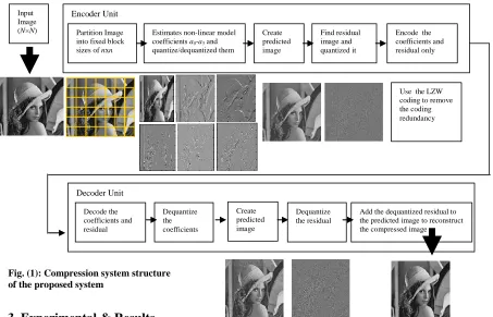
The steps below illustrate clearly the implementation of proposed system in details, the system layout shown in Figure (1):
Step 1: Load the original uncompressed gray image G of BMP format of size N×N.
Step 2: Partition the image G into nonoverlapping square fixed block of size n×n, then compute the estimated coefficients of the extended nonlinear model according to equations below, by first finding the a1,
a2and a5 coefficients, such as:
) 1 ...( ... ) ( ) )( , ( 1 0 1 0 2 1 0 1 0 1 n x n y n x n y xc x xc x y x G a
) 2 ...( ... ) ( ) )( , ( 1 0 1 0 2 1 0 1 0 2 n x n y n x n y yc y yc y y x G a
) 3 ...( ... ) ( ) ( ) )( )( , ( 1 0 1 0 2 2 1 0 1 0 5
n x n y n x n y yc y xc x yc y xc x y x G a ) 4 ...( ... ... 2 1 yc n xcWhere xc equal to yc that represents a block centre of size (n×n).
For the coefficients a0,a3 and a4, the extended approximation polynomial mode can be summarized as:
) 7 ....( ... ) 6 ...( ... ) 5 ...( ... 3 4 4 3 2 0 3 4 4 3 3 2 0 2 2 4 2 3 1 0 1 W a W a W a V W a W a W a V W a W a W a V 1 0 1 0 2 2 4 1 0 1 0 4 4 3 1 0 1 0 2 2 2 1 ) 11 ...( ... ... ) ( ) ( ) 10 ...( ... ) ( ) ( ) 9 ...( ... ) ( ) ( ) 8 ( ... ... ... ... ... ... n x n y n x n y n x n y yc y xc x W yc y xc x W yc y xc x W n n W Where
) 12 ...( ... ... ) , ( 1 0 1 0 1
n x n y y x G
V
1 0 1 0 2
2 n ( ) (, )...(13)
x n y y x G xc x
V
1 0 1 0 2
3 n ( ) (, )...(14) x n y y x G yc y V
In order to find the required coefficients, apply the Crammers rule, where:
) 15 ....( ... W W W W W W W W W W W W 3 4 2 4 3 2 2 2 1 3 4 3 4 3 2 2 2 1 0 W W W V V V
a
...(16)
W W W W W W W V W V W V 3 4 2 4 3 2 2 2 1 3 3 2 4 2 2 2 1 1 3 W W W W W W
a ...(17)
Here in the nonlinear form, the polynomial representation approximation model required 6 coefficients to represents each block compared to the linear model that require 3 coefficients. Basically, the nonlinear based needs times two of linear model coefficients, in spite of that, the compression performance not affected by these additional coefficients since the residual decrease due to increase the modelling efficiency. The main reason of estimating the coefficients decorrelation or removing of interpixel (spatial) redundancy (interpixel) is possible, by using the modelling concept.
Step 3: Quantize the estimated coefficients from step above using the popular scalar uniform quantizer, simply by dividing the each of the computed coefficients by the quantization step to eliminate the psychovisual redundancy. Here 3 quantization level of values required according to coefficients importance, one for a0 values, other one for the a1 & a2 and the last one for a3,a4 &a5 values. The quantizer/dequantizer as shown in equations (18-23).
) 23 ...( ) ( ) 22 ...( ) ( ) 21 ...( ) ( ) 20 ...( ) ( ) 19 ( ... ) ( ) 18 ...( ... ) ( 2 2 2 2 2 2 1 1 1 1 5 5 5 5 4 4 4 4 3 3 3 3 2 2 2 2 1 1 1 1 0 0 0 0 0 0 a a a a a a a a a a a a QS Q a D a QS a round Q a QS Q a D a QS a round Q a QS Q a D a QS a round Q a QS Q a D a QS a round Q a QS Q a D a QS a round Q a QS Q a D a QS a round Q a
Where QSa0 quantization step of a
0 coefficient,
1
a
QS quantization step of a1 & a2 coefficients and
2
a
QS quantization step
of a3, a4 & a5 coefficients.
Step 4: Create the predicted image G~ as a nonlinear combination polynomial model of dequantized coefficients and pixel distance
) 24 )...( ).( ( ) ( ) ( ) ( ) ( ~ 5 4 3 2 1 1 0 2
2 a y yc a x xc y yc
xc x a yc y a xc x a W a
G
The predicted image G~corresponds to the modelled image representation that similar to the original image one, which is a weighted sum of coefficients and the pixel distance.
Step 5: Find the residual (prediction error) as a difference between original uncompressed image G and the predicted image G~
) 25 ...( ... ... ... ~ ResGG
The residual represents the information lost which can not be predicted accurately since the image features or characteristics cannot usually be fully described by a model where the details vary from part to part. The residual image acts as a quality indicator or measure of fit for the model, where a smaller residual indicates high compression gain, due to the adequate prediction model, while a larger residual indicates a low compression gain due to a poor prediction model [9].
Step 6: Quantize the residual image as in step 3 using the simple scalar uniform quantizer/dequantizer, such as: ) 26 ...( ... ... Re Re ) Re ( Re Re
Res s
QS sQ sQD QS s round
sQ
Where QSRe quantization step of residual image.s
Step 7: Encode the lossily quantized information of estimated coefficients and residual image using the LZW coding to eliminate/remove the coding redundancy by converting them into variable bit length coding. The decoder reconstructs the compressed image Gˆ using only the information decoded of coefficients and
residual, where the dequantized coefficients utilized to create the predicted image (see eq. 24), and then added to the dequantized residual image, such that:
) 27 ....( ... ... ... ... ... Re ~
ˆ G sQD
3. Experimental & Results
In general, as a lossy compression system utilized, the performance measure based on the objective fidelity criteria of Peak Signal to Noise Ratio (PSNR) (see equation 28 ), along with the Compression Ratio (CR) (see equation 29). Here various standard images were selected that characterized by variation in details, where the complex selected image of highly details such as Baboon (see figure 2a), the less complex one of medium details such as Lena (see figure 2b), and the simple image of small details such as Woman (see figure 2c), all the images are square gray scale images of size 256x256 pixels of 8 bit/per pixel.
(ˆ( , ) ( , )
...(28)1
255 log
. 10
1
0 1
0
2 2
10
N
x N
y
y x I y x I N
N PSNR
) 29 ...( ... ... ... Im
rmation ressedInfo SizeofComp
age inal SizeofOrig nRatio
Compressio
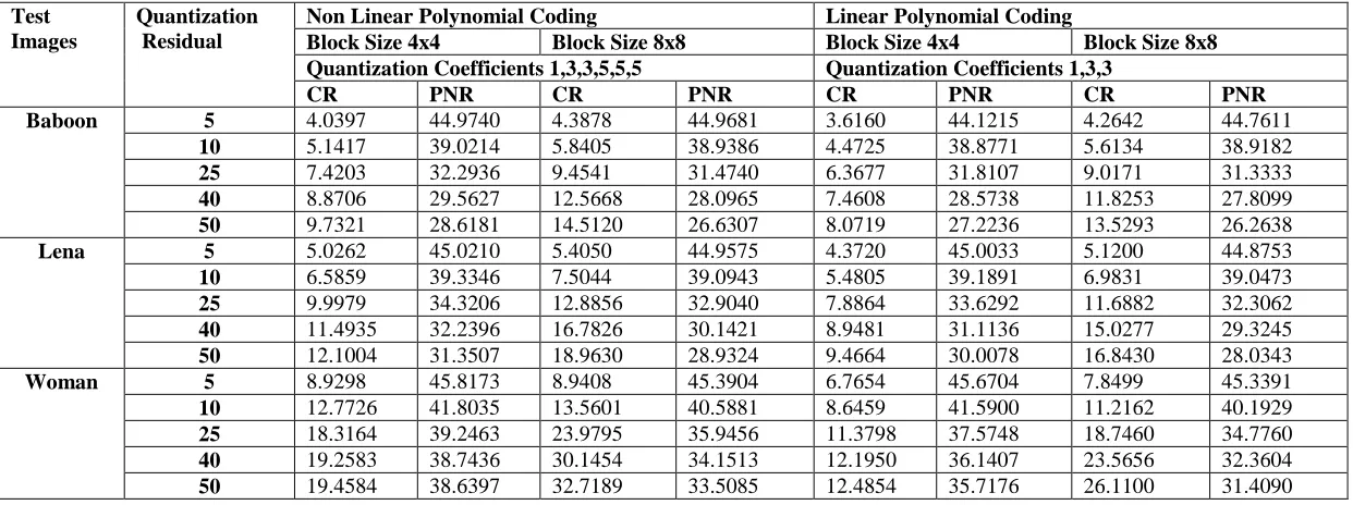
Table (1) illustrated the comparison performance of both linear and nonlinear polynomial coding techniques on the tested images, using two blocks of sizes 4×4 and 8×8, with quantization levels of coefficients of linear base equals to 1,3,3 and nonlinear base equals to 1,3,3,5,5,5, and with different quantization levels of residual image.
The results clearly showed the higher performance of nonlinear model base in terms of compression ratio and the quality that due to involving more coefficients of nonlinear terms where more accurately estimated the predicted image which leads to less residual error compared to the linear base model. Also the techniques of linear and nonlinear base implicitly affected by the block size and the quantization levels of the residual image, where for bigger block sizes and/or higher quantization levels higher compression achieved with lower PSNR quality image, and vice versa. Lastly, the results vary according to image details, where for the simple images more compression achieved compared to highly detailed image of low
Input Image (N×N)
Encoder Unit
Partition Image into fixed block sizes of nxn
Estimates non-linear model coefficients a0-a5 and
quantize/dequantized them
Create predicted image
Find residual image and quantized it
Encode the coefficients and residual only
Decoder Unit
Dequantize the coefficients
Add the dequantized residual to the predicted image to reconstruct the compressed image Create
predicted image Decode the
coefficients and residual
Dequantize the residual
Use the LZW coding to remove the coding redundancy
Fig(2): Tested images
a b c
a b
c
Table (1): Comparison performance between linear and non-linear polynomial coding techniques, using two blocks of sizes 4×4 and 8×8, with quantization levels of coefficients of linear base equals to 1,3,3 and nonlinear base equals to 1,3,3,5,5,5, and with different quantization levels of residual image.
Test Images
Quantization Residual
Non Linear Polynomial Coding Linear Polynomial Coding
Block Size 4x4 Block Size 8x8 Block Size 4x4 Block Size 8x8 Quantization Coefficients 1,3,3,5,5,5 Quantization Coefficients 1,3,3
CR PNR CR PNR CR PNR CR PNR
Baboon 5 4.0397 44.9740 4.3878 44.9681 3.6160 44.1215 4.2642 44.7611
10 5.1417 39.0214 5.8405 38.9386 4.4725 38.8771 5.6134 38.9182
25 7.4203 32.2936 9.4541 31.4740 6.3677 31.8107 9.0171 31.3333
40 8.8706 29.5627 12.5668 28.0965 7.4608 28.5738 11.8253 27.8099
50 9.7321 28.6181 14.5120 26.6307 8.0719 27.2236 13.5293 26.2638
Lena 5 5.0262 45.0210 5.4050 44.9575 4.3720 45.0033 5.1200 44.8753
10 6.5859 39.3346 7.5044 39.0943 5.4805 39.1891 6.9831 39.0473
25 9.9979 34.3206 12.8856 32.9040 7.8864 33.6292 11.6882 32.3062
40 11.4935 32.2396 16.7826 30.1421 8.9481 31.1136 15.0277 29.3245
50 12.1004 31.3507 18.9630 28.9324 9.4664 30.0078 16.8430 28.0343
Woman 5 8.9298 45.8173 8.9408 45.3904 6.7654 45.6704 7.8499 45.3391
10 12.7726 41.8035 13.5601 40.5881 8.6459 41.5900 11.2162 40.1929
25 18.3164 39.2463 23.9795 35.9456 11.3798 37.5748 18.7460 34.7760
40 19.2583 38.7436 30.1454 34.1513 12.1950 36.1407 23.5656 32.3604
References
1- Gonzalez, R. C. and Woods, R. E. 2003. Digital Image Processing 2nd edn. Prentice Hall.
2- Sayood, K. Introduction to Data Compression. 2006. 3rd edn.Elsevier Inc., San Francisco United States of America.
3- Sachin, D. 2011. A Review of Image Compression and Comparison of its Algorithms. International Journal of Electronics & Communication Technology, 2(1), 22-26.
4- Asha, L. and Permender, S. 2013. Review of Image Compression Techniques. International Journal of Technology and Advanced Engineering, 3(7),461-464.
5- Asolkar, P. S., Zope, P. H. and Suralkar S. R. 2013. Review of Data Compression and Different Techniques of Data Compression. International Journal of Engineering Research & Technology, 2(1), 1-8. 6- Amruta, S.G. and Sanjay L.N. 2013. A Review on Lossy to Lossless Image Coding. International Journal of Computer Applications , 67(17), 9-16.
7- Vijayvargiya, G., Silakar,i S. and Pandey R. 2.13. A Survey: Various Techniques of Image Compression, International Journal of Computer Science and Information Security, 11(10),51-55.
8- Khobragede, P. and Thakare, S. 2014. Image Compression Techniques-A Review International Journal of Computer Science and Information Technologies, 5(1),272-275.
9- Ghadah, Al-K. 2012. Intra and Inter Frame Compression for Video Streaming. Ph.D. thesis, Exeter University, UK.
10- Tang, H. and Kamata, S-I. 2006. A Gradient Based Predictive Coding for Lossless Image Compression. IEICE Transactions on Information and Systems, E89-D(7), 2250-2256.
11- Avramović, A. and Savić, S. 2011. Lossless Predictive Compression of Medical Images. Serbian Journal of Electrical Engineering, 8(1), 27-36.
12- Ghadah, Al-K. 2013. Hierarchal Autoregressive for Image Compression. The Proceeding of the 4th Conference of College of Education for Pure Science, Thi-Qar University, 4(1), 235-241.
13- George, L. E. and Sultan, B. 2011. Image Compression Based on Wavelet, Polynomial and Quadtree. Journal of Applied Computer Science & Mathematics, 11(5), 15-20.
14- Ghadah, Al-K. and George, L. E..2013.Fast Lossless Compression of Medical Images based on Polynomial. International Journal of Computer Applications, 70(15), 28-32.
15- Ghadah, Al-K. 2013. Image Compression based on Quadtree and Polynomial. International Journal of Computer Applications (IJCAs), 76(3),31-37.
16- Ghadah, Al-K. and Haider, Al-M. 2013. Lossless Compression of Medical Images using Multiresolution Polynomial Approximation Model. International Journal of Computer Applications, 76(3),38-42.
17- Ghadah, Al-K. 2013. Hybrid Image Compression based on Polynomial and Block Truncation Coding. Electrical, Communication, Computer, Power, and Control Engineering (ICECCPCE), 2013, International Conference on Mosul, IEEE.
18- Ghadah, Al-K and Hazeem, Al-K, 2014. Medical Image Compression using Wavelet Quadrants of Polynomial Prediction Coding & Bit Plane Slicing. International Journal of Advanced Research in Computer Science and Software Engineering, 4(6), 32-36.
19- Ghadah, Al-K. 2014. Wavelet Transform and Polynomial Approximation Model for Lossless Medical Image Compression. International Journal of Advanced Research in Computer Science and Software Engineering. 4(3), 584-587.
20-Rasha, Al-T, and G. and Ghadah, Al-K. 2015. Image Compression using Hierarchal Linear Polynomial Coding, International Journal of Computer Science and Mobile Computing, 4(1), 112-119.