A Review on LBG Algorithm for Image
Compression
Ms. Asmita A.Bardekar#1, Mr. P.A.Tijare#2
#
CSE Department, SGBA University, Amravati. Sipna’s College of Engineering and Technology,
In front of Nemani Godown Badnera Road, Amravati, Maharashtra, India
Abstract-One of the important factors for image storage or transmission over any communication media is the image compression. Compression makes it possible for creating file sizes of manageable, storable and transmittable dimensions. Compression is achieved by exploiting the redundancy. Image Compression techniques fall under two categories, namely, Lossless and Lossy. The Algorithm, used for this purpose, is the Linde, Buzo, and Gray (LBG) Algorithm. This is an iterative algorithm which alternatively solves the two optimality criteria i.e. Nearest neighbor condition and Centroid condition . The algorithm requires an initial codebook to start with. Codebook is generated using a training set of images. The set is representative of the type of images that are to be compressed. There are different methods like Random Codes and Splitting in which the initial code book can be obtained. This initial codebook is obtained by the splitting method in LBG algorithm. In this method an initial code vector is set as the average of the entire training sequence. This code vector is then split into two. The iterative algorithm is run with these two vectors as the initial codebook. The final two code vectors are splitted into four and the process is repeated until the desired number of code vector is obtained. The compression algorithm can be measured by certain performances such as Compression Ratio (CR), Peak Signal-to-Noise Ratio (PSNR).
Keywords- Vector quantization, Codebook generation, LBG
algorithm, Image compression.
I. INTRODUCTION
In this paper, the LBG algorithm for image compression is reviewed. One of the important factors for image storage or transmission over any communication media is the image compression. Compression makes it possible for creating file sizes of manageable, storable and transmittable dimensions. Compression is achieved by exploiting the redundancy. Image Compression techniques fall under two categories, namely, Lossless and Lossy. In Lossless Techniques the image can be reconstructed after compression, without any loss of data in the entire process. Lossy techniques, on the hand are irreversible, because, they involve performing quantization, which result in loss of data. More compression is achieved in the case of lossy compression than lossless compression[2].In return for accepting this distortion in the
blocks [6].Vector Quantization (VQ) methods allow arbitrary compression of digital images. They are widely employed in encoding video. These methods share a common structure. The image is divided into pixel blocks and these blocks are approximated by a smaller set of images drawn from a fixed code book. The number of bits needed to specify the original code block is replaced by the typically smaller number of bits needed to specify its corresponding code. The image compression using vector quantization (VQ) techniques has received large interest .In VQ approaches adjacent pixels are taken as a single block, which is mapped into a finite set of codewords. In decoding stage the codewords are replaced by corresponding vectors. The set of codewords and the associated vectors together is called a codebook. In VQ, the correlation which exists between adjacent pixels are naturally taken into account, and with a comparatively small codebook one achieves a small quantization error in reconstructed images. The main idea in VQ, is to find a codebook which minimizes the quantization mean error in reconstructed images. One of the best known VQ methods is the Linde-Buzo-Gray (LBG) algorithm, which iteratively searches clusters in the training data. The cluster centroids are used as the codebook vectors, while the codewords for them can be selected arbitrarily [10].The compression rate is the ratio of the file size of the uncompressed image over the size for the compressed image, denoted. The compression rate is varied by decreasing the size of the codebook but typically at the cost of increasing the discrepancy between a block and the code which replaces it.
II.RELATED WORK
Grouping source outputs together and encoding them as a single block, we can obtain efficient lossy as well as lossless compression algorithms. We can view blocks as vectors, hence the name “vector quantization”. Vector Quantization (VQ) is a lossy data compression method based on the principle of Block Coding. It is a fixed- to- fixed length algorithm .The design of the vector quantizer (VQ) is considered to be a challenging problem due to the need for multi-dimensional integration [3]. Linde, Buzo and Gray (LBG) proposed a VQ design algorithm based on a training sequence.The use of the training sequence bypasses the need for multidimensional integration [1].Each quantizer codeword represents a single sample of the source output. By taking longer and longer sequences of input samples, it is possible to extract the structure in the source coder output. Even when the input is random, encoding sequences of samples instead of encoding individual samples separately provides a more efficient code. Encoding sequences of samples is more advantageous in the lossy compression framework as well. By “advantageous” we mean a lower distortion for a given rate, or a lower rate for a given distortion. By “rate” we mean the average number of bits per input sample, and the measures of distortion will generally be the mean squared error and the signal-to-noise ratio. The idea that, encoding sequences of outputs can provide an advantage over, the encoding of individual samples and the basic results in information theory
were all proved by taking longer and longer sequences of inputs. This indicates that a quantization strategy that works with sequences or blocks of output would provide some improvement in performance i.e. if we wish to generate a representative set of sequences.
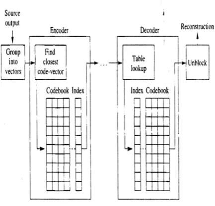
Given a source output sequence, we would represent it with one of the elements of the representative set. In vector quantization we group the source output into blocks or vectors. For example, we can take a block of L pixels from an image and treat each pixel value as a component of a vector of size or dimension L. This vector of source outputs forms the input to the vector quantizer. The encoder and decoder of the vector quantizer, we have a set of L-dimensional vectors called the codebook of the vector quantizer. The vectors in this codebook, known as code-vectors are selected to be representative of the vectors we generate from the source output. Each code-vector is assigned a binary index. At the encoder, the input vector is compared to each code-vector in order to find the code-vector closest to the input vector. In order to inform the decoder about which code-vector was found to be the closest to the input vector, we transmit or store the binary index of the code-vector. Because the decoder has exactly the same codebook, it can retrieve the code-vector given its binary index. A pictorial representation of this process is shown in Fig.1
Fig. 1 The vector quantization procedure
compression, the goal of vector quantization, can then be achieved by transmitting or storing only the index of the vector.
The most commonly Known and used algorithm is the Linde-Buzo-Gray (LBG) algorithm. Codebook Initialization has methods, they are random codes, which use a random initial codebook where the first Nc, vectors (or any widely spaced Ncvectors) of the training set are chosen as the initial codebook and in splitting centroids for the entire training set is found, and this single codeword is then split (perturbed by a small amount) to form two codewords. Design continues, optimum code of one stage is split to form an initial code for the next stage until Nc code vectors are generated.
For a particular training set (e.g. training set corresponding to approximate component) a step by step selection process is applied to generate a prescribed number of temporary clusters. ‘Similar' vectors of the training space gather under the same cluster. Clustering process is initiated by finding the smoothest vector in the training space. The variance of a vector is used as the determining factor of smoothness and the vector having minimum variance is selected as the smoothest vector and termed as the reference vector. From these clusters, C vectors are chosen very carefully, one from each cluster, by natural selection. The quality of reconstructed image depends on the level of decomposition and size of the codebook. It also depends on the code vector dimension .More the size of the codebook, better the quality, but it correspondingly increases the rate. The amount of compression will be described in terms of the rate, which will be measured in bits per sample. Suppose we have a codebook of size K, and the input vector is of dimension L. In order to inform the decoder of which code-vector was selected, we need to uselog K2 bits. For example, if the codebook
contained 256 code-vectors, we would need 8 bits to specify which of the 256 code-vectors had been selected at the encoder. Thus, the number of bits per vector is log K2 bits. As each code-vector contains the reconstruction values for L, source output samples, the number of bits per sample would be
2
log K
/L. Thus, the rate for an L-dimensional vector quantizer with a codebook of size K is log K2 /L. When we
say that in a codebook C containing the K code-vectors {Yi} , the input vector X is closest to Yj we will mean that
||X-Yj||2
≤
||X-Yi||2 for all Yi
C ,Where X = (x1 x2…xL) And ||X||2 = 2
1
x
L i iWhen we are discussing compression of images, a sample refers to a single pixel. Finally, the output points of the quantizer are often referred to as levels. Thus, when we wish to refer to a quantizer with K output points or code-vectors, we may refer to it as a K-level quantizer. As we block the input into larger and larger blocks or vectors, these higher
of the smaller codebook into two. The size of the codebook is always in powers of two (2M → 2(M+1)). Hence, relatively similar two image blocks may have same closest match codeword in Jth position at codebook of size 2M and at codebook of size 2(M+1), one of the two image blocks may have its closest match codeword at Jth place in the codebook and other block’s codeword may be in (J+1)th place[9]. Thus, the quantizer is completely defined by the output points and a distortion measure. The main problem in VQ is choosing the vectors for the codebook so that the mean quantization error is minimal, after the codebook is known, mapping input vectors to it is a trivial matter of finding the best match. As earlier VQ compression requires ¼ codebook entry of total length blocks if we select 2x2 block size , and index finding time is more as the codebook entry is more ,so it is not suitable for the fast data transaction . Codebook formulation is also requires more time while LBG is efficient and very good choice for data transmission as it uses minimum codebook entries. Again it also need codebook entries and that has to formulate fast with minimum block size .The major problem is the length of codebook and time require to formulate the codebook .We have to make balancing between length of codebook entries, block size selection and time required to formulate the codebook. The maximum entries in the codebook will be time consuming. Then we should have initial codebook having some decided entries if the codebook entry does not match with initial codebook it will have more distortion. So, we have LBG algorithm which is optimize.
III. LBG ALGORITHM
The Linde, Buzo, and Gray (LBG) Algorithm, is an iterative algorithm which requires an initial codebook to start with. Codebook is generated using a training set of images [5].The set is representative of the type of images that are to be compressed. There are different methods like Random Codes and Splitting [4], in which the initial code book can be obtained. This initial codebook is obtained by the splitting method in LBG algorithm. In this method an initial code vector is set as the average of the entire training sequence. This codevector is then split into two. The iterative algorithm is run with these two vectors as the initial codebook. The final two codevectors are splitted into four and the process is repeated until the desired number of code vectors is obtained[1].The compression algorithm can be measured by certain performances such as compression Ratio(CR),Peak Signal to Noise ratio(PSNR)[2].
One way of exploiting the structure in the source output is to place the quantizer output points where the source output (blocked into vectors) are most likely to congregate. The set of quantizer output points is called the codebook of the quantizer and the process of placing these output points is often referred to as codebook design. When we group the source output in two-dimensional vectors, we might be able to obtain a good codebook design by plotting a representative set of source output points and then visually locate where the quantizer output points should be. However, this approach to codebook design breaks down when we design
higher-dimensional vector quantizer. So we need an automatic procedure for locating where the source outputs are clustered [7].Linde-Buzo and Gray algorithm is as follows.
1. Start with an initial set of reconstruction values
( )1
M o
i i
Y
. Set k = 0, D
(0) = 0. Select threshold
. (Forpractical implementation we truncate step 1 as set of training vectors =
X
n n 1N , where N = new value of total training vectors.)2. Find quantization regions
( )k
: ( , )
( , )
i i j
V
X d X Y
d X Y
j
i
j = 1, 2,…, M. 3. Compute the distortion,
( )
2
( ) ( )
1
( )
k
i
M
k k
i X
V i
D
X
Y
f
X dX
4. If
(k) (k 1)
(k)
(D
D
)
D
, stop; otherwise, continue.
5. k= k+1. Find new reconstruction values
( ) 1M k
i i
Y
that
are the centroids of
(k 1)
iV
. Go to Step 2.This algorithm forms the basis of most vector quantizer designs. It is popularly known as the Linde-Buzo-Gray or LBG algorithm. Linde, Buzo and Gray described a technique called splitting technique for initializing the design algorithm. We begin by designing a vector quantizer with a single output point, in other words, a codebook of size one, or a one-level vector quantizer. With a one-element codebook, the quantization region is the entire input space, and the output is the average value of the entire training set. From this output point ,the initial codebook for a two-level vector quantizer can be obtained by including the output point for the one-level quantizer and a second output point obtained by adding a fixed perturbation vector
. We then use the LBG algorithm to obtain the two-level vector quantizer. Once the algorithm has converged, the two codebook vectors are used to obtain the initial codebook for a four-level vector quantizer. This initial four- level codebook consists of the two codebook vectors from the final codebook of the two-level vector quantizer and another two vectors obtained by addingconvergence of the algorithm depends on the initial conditions. So a splitting technique has been used for initializing the design algorithm. A one-level vector quantizer is designed with a code book of size one, which is the average of all the training vectors in the set. The initial codebook for a two-level vector quantizer is obtained by retaining the original output, and the second one obtained by adding a fixed perturbation vector
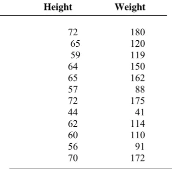
to it. After convergence, the two-level VQ is used to yield a four-two-level VQ in a similar manner. The above procedure is repeated till a codebook of required size is obtained. The codebook size increases exponentially with the rate of the quantizer, increasing the size of the codebook increases the quality of the reconstruction, but the encoding time also increases due to the increase in the computations required to find the closest match. By including the final codebook of the previous stage at each splitting, we guarantee that the codebook after splitting will be at least as good as the codebook prior to splitting. In order to see how this algorithm functions, consider the following example of a two-dimensional vector quantizer codebook design [7].Example: Suppose our training set consists of the height and weight values shown in Table 1. The initial set of output points is shown in Table 2 (For ease of presentation, we will always round the coordinates of the output points to the nearest integer.) The inputs, outputs, and quantization regions are shown in Fig.2
TABLE 1
TRAINING SET FOR DESIGINING VECTOR QUANTIZER CODEBOOK
Height Weight
72 180
65 120
59 119
64 150
65 162
57 88
72 175
44 41
62 114
60 110
56 91
70 172
TABLE 2 INITIAL SET OF OUTPUT POINTS FOR CODEBOOK DESIGN Height Weight 45 50
75 117
45 117
80 180
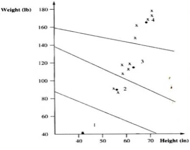
The input (44, 41) has been assigned to the first output point; the inputs (56, 91), (57, 88), (59, 119), and (60, 110) have been assigned to the second output point: the inputs (62, 114), and (65, 120) have been assigned to the third output, and the five remaining vectors from the training set have been assigned to the fourth output. The distortion for this assignment is 387.25. We now find the new output points. There is only one vector in the first quantization region, so the first output point is (44, 41). The average of the four vectors in the second quantization region (rounded up) is the vector (58,102), which is the new second output point. In a similar manner, we can compute the third and fourth output points as (64, 117) and (69, 168). The new output points and the corresponding quantization regions are shown in Fig. 3. From Fig. 3 we can see that, while the training vectors that were initially part of the first and fourth quantization regions are still in the same quantization regions, the training vectors (59,115) and (60,120), which were in quantization region 2, are now in quantization region 3. The distortion corresponding to this assignment of training vectors to quantization regions is 89, considerably less than the original 387.25. Given the new assignments, we can obtain a new set of output points. The first and fourth output points do not change because the training vectors in the corresponding regions have not changed. However, the training vectors in regions 2 and 3 have changed. Recomputing the output points for these regions, we get (57, 90) and (62, 116). The final form of the quantizer in shown in Fig.4. The distortion corresponding to the final assignments is 60.17[7].
Fig. 2 Initial state of the vector quantizer
Fig. 4 Final state of the vector quantizer
The LBG algorithm guarantees that the distortion from one iteration to the next will not increase [7] .This compression is measured by certain performances such as Compression Ratio (CR), Peak Signal-to-Noise Ratio (PSNR)[2] .Compression Ratio (CR), is defined as a ratio of the number of bits required to represent the data before compression to the number of bits required after compression. Mean square error (MSE), refers to the average value of the square of the error between the original signal and the reconstruction. A common measure of distortion is the mean squared error (MSE). Peak Signal-to-Noise Ratio (PSNR),is defined as the ratio of square of the peak value of the signal to the mean square error. The distortion in the decoded images measured using peak signal-to-noise ratio (PSNR)[10].
IV. APPLICATION
Data transfer of uncompressed image over digital networks requires very high bandwidth .The state-of-the-art image compression techniques may exploit the dependencies between the sub-bands in a transformed image. The LBG algorithm reduces complexity of a transferred image without sacrificing performance. The image compression have diverse applications including Tele-video-conferencing, Remote sensing, document and Medical imaging etc.
V. CONCLUSION
With this review, we came to the conclusion that Linde, Buzo and Gray (LBG) algorithm reduces complexity of a transferred image without sacrificing performance by splitting technique for the codebook generation.
REFERENCES
[1] Y.Linde,A.Buzo,and R.M.Gray, ”An Algorithm forVector Quantizer Design”, IEEE Transactions on Communications ,January 1980.
[2] A.Vasuki and P.T.Vanathi, ”Image Compression using Lifting and Vector Quantization”, GVIP Journal Volume 7, Issue 1,April 2007.
[3] P. Franti , "Genetic algorithm with deterministic crossover for vector quantization", Pattern Recognition Letters, 21 (1), 61-68, 2000.
[4] P.Franti, T.Kaukoranta, D.-F.Shen and K.-S.Chang, "Fast and memory efficient implementation of the exact PNN", IEEE Transactionsons Image Processing,9 (5), 773-777,May 2000.
[5] Qin Zhang, John M.Danskin, Neal E.Young,”A codebook generation algorithm for document image compression,6211 Sudikoff Laboratory,Department Computer Science, Dartmouth College, Hanover,USA.
[6] Yu-chen Hu,Bing-Hwang Su,Chih-Chiang Tsou.”Fast VQ codebook search algorithm for grayscale imagecoding”,ScienceDirect,Image and vision computing 26(2008) 657-666.
[7] Khalid Sayood,”Introduction to Data Compression”,Harcourt India Private limited,New Delhi.
[8] Robert D. Dony, ”Neural Network Approaches to Image Compression”, IEEE Simon Haykin, IEEE, Proceeding of the IEEE, vol. 83,no.2,
February 1995.
[9] K.Somasundaram, and S.Domnic ,“Modified Vector Quantization Method for Image Compression”, World Academy of Science, Engineering and Technology 19 2006.
![Bis{1 [2 (diphenylphosphino)ethyl] 3 ethylimidazol 2 ylidene}palladium(II) bis(hexafluoridophosphate) acetonitrile 2 85 solvate](data:image/gif;base64,R0lGODlhAQABAIAAAP///wAAACH5BAEAAAAALAAAAAABAAEAAAICRAEAOw==)