Spatial temporal analysis of the distribution of pediatric tuberculosis patterns in Kenya

(1)

Kiplimo Richard Kibet REG. NO. I56/CTY/PT/21419/2010

(2)

DECLARATION

I declare that this thesis is my own work and it has not been presented in any other university for an award of a degree.

Signature……… Date………

Kiplimo Richard Kibet

This thesis has been submitted for examination with our approval as University Supervisors.

Signature: ……….. Date: ………

Dr. Gachangi Njenga

Kenyatta University, Nairobi, Kenya

Signature: ……….. Date: ………...

Mr. Hillary Kipruto

(3)

DEDICATION

(4)

ACKNOWLEDGEMENT

My special, deepest and sincere appreciation goes to my supervisors, Dr. Gachangi Njenga and Hillary Kipruto whose initial encouragement and subsequent support and supervision shaped my thinking and gave me more insight into the completion of this project. Their thinking and

suggestions greatly influenced my view of the research problem and led to the successful

completion.

I also acknowledge the Division of Leprosy Tuberculosis and Lung Disease for availing the data for this study and more so giving me an opportunity to serve as an intern at the division during

this time. This gave me an insight understanding of tuberculosis.

Lots of thanks go to all my lecturers and the academic staff of Department of Mathematics,

Kenyatta University for their dedicated training in all aspects of Biostatistics.

I also appreciate my aunt Leah Rotich, Cousins and friends Kazi David, Gilbert Sang and Gershom Richard for their advice and material support during the study period.

Finally, my most profound thanks to God my faithful shepherd.

(5)

LIST OF TABLES

Table 4.2: Summary Table of the Global Moran‟s I output results for year 2010 ... 28

Table 4.3: Summary Table of the Global Moran‟s I output results for year 2011 ... 29

(9)

LIST OF FIGURES

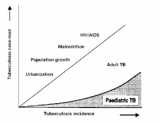
Figure 1.1: Schematic illustration of the increasing proportion of the TB case-load comprising children as total TB incidence increases. ... 3

Figure 4.1: A graph showing the number of pediatric cases and the incidence rate per 100, 000 for the years 2009, 2010 and 2011……….. 24

Figure 4.2 A graph showing the incidence rate of pediatric TB for the three years per 100,000 population……….24

Figure 4.3: A graph showing the different types of tuberculosis in children (in percentage)………..25

Figure 4.4: A graph showing five counties with the highest population and six with the lowest population……….25

Figure 4.5: Graphs showing the distribution of the pediatric cases in the various counties for the three years of study………... 26

Figure 4.6 Choropleth maps (a), (b) and (c) showing the distribution of incidence of pediatric TB cases over the study region for the years 2009, 2010 and 2011 respectively………31

Figure 4.7: A snipped map showing the area with highest incidence for the year 2009………. 32

Figure 4.8: A choropleth map showing statistical significant relationship between counties and their

neighbours in the year 2009 33

(10)

Figure 4.11: A map showing the hot spot areas in the year 2009……… 38

Figure 4.12: A map showing the hot spot areas in the year 2010……… 39

(11)

ACRONYMS

AND

ABBREVIATIONS

AFB Acid Fast Bacilli

AIDS Acquired Immune Deficiency Syndrome

BCG Bacille Calmette-Guérin

DLTLD Division of Leprosy, Tuberculosis and Lung Disease

DOTS Direct Observe Therapy Strategy

DTLC District Tuberculosis and Leprosy Coordinator

EPTB Extra Pulmonary Tuberculosis

GIS Geographical Information Systems

HIV Human Immune Virus

LTBI Latent Tuberculosis Infection

MCMC Markov Chain Monte Carlo

MDR-TB Multi-drug-resistant tuberculosis

MPS Multiple-Point Geo-statistics

(12)

TB Tuberculosis

TDR-TB Total-drug-resistant tuberculosis

WHO World Health Organization

(13)

ABSTRACT

(14)

(15)

CHAPTER ONE INTRODUCTION

1.1 Background

Tuberculosis is a leading cause of mortality and morbidity globally Dirk et al. (2008). Among

children, it is a top 10 cause of death (Rekha, 2010). However from the article “global overview and challenges of TB”, children with TB are given low priority in most national health programs

and are neglected in this epidemic. This is because from a TB control point of view, they rarely

transmit the disease and contribute little to the maintenance of the TB epidemic. However, children do contribute a substantial proportion of the global TB disease burden, (Society, 2012).

Of the 1 million estimated cases of TB in children worldwide, 75% occur in the 22 high-burden countries (Rekha, 2010). Kenya is among the 22 listed countries and is ranked number 15 worldwide while in Africa, it is ranked number five (USAID, 2009). In fact, there are an

estimated 12,000 TB-infected children younger than 14, representing 11 percent of all infections (IRIN, 2012).

TB disease in adults comprises a combination of recent infections and reactivation of latent TB, and therefore represents both recent and past TB exposure Dirk et al. (2008). HIV co-infection

increases the progression to disease of both recent and latent TB infection. According to Dirk et al. (2008), childhood infection is acquired predominantly from adults; as child-to-child transmission is uncommon and young children with TB infection have a greater risk for

(16)

Vaccination has been the primary TB prevention method in children (Sandoz, 2006). In fact, the journal “Doctors Section” shows BCG vaccine as the most widely used vaccine in the world.

Although it protects against disseminated and severe forms of the disease in young children, its safety in the HIV-infected population has been questioned (Sandoz, 2006). Also, a quarter of a

million children still develop TB every year: Particularly vulnerable to infection from household contacts, many of them have been infected in their own homes, by parents or other relatives with

active, infectious TB.

A major challenge of childhood TB is establishing an accurate diagnosis. This has been notoriously difficult, as the early symptoms and signs are easily missed. Also, young children

suffer more extra pulmonary and disseminated TB than adults. Lastly, treatment of TB in children is challenging due to the lack of pediatric drug formulations and challenges in

monitoring of toxicity (Loeffler, 2003).

The importance of pediatric TB must be stressed for several reasons. First, untreated children with LTBI serve as the pool for future TB epidemics i.e. a percentage of children with LTBI

eventually will reactivate their infection and develop active TB (Loeffler, 2003). Also, young children are especially vulnerable because if infected, they are more likely than adults to develop

active and disseminated TB. These forms need to be recognized and treated early to avoid significant morbidity and mortality.

(17)

low, there is a significant increase with increasing cases in the adults. Also, the graph

demonstrates that the risk factors include HIV/AIDS, malnutrition, population growth and urbanization.

Figure 1.1: Schematic illustration of the increasing proportion of the TB case-load comprising children as total TB incidence increases.

1.1.1 Transmission, Diagnosis, Prevention and Treatment

Transmission of TB occurs when an individual with active pulmonary TB cough, sneeze, speak,

(18)

(Rekha, 2010). "GeneXpert," which was recently announced and certified by the WHO gives a

great opportunity with diagnostic as it can give a 30% more accurate result of whether a person has TB than current tests (Motsoaledi, 2011). Prevention and control of TB primarily rely on screening programs and vaccination of infants, usually with BCG vaccine (DLTLD, 2012).

From (DLTLD, 2012), the recommended treatment of new onset pulmonary TB as of the year 2010 is six months of a combination of antibiotic containing rifampicin along isoniazid,

pyrazinamide and ethambutol for the first two months and with just isoniazid for the last four months.

1.1.3 Risk Factors

There are a number of risk factors that make people more susceptible to TB infections.

Worldwide the most important of these is HIV with co-infection present in about 13% of cases Wikipedia (2012, Jan 17). This is a particular problem in Sub-Saharan Africa where rates of HIV are high but we are hopeful that the control of HIV in the future will check this resurgence of

TB. It is closely linked to both overcrowding and malnutrition making it one of the principal diseases of poverty. Chronic lung disease is a risk factor with smoking more than 20 cigarettes a

(19)

1.1.4 Spatial Statistics

As with the analysis of any set of data, it is always a good practice to begin by producing and inspecting graphs. A feel for the data can then be obtained and any outstanding features identified. This is called disease mapping in spatial epidemiology (Berke, 2004). The resulting

disease map should provide insight into possible causes, effects and trends in the vast amount of data. This will provide an invaluable starting point for epidemiologic enquiry.

There are three basic types of disease maps corresponding to certain types of data. These are dot maps for point data, choropleth maps for regional data (also called lattice data), and lastly,

isopleth maps for geostatistical data representing spatially continuous phenomena (Berke, 2004). Spatial epidemiology is mainly concerned with the analysis of two types of data: point data and

regional data, generally leading to dot maps and choropleth maps, respectively (Berke, 2004). For regional data which will be our focus in this research project, inferential questions often involve accurate estimation of summaries from regions linking outcomes and covariates

measured on the same set of regions (Waller, 2006).

The types of spatial analysis include: Spatial autocorrelation, Spatial interpolation, Spatial regression, Spatial interaction and Multiple-Point Geo-statistics Wikipedia (2012, Jan 27).

(20)

Spatio-temporal patterns can provide an understanding in the dynamics of disease spread.

Detection of spatial, temporal and space-time clustering is useful in identifying higher risk areas and times, where surveillance and control need to be targeted.

1.2 Problem Statement and Justification

Pediatric TB is rated among the top 10 causes of mortality among children worldwide (Rekha,

2010). The importance of childhood TB needs to be emphasized due to that children are a more vulnerable group in that if infected with the disease they are more likely to develop active and disseminated TB. Secondly and vital is that children with LTBI not treated can be a pool for

future TB epidemics.

TB Control in Kenya has begun to give special focus on childhood TB as outlined in its

2011-2015 strategic plan, (DLTLD, 2012). The strategic plan indicated that children continue to carry a large burden of TB morbidity and mortality (about 12% of the total burden is in children under

15 years).

Although affirmative action to TB reduction has been portrayed, very little has been done in regard to understanding the burden of childhood TB as well as identification of hot spots. This is

because the epidemic has been given a low priority and neglected with the perception that it rarely transmits the disease and has little contribution to the maintenance of the TB epidemic.

(21)

and space-time clustering is useful in identifying higher risk areas and times, where surveillance

and control need to be targeted.

This study undertakes to examine the distribution of pediatric TB at different levels; counties and

the country at large.

1.3 Significance

The findings of this study will be significant in providing vital information to DLTLD and can be

used by policy makers in coming up with control measures to avert this future epidemic. Also, it will provide knowledge to the public on the situation of pediatric TB and the gaps that exist.

1.4 Objectives

1.4.1 General Objective

To describe the spatial temporal distribution patterns of notified pediatric TB cases in Kenya over the years 2009, 2010 and 2011.

1.4.2 Specific Objectives

i. To determine the spatial and temporal correlation across the years 2009, 2010 and 2011

ii. To obtain the pediatric TB map for Kenya.

(22)

1.5Definition of terms

Cluster analysis/Clustering - Is the task of assigning a set of objects into groups (called clusters) so that the objects in the same cluster are more similar (in some sense or

another) to each other than to those in other clusters.

Choropleth map - Is a thematic map in which areas are shaded or patterned in proportion to the measurement of the statistical variable being displayed on the map.

Cold spot – For statistically significant negative z-scores, the smaller the z-score is, the more intense the clustering of low values. This is called a cold spot

Epidemiology - Is the study of the distribution and patterns of events, health-characteristics and their causes or influences in well-defined populations

Extra pulmonary tuberculosis – This is the type of tuberculosis that affects other organs of the body other than the lungs. These include; bones, kidney, female

reproductive organs, abdominal cavity, Joints etc

GIS - It is a computerized-based system where data linked to geographical place can be entered, managed, manipulated, analyzed and displayed.

Hot spot – For statistically significant positive values, the larger a z-score value is, the more intense the clustering of high values. This is called a hot spot

(23)

Negative pulmonary tuberculosis – Defined as symptomatic illness in a patient with at least two sputum smear examinations negative for AFB on different occasions in whom pulmonary tuberculosis is later confirmed by culture, biopsy, or other investigations.

Opportunistic infection - Is an infection caused by pathogens that take advantage of certain situations. Usually do not cause disease in a healthy host, one with a healthy immune system.

Prevalence - The ratio (for a given time period) of the number of occurrences of a disease or event to the number of units at risk in the population.

Positive pulmonary tuberculosis – This is the type of tuberculosis that affects the lungs

Risk factors – It is something that increases ones chances of getting a disease.

Spatial data - It is the data or information that identifies the geographic location of features and boundaries on earth, such as natural or constructed features.

Spatial autocorrelation – A measure of the degree to which a set of spatial features and their associated data values tend to be clustered together in space (positive spatial

autocorrelation) or dispersed (negative spatial autocorrelation).

Spatial statistics - Involves statistical methods utilizing location and distance in inference.

(24)

Spatial weight matrix – Mathematical representation of the geographical layout of the region under study

Thematic map - A thematic map is a type of map or chart especially designed to show a particular theme connected with a specific Geographic area

1.6 Outline of the study

This study has five chapters. The introduction which highlighted a concise background to the

study, the problem investigated, the study objectives and definition of terms used in the study. The second chapter presented various studies and reports done around the world on TB which

are related to the study. Chapter three looked at the methodology describing the study design, gave formulas which were used to analyze the data and the temporal analysis. The formulas included the Moran‟s I statistic which was used for computing spatial autocorrelation, the LISA statistic for computing local autocorrelation and Getis Ord‟s statistic for identifying the hot spot

areas. Chapter four gave the results in tables, graphs, percentages and where possible statistical tests of significance are indicated. The last chapter summarized the main findings, conclusions,

(25)

CHAPTER TWO

LITERATURE REVIEW

2.1 Background information on TB and spatial analysis

TB has been present in humans since antiquity, the earliest unambiguous detection of the bacteria being around 17000 years ago. Robert Koch, on 24 March 1882 identified and described

Mycobacterium TB, the bacillus causing TB Phaisarn et al. (2011).

WHO declared TB a global health emergency in 1993 and in 2006 the Stop TB Partnership developed a Global Plan to stop TB that aims to save 14 million lives between its launch and 2015. A number of targets that they have set are not likely to be achieved by 2015 due to the

increase in HIV associated TB and MDR-TB.

The WHO global report, 2009 indicated that Kenya had approximately more than 132,000 new

TB cases and an incidence rate of 142 new SS+ cases per 100,000 population (USAID, 2009). The current incidence rate is 289 cases per 100,000 population (DLTLD, 2012).

Over the last 20 years, there has been an exponential increase in the application of spatial

analysis in the context of epidemiological surveillance and research Dirk et al. (2008). This is because according to Dirk, transmission of infectious diseases is closely linked to the concepts of spatial and temporal proximity and hence transmission is more likely to occur if the at-risk

(26)

2.2 Modeling of infectious diseases in Africa and around the World

In the past, several studies on geographical epidemiology have been published. (Porter, 2002) published a study about GIS and the TB DOTS strategy. (Manoon, 2004) used GIS technology to

identify areas of TB and incidence in the USA, 1993 – 2000. In India, (Tiwar, 2006) investigated geo-spatial hot spots for the occurrence of TB in the Almora district, using GIS and spatial scan

statistics.

Rodrigues-Jr et al. (2006) studied spatial distribution of M. -HIV co-infection in Sao Paulo State, Brazil between years 1991-2001. All AIDS cases notified between year 1991 and year 2000 and

included were stratified by municipality, by administrative health regions, AIDS transmission categories, gender and years since diagnosis. A Gaussian geostatistical model was used to

construct a thematic risk map. Exploratory analysis showed two patterns of AIDS incidence.

In the spatial temporal transmission analysis of childhood in a South African township Middelkoop et al. (2009), a GIS was used to spatially and temporally define the relationships

between exposure, infection and disease in children <15 years of age with exposure to adult HIV-positive and HIV-negative disease on residential plots between year 1997 and year 2007.

The findings were that childhood infection and disease were quantitatively linked to infectious adult prevalence in an immediate social network. Improved knowledge of township childhood and adult social networks could also facilitate targeted active case finding, which may provide an

(27)

In the study “spatial-temporal trends and risk factors for child mortality in the Agincourt rural

sub-district, South Africa” (Sartorius, 2011) applied preliminary regression models to assess the relationship between all-cause child mortality with each covariate. Spatial correlation was modelled via village-specific random effects, which considered a spatial Gaussian process.

Temporal correlation was introduced by yearly random effects modeled via an autoregressive process of various order. A Bayesian framework was used to specify the models and MCMC

simulation was applied to estimate the parameters. Simulation-based Bayesian kriging at numerous prediction points within the site was used to produce smoothed maps of all-cause and

cause- specific mortality risk.

In the study “Spatial Analysis Technique to explore Spatial Distribution of Tuberculosis”, Peng

et al. (2007) used GIS and geostatistical technique to construct disease maps and to test the

pattern. Both the map of rate and global Moran's I statistic showed the pattern of spatial clustering (Moran's I=0.1667, P=0.0066). Furthermore, the Getis-Ord Gi statistic pointed out three "hot points" of high rate. The findings of the research provided some valuable information

and clue to control the disease in Qianjiang,Chongqing.

In the study “Spatial Exploratory Data Analysis of Birth Defect Risk Factors' Identification”

Ji-lei et al. (2004), Moran's I and Getis's G statistics were used to identify birth defect risk factor. The results showed that the different kinds of birth defects have different spatial distribution. It was found out that using spatial autocorrelation probing technique, there may be some common

(28)

Tong et al. (2009) did an exploratory spatial data analysis of childhood in Mao County using

GIS. This technology and spatial statistical analysis methods were used to analyze the childhood data. The results showed that an annual per capita income had a direct bearing on the incidence of childhood. Also, the incidence maps of childhood and Moran's I spatial autocorrelation

analysis showed that the spatial aggregation was in childhood. Local Moran's I statistical analysis could point out the high incidence region of childhood.

Huang et al. (2010) analyzed the notification status on new SS+ pulmonary over years 2003 - 2008 in China with the intent of identifying the clusters. In this study, the data regarding notification was spatially and temporally scanned to display the results via GIS. Spatial analysis

identified 6 clusters and their relative risks with statistical significance. Temporal analysis identified clusters between years 2005 - 2007 in terms of notification on new SS+ pulmonary.

Finally, the findings of the study showed that distribution of the notification on new SS+ pulmonary was not stochastic at space, time and space-time, and clusters did exist in China.

Results of surveillance for new smear positive pediatric cases at the age of 0 to 14 years in China

were analyzed Shi-ming et al. (2006). The cases of new smear positive pediatric were obtained from the register in National Annual Surveillance Reporting from year 1992 – 2004. The

proportion of new smear positive pediatric cases among all the new smear positive cases in China, the notification rate of new smear positive pediatric, the case detection rate of new smear positive in the municipalities and 13 provinces where the modern control strategies have been

(29)

Limited studies have been published in Kenya. (Cavanaugh, 2012) Conducted bivariate and

multivariate analyses to assess characteristics associated with TB death. The findings were that HIV infection in children with TB is common, and the data suggested that HIV is particularly deadly in TB patients <1 year, the group with the lowest rate of testing. Poor data recording and

reporting limited the understanding of TB in this age group. Expansion of HIV testing may improve survival, and more complete data recording and reporting would enhance the

(30)

CHAPTER THREE

METHODOLOGY

3.1 Study area and Population

The population of children in Kenya under the age of 15 years based on the census 2009 report

was 16130585, for year 2010 was 16595903 and lastly 17062270 for the year 2011. The target population was children who had been notified as having tuberculosis in the three years of our

study. This study was carried out at the county level in Kenya and hence our data was stratified by counties.

3.2 Visualization

A first step in any epidemiological analysis is to visualize the spatial characteristics of the data

Dirk et al. (2008). This allows for an appreciation of any patterns that could be present, identification of obvious errors, and the generation of hypotheses about factors that might influence the observed pattern. This is also important for communicating the findings to the

target audience using map of a disease distribution. The process of aggregation which involved summarizing of a group of individual data points into a single value to produce the total number

of children infected with TB was used. This summary statistic was then assigned a spatial location which in our study was County as our administrative region. Disease counts were then expressed as a function of the population size to provide estimates of incidence rate per unit area.

(31)

the magnitude of the variable of interest which was then used as a means for visualizing this data

Ji-lei et al. (2004).

3.3 Data

3.3.1 Pediatric data

Pediatric cases reported in years 2009, 2010 and 2011 were used in this study. The data was obtained from the National TB Program database. DTLCs at different districts records the notified childhood TB cases in the forms containing the age, gender, type of TB and HIV status.

These provided the number of children who had been infected with TB. The cases in each county were obtained by summing smear positive cases (PTB+), smear negative cases (PTB-) and extra-

pulmonary tuberculosis cases (EPTB). After the data was put in an analyzable format in an excel sheet, it was exported into the arcGIS 10 software and stored in county shapefiles which is the

data format for spatial data. Since calculations based on Euclidean distance required projected data so as to accurately measure distance, our geographic coordinates system were converted to projected coordinates system (WGS_1984_UTM_Zone_37S) so as to accurately measure

distance.

The population size for each county was obtained by extrapolation of the census 2009 population

using a growth rate of 2.8076% for the 2010 data and 2.8439% for the year 2011. The growth rates were exponentially estimated using the 1999 census data using the formula:

(32)

Where

No is the initial population

N is the future population

t is the amount of time required to produce a growth in population

The incidence for each county was then normalized using the population sizes for each county.

3.4 Spatial autocorrelation

Autocorrelation statistics for aggregated data provide an estimate of the degree of spatial similarity observed among neighboring values of an attribute over a study area.

A global measure which is a single value (average for the entire area) that applies to the entire

data set produces the same pattern over the entire geographical area. Global spatial autocorrelation is used to test for the presence of geographical variables over a whole space. If

features which are similar in location also tend to be similar in attributes, then the pattern as a whole is said to show positive spatial autocorrelation. Conversely, negative spatial autocorrelation exists when features which are close together in space tend to be more dissimilar

in attributes than features which are further apart. And finally the case of zero autocorrelation occurs when attributes are independent of location. A local measure which is a value (unique

number for each location) calculated for each observational unit provides different patterns that may occur in different parts of the region.

3.4.1 Moran’s I

(33)

Moran‟s I coefficient of autocorrelation is used to quantify the similarity of an outcome variable

among areas that are defined as spatially related.

Global Moran‟s I statistic in our study was used to identify characteristics of the global spatial pattern. The global Moran‟s I statistic which measures the correlation among spatial

observations, allowed us to find the characteristics of the global pattern (clustered, dispersed, random) Waller (2006). Also, it was used to evaluate autocorrelation in pediatric TB spatial

distribution and test how counties are clustered or dispersed in space. It is defined as:

𝐼 = 𝑁

𝑊𝑖 𝑗 𝑖𝑗

𝑊𝑖 𝑗 𝑖𝑗(𝑥𝑖 − )(𝑥𝑗 − ) (𝑥𝑖 𝑖− )2

N is the number of Counties

is the variable of interest (in our case, it is the incidence rate for each county)

is the mean of

is an element of a matrix of spatial weights.

Fundamental to all autocorrelation statistics is the spatial weight matrix. It is used to define the

spatial relationships so that regions close in space, defined as neighbours are given greater weight when calculating the statistic than those that are distant Wikipedia (2012, Feb 9). In this study, inverse distance method was used to construct the spatial weight matrix. The Global

(34)

Moran‟s I is approximately normally distributed and has an expected value of -1/ (N-1) when no

correlation exists between neighboring values. The expected value of the coefficient therefore approaches zero as N increases.

Negative (positive) values indicate negative (positive) spatial autocorrelation. Values range from −1 (indicating perfect dispersion i.e. neighboring areas tend to have dissimilar attribute values) to

+1 (perfect correlation i.e. clustering of areas of similar attribute values). A zero value indicates a

random spatial pattern. For statistical hypothesis testing, Moran's I values can be transformed to Z-scores in which values greater than 1.96 or smaller than −1.96 indicate spatial autocorrelation

that is significant at the 5% level.

Moran‟s I can be calculated using various software packages, including ClusterSeer, R, GeoDa and ArcGIS. For our study, we used arcGIS to compute the statistic.

3.4.2 Local indicators of Spatial Association (LISA)

This is the local version of Moran‟s I. It detects local spatial autocorrelation in aggregated data by decomposing Moran‟s I statistic into contributions for each area within a study region. This

statistic is used to identify where clustering occurs and where spatial outliers are located. Also, we can map the polygon which has a statistically significant relationship with its neighbors and

show type of relationship. It is calculated by:

𝐼_𝑖 = 𝑍_𝑖 𝑊_𝑖𝑗 𝑗

(35)

Where and are the observed values in standardized form and is an element of the

spatial weights matrix.

𝑍_𝑖 =(𝑥𝑖 − ) 𝑆𝐷_𝑥

The arcGIS was used to construct the spatial weights matrix using the inverse distance method. In this method, a centroid for each county was determined and then the other counties were

assigned weights based on distance. The neighbouring counties were assigned more weight.

With the obtained standardized spatial weights matrix, we were able to calculate the standardized z-scores and classified polygons in five kinds which are marked with different colours according

to the type of relationship range in legend.

High – high indicated high cases of pediatric TB and surrounded by high cases

High – low indicated a high pediatric TB cases and surrounded by low Low – high indicated a low pediatric TB cases and surrounded by high Low – low indicated low cases of pediatric TB surrounded by low

3.4.3 Hot spot detection (Getis and Ord’s local statistic)

The local statistic Dirk et al., (2008) is an indicator of local clustering that measures the

„concentration‟ of a spatially distributed attribute variable. The statistic helped us identify

(36)

𝐺_𝑖 𝑑 = 𝑊𝑖𝑗(𝑑)(𝑥𝑗 − )

𝑆_𝑖 𝑊𝑖(𝑛−1−𝑊𝑖

𝑛 −2

Where n is the number of areas within the region of interest and xi is the observed value for area

i and is an element of a symmetric spatial weights matrix

𝑖 =

1

𝑛−1 𝑋𝑗 and 𝑊𝑖 = 𝑊𝑖𝑗

The polygons are classified in seven kinds which are marked different colours according to z value range in legend.

3.5 Temporal analysis

Our approach in conducting the temporal analysis was to map pediatric TB incidence for the years 2009, 2010 and 2011, and then try to visually discern whether or not spatial patterns are becoming more concentrated or more dispersed. Then the computed Moran‟s I statistic (a single

summary value), a z-score, was used to describe the degree of spatial concentration or dispersion for the measured variable. Finally, we compared this summary value, year by year. It indicated

(37)

CHAPTER FOUR

RESULTS AND DISCUSSION

4.1 RESULTS AND DISCUSSION

4.1.1 Demographics of cases

A total of 24962 pediatric TB cases were reported during the three years of study (8502 for the year 2009, 6982 for the year 2010 and lastly 9478 for the year 2011). Cases ranged in age from

less than one year to 14 years. This yielded an incidence of 53/100,000 population for the year 2009, 42/100,000 population for the year 2010 and 56/100,000 population for the year 2011.

Although there was a decline in the total number of cases for the year 2010 as compared to year 2009, the cases are seen to rise again in the year 2011. This could have been as a result of the

difficulty in diagnosis or delay in diagnosis and hence over shooting the cases in the year 2011.

Of the total pediatric TB cases, 2868 (13.6% of the total cases) were smear positives cases (PTB+) while 11361 (49.8% of the total cases) smear negative (PTB-) and that 8607 (37.8% of the total cases) were extra-pulmonary tuberculosis (EPTB). This explains that in Kenya, majority

of children who are diagnosed with TB are smear negative (PTB-) while few children are diagnosed as smear positive. The reason is that majority of children have difficulty in producing

(38)

Figure 4.1: A graph showing the number of pediatric cases and the incidence rate per 100, 000 for the years 2009, 2010 and 2011

(39)

Figure 4.3: A graph showing the different types of tuberculosis in children (in percentage)

0 400000 800000 1200000

LAMU ISIOLO SAMBURU KISII BUNGOMA NAIROBI

(40)

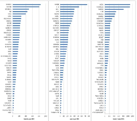
Figure 4.5: Graphs showing the distribution of the pediatric cases in the various counties for the three years of study

Figure 4.5 above shows distribution of cases for the different counties in the three years. We

observed that there is a high fluctuation in the incidence of pediatric TB during the three years of study. Of importance to observe was that counties like Mombasa, Nairobi, Kisii, Meru and

(41)

factors of overcrowding and urbanization. Counties like Lamu and Tharaka-nithi which have low

population were seen to record low cases.

4.1.2 Global Moran’s I

Being a composite index, the global Moran‟s index is the measure of overall clustering of the

data, used to evaluate the overall spatial association of the total research area. The Global Moran‟s uses the “z” statistic to evaluate the existence of clusters in the spatial arrangement of

the given data and shows the level of significance with the rule that if the “z” statistic value is greater than the value 1.96 then there is statistical significance. Also, while positive sign represents positive spatial autocorrelation, the converse is true for negative. The next three

Tables (Tables 4.1, 4.2 and 4.3) give a summary output of the results for the global Moran‟s index for the years 2009, 2010 and 2011.

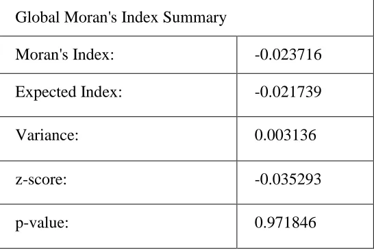
Table 4.1: Summary Table of the Global Moran’s Index output results for year 2009

Global Moran's Index Summary

Moran's Index: -0.023716

Expected Index: -0.021739

Variance: 0.003136

z-score: -0.035293

(42)

The results in Table 4.1 above gave the summary output for the global Moran‟s index for the

year 2009. We observed Global Moran‟s index to be 0.023716 with an expected value of -0.021739, a z-score of -0.035293 and a p-value of 0.971846. The Moran‟s index evaluated whether the pattern expressed is clustered, dispersed, or random. The index found to be

-0.023716 indicated a weak negative spatial autocorrelation in our data. Although our calculated index was close to zero, it is suggested tendency towards dispersion in pediatric TB cases for the

year 2009. This indicated a map pattern in which the geographic units (which are counties in our research) of similar values scattered throughout the map. The z-score of -0.035293 and a p-value of 0.971846 indicates statistical insignificance. This stated that feature values of the year 2009

were randomly distributed across the study area.

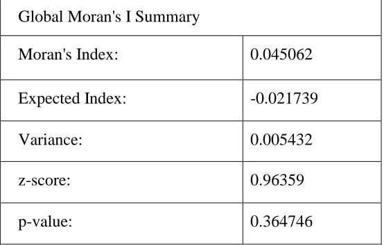
Table 4.2: Summary Table of the Global Moran’s I output results for year 2010

Global Moran's I Summary

Moran's Index: 0.045062

Variance: 0.005432

z-score: 0.96359

p-value: 0.364746

(43)

-0.045062 indicated a weak positive spatial autocorrelation in the data. The positive Moran's I

index value indicated tendency toward clustering in the pediatric cases for the year 2010. This

pointed out a map pattern in which the geographic units of similar values tend to cluster on the map. Also, the z-value found to be 0.96359 and p-value of 0.364746 like in 2009 depicted that

there is statistical insignificance. This stated that feature values again like in 2009 were also randomly distributed across the study area. Of importance to note was the magnitude for both the

Moran‟s index and also the p-value as they were in the increasing and decreasing trend respectively.

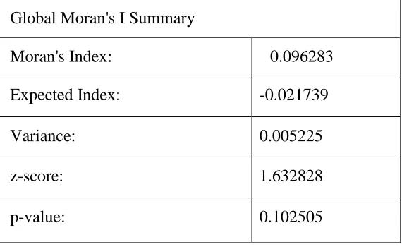
Table 4.3: Summary Table of the Global Moran’s I output results for year 2011

Global Moran's I Summary

Moran's Index: 0.096283

Variance: 0.005225

z-score: 1.632828

p-value: 0.102505

The results in Table 4.3 above presented summary output for the global Moran‟s index for year 2011. Moran‟s statistic was 0.096283 with an expected value of -0.021739, a z-score of

(44)

there was an increase in the Moran‟s index to 0.096283 and the positive spatial autocorrelation

indicated a map pattern in which the geographic units of similar values tend to cluster on the map.

Our findings for the global Moran‟s index were similar to the results by Peng et al. (2007) which

had a Moran‟s index of 0.1667 as both showed a pattern of spatial clustering. The z-score of 1.632828 and a p-value of 0.102505 still indicated that there was statistical insignificance in our

data for the year 2011. Of importance was that although there was statistical insignificance in our data, there was a drift towards statistical significance as indicated by the trend over the three

(45)

(a) (b)

(c)

(46)

Figure 4.6 above showed the incidence per 100,000 population. Figure 4.6 (a) showed the

distribution for the year 2009, Figure 4.6 (b) shows the distribution for the year 2010 while Figure 4.6 (c) shows the distribution of the cases for the year 2011. We observe generally that cases of pediatric tuberculosis are in all the counties rather, all counties have been affected and

that only the magnitude varies. For the year 2009, the incidence is high in the Rift valley south region and part of Nyanza and also some parts of Eastern and North Eastern as compared to

other regions in the country. Particularly, Nyamira, Kisii and Bomet recorded the highest incidence in the same year. This is shown in the Figure Figure 4.7 below. In the year 2010, the counties with high incidence of cases were Marsabit, Kitui, Westpokot, Embu and Siaya. In the

year 2011, the counties that were mostly affected were Kakamega, Vihiga, Kirinyaga and Meru. The other counties with high incidence were Marsabit, Isiolo, Samburu, Kilifi, Bomet, Mombasa

and Nairobi.

(47)

4.1.3 Local indicators of Spatial Association (LISA)

Local spatial statistics look for specific areas in an image that have clusters of similar or dissimilar values. The Local Moran‟s index identified counties clustering. Positive values for Local Moran‟s index indicates that a feature has neighbouring features with similarly high or low

attribute values; this feature is part of a cluster while negative values for Local Moran‟s index indicates that a feature has neighbouring features with dissimilar values; this feature is an outlier.

(48)

Figure 4.8 showed that some counties in the year 2009 had high-low relationship with its

neighbours. These were Samburu, Nyamira, part of Kisii and Bomet. It also showed the type of relationship that existed between the counties and its neighbours as high – low and not

significant.

Although showing that there was no statistical significant relationship for almost all the counties, Samburu and Nyamira both had a high – low type of relationship which indicated that the there

was a high reported incidence of pediatric TB cases in these two counties and surrounded by counties with low incidence of pediatric cases. This is an indication of clustering in these

counties.

Figure 4.9 below identified counties which had a statistically significant relationship with its neighbours. These included Kitui, Embu, Kirinyaga, Baringo, Uasingishu, Nandi, Kericho, Siaya

and Westpokot. It also showed the type of relationships where counties shaded red indicated a high – high relationship while counties shaded yellow indicated a high – low type of relationship

and that counties shaded blue indicated a low – low relationship.

For the findings of the three types of relationship, Baringo, Uasin-gishu, Nandi and Kericho counties all had a low – low type of relationship indicating that the counties had a low incidence

(49)

counties which had a high – high type of relationship meaning that these counties had a high

incidence of pediatric TB cases and the surrounding cases also had high incidence and hence implying clustering.

(50)

Figure 4.10: A map showing statistical significant relationship between counties and their neighbours in the year 2011

(51)

These were high –high and high – low. The counties observed to have a high- high relationship

with its neighbours were Isiolo, Meru and some part of Samburu. This type of relationship indicated that the respective counties had a high incidence of pediatric TB and surrounded by counties with high incidence. The other type of relationship which was of high – low indicated

that Kakamega and Vihiga had a high incidence and surrounded by counties with low incidence of pediatric tuberculosis. It was also observed that the type of relationship for a bigger part of our

study area was classified as insignificant.

4.1.4 Hot spot detection (Getis and Ord’s local statistic)

The Getis-Ord Gi index identifies hot spots. This is useful for determining clusters of similar values, where concentrations of high values result in a high Gi value and concentrations of low

values result in a low Gi value. The z-score values in Figures 4.11, 4.12 and 4.13 were used to identify the statistically significant counties. Specifically, a z-score value at 0.05 significance level would have to be less than -1.96 or greater than 1.96 to be statistically significant.

Statistical significance in the negative direction implies a cold spot while in the positive direction

implies hot spots. These Figures showed the behaviour of Getis and Ord‟s local statistic

(52)

Figure 4.11: A map showing the hot spot areas in the year 2009

Figure 4.11 above showed varying z-scores for the different counties. We observed that majority of the counties had z-score ranging between -1.65 to 1.65. Kiambu County had z-score value within the range of -1.96 and -1.65 while Migori County has z-score value within the range of

(53)

(statistically insignificant) while Kiambu and Migori depicted some tendency of dispersion and

clustering respectively.

(54)

Figure 4.12 above illustrated different z-score values for the year 2010. Majority of the counties

had z-scores ranging within -1.65 to 1.65. Counties like Mandera, Bungoma, Kakamega, Vihiga and Siaya had a z-score ranging from -1.96 to -1.65 while Baringo, Marakwet, Uasin-gishu, Nandi, Kisumu and Kericho had z-score within the range of -2.58 to -1.96. Kitui, Makueni,

Kajiado, Nairobi, Kiambu, Muranga, Embu, Meru and Kirinyaga had z-score values ranging within 1.96 to 2.58 and that Tharaka-Nithi and Machakos had z-score values greater than 2.58.

hence Machakos and Tharaka-Nithi were the hot spot counties while counties surrounding them indicated tendency towards being hot spots. Baringo, Marakwet, Uasin-gishu, Nandi, Kisumu

and Kericho showed tendency towards being cold spots.

The below map (Figure 4.13) showed different z-scores for the different counties in the year 2011. We observed that while majority of the counties had z-score values ranging from -1.65 to

1.65, Baringo county had a z-score within the range of -2.58 to -1.96. Marsabit had a z-score within the range of 1.65 to 1.96 while counties like Isiolo, Meru and part of Samburu had z-scores within the range of 1.96 to 2.58. There were no hot spots in the year 2011 but Isiolo and

(55)

Figure 4.13: A map showing the hot spot areas in the year 2011

4.1.5 Temporal analysis

(56)

the past to the present, or estimations of how spatial patterns will change from the present to the

future.

Table 4.4: A summary Table of the computed global Moran’s I for the years 2009, 2010 and 2011

Year Moran‟s I Expected (I) Variance (I) Z-Value P-Value 2009 -0.023716 -0.021739 0.003136 -0.035293 > -1.96 0.971846 2010 0.045062 -0.021739 0.005432 0.96359 < 1.96 0.364746 2011 0.096283 -0.021739 0.005225 1.632828 <1.96 0.102505

From the Table 4.4, we observed that the global Moran‟s I changed from -0.023716 for the year 2009 to 0.045062 for the year 2010 and then to 0.096283 for the year 2011 depicting an upward trend in the global statistic. The expected value (-0.021739) gave us the value of the Moran‟s I

when the pattern is random. When compared with the Moran‟s I, it was observed that there was an increasing trend in clustering of pediatric TB over the years of study.

Although using the three global maps produced for the years 2009, 2010 and 2011, we could not exactly visually discern whether or not spatial patterns were becoming concentrated or more dispersed, the computed Moran‟s I statistic for the three years depicted an increasing trend in the

value for Moran‟s I. It was evident therefore that there has been an overall clustering of the

(57)

In summary, the population of children under the age of 15 years (16571877) as indicated in our

methodology means that the number of children is 41430/100,000 population which forms 41.43% of the total population in Kenya. This is indeed a huge population and considering the age size, it can be classified as a vulnerable group in the sense that if infected, they are likely to

develop the disease. Also, if not treated they are likely to be the agents of future epidemic.

Although an exact picture of the incidence of childhood TB is difficult because of the difficulties

in the diagnosis of childhood TB, the incidence of 53/100,000 population for the year 2009, 42/100,000 population for the year 2010 and 56/100,000 population for the year 2011 from our results are a useful approximation of incidence. It is important to note that the cases could be

underestimated as some children would die undiagnosed.

Figure 4.6 hinted to us that the non-uniformity in the distribution of the pediatric cases in both

space and time for the different years of study allowing for further investigation. It was also observed that despite statistical non-significance in major parts of the country, the entire country has been reporting an increasing incidence of childhood TB and this if not prevented may result

in the disease being a future epidemic. Other than identifying counties with significant TB clusters for high rates of pediatric TB, we were also able to identify areas with suspected

elevation in risk. Spatial analysis showed hot spots of the disease.

(58)

different spatial distribution. Like the findings by Tong et al., (2009), Local Moran's I statistical

analysis could point out the high incidence region of childhood. Also, the findings of our study like that for Huang et al., (2010), showed that distribution of the incidence cases were not stochastic at space and time, and that clusters did exist. In consideration to LISA which is the

localized version of the global Moran‟s index, the findings portrayed that the incidence of pediatric TB varied for different counties. This gave some indication that the distribution of the

cases was not really random but rather, there was high concentration of cases in some parts while others had low concentration. This has been supported by the findings of Dirk et al. (2008) which indicated that the transmission of infectious diseases is closely linked to the concepts of spatial

and temporal proximity and hence transmission is more likely to occur if the at-risk individuals are close in a spatial and a temporal sense.

(59)

CHAPTER FIVE

SUMMARY, CONCLUSION AND

RECOMMENDATIONS

5.1 Introduction

This concluding Chapter summarizes the main findings, conclusions, recommendations and presents a brief discussion of possible areas for future research.

5.2 Summary

This research examined the dynamics of Tuberculosis disease in terms of both space and time at

the county level and obtained the pediatric map of Pediatric TB in Kenya. The global moran‟s statistic demonstrated an increasing trend towards clustering over the years of study. The LISA

statistic showed high-high relationships in some counties implying clustering. The G_i d

identified the hot spot counties. The spatial temporal distribution of the disease presented spatial –temporal patterns which provided an understanding of the disease dynamics and the high risk

areas where surveillance and control needed to be targeted.

5.3 Conclusion

First, the results showed some form of clustering which indicated that one county may be surrounded by other Counties with similar attributes implying that the closer a county is to another, the more similar the counties are. This confirms the Tobler‟s first law of geography

(60)

counties with hot spot areas in red and cold spots in blue which further indicated the existence of

sub-areas that developed pediatric TB differently over space.

Childhood TB is a sentinel of infectious adult prevalence and therefore childhood infection and disease rates need to be monitored in these high prevalence settings in order to ascertain the true

burden of infection and disease.

The spatial pattern of the disease has been seen to mirror the spatial pattern of the population at

risk which included the counties with high level of poverty and overcrowding. These identified areas of high risk will enable the Division of Leprosy, Tuberculosis and Lung Disease to propose innovative interventions to minimize the risk of disease at both individual and population level.

Also, it will help the Division in the effective deployment of resources. Keeping in mind the difficult in diagnosis of childhood TB, the cases reported might not be 100% efficient and hence

a need for tools to accurately and timely diagnose the presence of the disease or the infection and probably a mortality study be conducted to find out the causes of death among children.

Generally, this study has demonstrated the usefulness of spatial analysis in describing the geographical distribution of pediatric TB in the different counties in Kenya.

5.4 Recommendations

It will be very important for the Division of Leprosy Tuberculosis and Lung Disease to continue

(61)

The incidence of pediatric TB in this study was significant and that some counties were found to

be hot spots. Therefore, there is a need to have targeted intervention among these counties to ensure that Kenya strives to attain its fourth Millennium Development Goal (MDG) which is reduction in child mortality by preventing the loss of lives of innocent children through ways

which can be avoided.

Also because of the complexity in the diagnosis of tuberculosis in children, there is a probability

that the number of cases reported could be underestimated and hence there is need for refinement of existing tools and development and testing of new tools are urgently required to improve

diagnosis and treatment of TB in children.

Also, attention to childhood especially their nutrition and improvement in the socioeconomic and environmental condition in addition to reducing the burden of adult TB as stated by Rekha

(2010) is likely to have a significant impact on TB transmission to children.

We would also propose a sensitization of the DTLCs and health care workers at the facility so as to ensure a turnaround in the way we view tuberculosis in children and hence optimize reporting

of cases.

5.5 Areas for further research

It is possible to identify a number of areas for further research which will help to inform areas of policy interest. These include further studies on spatial distribution of tuberculosis in adults so as

(62)

associated with tuberculosis. Also, more studies need to be done on other infectious diseases e.g.

malaria so as to be able to identify the hot spots and their risk factors.

Further studies aimed at determining the hot spots areas of the infections among the general population will be of value in determining the population prevalence, so that proper public health

(63)

REFERENCES

Badri, M., Ehrlich, R., Wood, R., Pulerwitz, T., Maartens, G., (2001). Association between tuberculosis and HIV disease progression in a high tuberculosis prevalence area. Retrieve January 15, 2013, from www.ncbi.nlm.nih.gov: ttp://www.ncbi.nlm.nih.gov/pubmed/11326821.

Berke, O. (2004). Exploratory disease mapping: kriging the spatial risk function from regional count data. Retrieved from International Journal of Health Geographics: http://www.ij-healthgeographics.com/3/1/18.

Dirk, P., Timothy, P. R., Mark, S., Kim, B. S., David, J. R. and Archie, C. A. (2008).

Spatial Analysis in Epidemiology . United States: Oxford University Press Inc., New York.

DLTLD (2012). TB Control in Kenya. Retrieved January 17, 2012, from www.nltp.co.ke:

Huang, F., Cheng, S. M., Du, X., Chen, W., and Wang, L. X. (2010). Spatial analysis on new smear-positive pulmonary TB in China, 2003 - 2008. http://www.mendeley.com. [Online] 2010. [Cited: 02 07, 2012.] http://www.mendeley.com/research/spatial-analysis-new-smearpositive-pulmonary-TB-china-2003-2008/.

IRIN (2012). Stepping up paediatric TB diagnosis. (2012). Retrieved 02 09, 2012, from

http://www.plusnews.org:http://www.plusnews.org/Report/92277/KENYA-Stepping-up-paediatric-TB-diagnosis.

Ji-lei W., Wang J.,Zheng X. (2004). Spatial Exploratory Data Analysis of Birth Defect Risk Factors' Identification. http://en.cnki.com.cn. [Online] Chinese Academy ofScience,Beijing, 06 2004. [Cited: 02 07, 2012.] http://en.cnki.com.cn/Article_en/CJFDTOTAL- YJ200406003.htm.

(64)

Manoon, P. K.(2004). International Journal of Health Geographics. Retrieved from Using GIS technology to identify areas of tuberculosis transmission and incidence: http://www.ij-healthgeographics.com/content/3/1/23.

Middelkoop, K., Bekker, L., Carl, M., Zwane, E., and Robin, W. (2009). Childhood TB infection and disease: A spatial and temporal transmission analysis in a South African township. 738, 739.

Miller, H. J. (2004). Tobler‟s First Law and Spatial Analysis. Annals of the Association of American Geographers, pp 284-289.

Motsoaledi, A. (2011, April 19). How to Wipe Out TB. Retrieved February 10, 2012, from http://www.usnews.com: http://www.usnews.com/opinion/articles/2011/04/19/how-to-wipe-out-TB.

Peng, B., Zhang, Y., Daiyu, H. (2007). Using Spatial Analysis Technique To Explore Spatial Distribution Of TB. [Online] Chongqing Medical University,Chongqing, march 2007. [Cited: 02 07, 2012.] http://en.cnki.com.cn /Article_en/CJFDTOTAL-ZGWT200703001.htm.

Peter, D., Dermot, M., Shamim, Q. (2007). Improving the management of childhood tuberculosis within national tuberculosis programmes. A Research Agenda for Childhood tuberculosis, pp 3-4.

Phaisarn, J., Nitin, K. T., Marc, S. (2011). Spatio-Temporal Diffusion Pattern and Hot spot Detection of Dengue in Chachoengsao Province, Thailand. Environmental Research and Public Health .

Porter, J. (2002). Geographical information systems (GIS) and the TB DOTS strategy. http://onlinelibrary.wiley.com. [Online] A European journal TM & IH, January 5, 2002. [Cited: February 14, 2012.] http://onlinelibrary.wiley.com/doi/10.1046/j.1365-3156.1999.00475.x/full.

(65)

Rodrigues-Jr A., Ruffino-Netto A., Euclides A. (2006). Spatial distribution of M. TB/HIV coinfection in São Paulo State, Brazil,1991-2001.

Sandoz (2006). Sandoz. Retrieved January 30, 2012, from http://www.tbdots.com: http://www.tbdots.com/site/en/index.shtml.

Sartorius, B. (2011). Survived infancy but still vulnerable: spatial-temporal trends and risk factors for child mortality in the Agincourt rural sub-district, South Africa, 1992-2007. Geospatial Health.

Shi-ming C., Xin D., Min X. (2006). Surveillance and analysis of the pediatric pulmonary TB in new smear positive cases from 1992 to 2004 in China. http://www.mendeley.com. [Online] Chinese Journal Of Pediatrics, 2006. [Cited: 02 07, 2012.]

http://www.mendeley.com/research/surveillance-and-analysis-of-the-pediatric-pulmonary-TB-in-new-smear-positive-cases-from-1992-to-2004-in-china/.

Society (2012). Respiratory and Critical Care Medicine. Treatment of TB.

Tiwar, N. (2006). Investigation of geo-spatial hot spots for the occurrence of TB in Almora district, India, using GIS and spatial scan statistic. http://www.biomedcentral.com. [Online] International Journals of Geograhics, August 10, 2006. [Cited: February 14, 2012.] http://www.biomedcentral.com/1476-072X/5/33.

Tong, M., Zhang, H.,Sun, Y. (2009). The exploratory spatial data analysis of childhood TB in Mao county based on Geographic Information System. http://en.cnki.com.cn. [Online] the Chinese Center of Disease Prevention and Control,Beijing, 2009. [Cited: 02 07, 2012.] http://en.cnki.com.cn/Article_en/CJFDTOTAL-ZFYB200920017.htm.

(66)

Waller, L. A. (2006). Bayesian Thinking in Spatial Statistics. 1518 Clifton Road NE Atlanta, GA 30322.

Wikipedia (2012, Jan 17). www.wikipedia.org. [Online] Wikipedia, January 17, 2012. [Cited: January 19, 2012.] http://en.wikipedia.org/wiki/TB.

Wikipedia (2012, Jan 27). Wikipedia. Spatial analysis. http://en.wikipedia.org. [Online] January 27, 2012. [Cited: February 10, 2012.] http://en.wikipedia.org/wiki/Spatial_analysis.

(67)

APPENDICES

Appendix I : Data

COUNTY Cases _2009 popupation_ 2009 incidence-2009 Cases_ 2010 Population 2010 incidence 2010 Cases _2011 Population _ 2011 incidence 2011

BARINGO 51 269088 19 44 276850 16 53 284630 19

BOMET 48 187725 26 142 193140 74 211 198568 106

BUNGOMA 173 665255 26 225 684446 33 244 703679 35

BUSIA 187 356099 53 89 366371 24 157 376667 42

EMBU 165 193835 85 186 199427 93 93 205031 45

GARISSA 117 300952 39 28 309634 9 38 318335 12

HOMABAY 193 463485 42 247 476855 52 289 490255 59

ISIOLO 48 63558 76 43 65391 66 71 67229 106

KAJIADO 208 428390 49 225 440748 51 62 453133 14

KAKAMEGA 173 482530 36 195 496450 39 1087 510400 213

KEIYO-MARAKWET 138 171683 80 41 176636 23 8 181599 4

KERICHO 221 392579 56 76 403904 19 177 415254 43

KIAMBU 99 499731 20 365 514147 71 419 528595 79

KILIFI 167 518685 32 220 533647 41 488 548644 89

KIRINYAGA 68 175111 39 274 180162 152 232 185225 125

KISII 448 568580 79 235 584982 40 209 601421 35

KISUMU 226 421536 54 221 433696 51 218 445883 49

(68)

MARSABIT 74 136043 54 125 139967 89 182 143901 126

MERU 263 627856 42 400 645968 62 1104 664120 166

MIGORI 235 453768 52 305 466858 65 229 479977 48

MOMBASA 496 310117 160 332 319063 104 452 328029 138

MURANGA 93 412123 23 210 424011 50 172 435927 39

NAIROBI 810 951003 85 757 978437 77 814 1005932 81

NAKURU 120 670984 18 383 690340 55 142 709739 20

NANDI 131 338777 39 58 348550 17 23 358344 6

NAROK 109 286131 38 106 294385 36 228 302658 75

NYAMIRA 852 213793 399 80 219960 36 57 226141 25

NYANDARUA 56 256876 22 124 264286 47 98 271713 36

NYERI 38 234263 16 151 241021 63 147 247794 59

SAMBURU 224 113216 198 83 116482 71 127 119755 106

SIAYA 398 378343 105 389 389257 100 227 400196 57

TAITA-TAVETA 31 107209 29 73 110302 66 61 113401 54

TANA-RIVER 33 122099 27 32 125621 25 62 129151 48

THARAKA-NITHI 20 56819 35 25 58458 43 35 60101 58

TRANS-NZOIA 216 370635 58 88 381327 23 45 392042 11

TURKANA 249 393213 63 161 404556 40 78 415925 19

UASIN-GISHU 207 385102 54 42 396211 11 19 407345 5

VIHIGA 133 246971 54 28 254095 11 54 261236 21

WAJIR 89 278310 32 37 286338 13 47 294385 16