How to Make a Mudsparkler

(1)

University of South Carolina

Scholar Commons

Theses and Dissertations

2017

Functional Data Smoothing Methods and Their

Applications

Songqiao Huang

University of South Carolina

Follow this and additional works at:https://scholarcommons.sc.edu/etd

Part of theStatistics and Probability Commons

This Open Access Dissertation is brought to you by Scholar Commons. It has been accepted for inclusion in Theses and Dissertations by an authorized administrator of Scholar Commons. For more information, please [email protected].

Recommended Citation

Huang, S.(2017).Functional Data Smoothing Methods and Their Applications.(Doctoral dissertation). Retrieved from

(2)

Functional Data Smoothing Methods and Their Applications

by

Songqiao Huang

Bachelor of Science

Binghamton University, State University of New York, 2011

Submitted in Partial Fulfillment of the Requirements for the Degree of Doctor of Philosophy in

Statistics

College of Arts and Sciences University of South Carolina

2017 Accepted by:

David B. Hitchcock, Major Professor Paramita Chakraborty, Committee Member

Xiaoyan Lin, Committee Member Susan E. Steck, Committee Member

(3)

c

(4)

Dedication

(5)

Acknowledgments

I want to express my greatest gratitude to my academic advisor, Dr. David B. Hitch-cock, who has encouraged, inspired, motivated me, and guided me through all the obstacles in my Ph.D. study with great patience. Dr. Hitchcock is not only my aca-demic advisor, but is also a very good life mentor and friend. His knowledge, patience and carefulness toward research, and his great advice and encouragements for other aspects of life during my years at the University of South Carolina, Columbia have helped me grow and become stronger both academically and personally.

I also want to thank all of my committee members, Dr. Susan Steck, Dr. Paramita Chakraborty and Dr. Xiaoyan Lin for carefully reviewing my dissertation, and for their insightful suggestions and comments on my dissertation.

(6)

Abstract

(7)

(8)

List of Tables

Table 2.1 MSE comparison table for five smoothing methods. Top: MSE values calculated with respect to the observed curve. Bottom:

MSE values calculated with respect to the true signal curve. . . 37 Table 2.2 MSE comparison table for six smoothing methods. Digits in the

Weights column represent the weighting of the simulated peri-odic curve, smooth curve and spiky curve, respectively. Top row in each cell: MSE value calculated with respect to the observed curve. Bottom row in each cell: MSE value calculated with

re-spect to the true signal curve. . . 38

Table 3.1 Rand index values for five smoothing methods based on regular

distance matrix . . . 47 Table 3.2 Rand index values for five smoothing methods based on

stan-dardized distance matrix . . . 47 Table 3.3 In-sample SSE comparison for functional regression predictions

based on simulated curves . . . 50 Table 3.4 Out-of-sample SSE comparison for functional regression

predic-tions based on simulated curves . . . 55 Table 3.5 SSE comparison table: Model 1: both dew point and humidity

are predictors. Top: SSE for predicted response curves with re-spect to the true observed curve, no further smoothing onα1(t),

β11(t) and β12(t). Bottom: SSE for predicted response curves

with respect to the true signal curve, with further smoothing on

α1(t), β11(t) and β12(t) using regular B-spline basis functions. . . . 58 Table 3.6 In-sample SSE comparison: Model 2: dew point is the only

pre-dictor. Top: SSE for predicted response curves with respect to the true signal curve, no further smoothing on α2(t) and β1(t).

Bottom: SSE for predicted response curves with respect to the true observed curve, with further smoothing on α2(t) and β1(t)

(11)

Table 3.7 In-sample SSE comparison: Model 3: humidity is the only pre-dictor. Top: SSE for predicted response curves with respect to the true signal curve, no further smoothing on α3(t) and β2(t).

Bottom: SSE for predicted response curves with respect to the true observed curve, with further smoothing on α3(t) and β2(t)

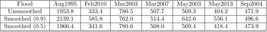
using regular B-splines basis functions. . . 61 Table 3.8 SSE comparison for seven flood events. Top: SSE values based

on functional regression without any smoothing. Bottom: SSE values based on functional regression with raw data curves and

estimated intercept and slope curves smoothed via smoothing splines. 68 Table 3.9 SSE comparison for seven flood events. SSE values based on

functional regression without any pre-smoothing on the obser-vation curves. “Cross-validation” idea is utilized to obtain out-of-sample predictions. Top: SSE values based on functional re-gression without any smoothing. Bottom: SSE values based on functional regression with raw data curves and estimated

inter-cept and slope curves smoothed via smoothing splines. . . 72 Table 3.10 SSE comparison for seven flood events. SSE values based on

functional regression with Bayesian transformed B-splines method

on the observed curves. . . 73 Table 3.11 SSE comparison for seven flood events. SSE values based on

functional regression with Bayesian transformed B-splines method on the observation curves. Top: No further smoothing on ˆα(t) and ˆβ(t) curves. Middle: ˆα(t) and ˆβ(t) curves further smoothed using smoothed splines with roughness parameter = 0.9. Bot-tom: ˆα(t) and ˆβ(t) curves further smoothed using smoothed

splines with roughness parameter = 0.5. . . 77 Table 3.12 SSE comparison for seven flood events. SSE values based on

functional regression with Bayesian transformed B-splines method on the observation curves. “Cross-validation” idea is utilized to obtain out-of-sample predictions. Top: No further smoothing on ˆα(t) and ˆβ(t) curves. Bottom: ˆα(t) and ˆβ(t) curves further

(12)

List of Figures

Figure 2.1 Comparison plot of two normal density curves. Dashed curve: density ofN(0, σ_di2 +c2_iζ_i2). Solid curve: density ofN(0, σ2_di+ζ_i2).

(ci, σdi/ζi) = (5,1). . . 20

Figure 2.2 Comparison plot of two normal density curves. Dashed curve: density ofN(0, σ2

di+c2iζi2). Solid curve: density ofN(0, σ2di+ζi2).

(ci, σdi/ζi) = (100,10). . . 20

Figure 2.3 True versus fitted simulated curves. Dashed spiky curve: sim-ulated true signal curve. Solid wiggly curve: corresponding

observed curve. . . 33 Figure 2.4 Mean squared error trace plot of 1000 MCMC iterations . . . 34 Figure 2.5 Example of set of 15 transformed B-splines obtained from one

MCMC iteration . . . 34 Figure 2.6 True signal curve versus fitted curves from three competing

methods. Black solid curve: true signal curve. Red dashed curve: fitted curve obtained from Bayesian transformed B-splines method. Blue dotted curve: fitted curve obtained from B-splines basis functions. Dashed green curve: fitted curve

ob-tained from B-splines basis functions with selected knots. . . 35 Figure 2.7 True signal curve versus fitted curves from three competing

methods. Black solid curve: true signal curve. Red dashed curve: fitted curve obtained from Bayesian transformed B-splines method. Blue dotted curve: fitted curve obtained from the wavelet basis functions. Dashed green curve: fitted curve

ob-tained from the Fourier basis functions. . . 36 Figure 2.8 Observed versus smoothed wind speed curves. Top: four

ob-served wind speed curves. Bottom: four corresponding wind speed curves smoothed with Bayesian transformed B-splines

(13)

Figure 2.9 Side by side boxplots of MSE values for five smoothing meth-ods. From left to right: boxplot of MSE values for 18 ocean wind curves smoothed with the selected knots B-splines (SKB); the B-splines with equally selected knots (B); the Wavelet basis (Wave); the Fourier basis (Fourier) and the Bayesian

trans-formed B-splines (TB). . . 40

Figure 3.1 Simulated curves from four clusters. . . 46 Figure 3.2 Boxplots of SSE values for the first 9 predicted response curves

with no presmoothing or presmoothing using the transformed splines, the Fourier basis, the Wavelet basis and regular B-splines basis functions on the curves. Red line: SSE value for the predicted response curves with presmoothing on the curves

using the transformed B-splines. . . 52 Figure 3.3 The first 9 predicted response curves. Black spiky curves: true

signal response curves. Red long dashed curves: predicted curves with presmoothing using the transformed B-splines. Pur-ple wiggly curves: predicted response curves with no presmooth-ing on the curves. Green dashed curve: predicted response

curves with presmoothing using the Fourier basis functions. . . . 53 Figure 3.4 The first 9 predicted response curves. Black spiky curves: true

signal response curves. Red long dashed curves: predicted curves with presmoothing using the transformed B-splines. Blue wiggly curves: predicted response curves with with presmooth-ing uspresmooth-ing the Wavelet basis functions. Green dashed curve: predicted response curves with presmoothing using the regular

B-spline basis functions. . . 54 Figure 3.5 True Orlando temperature curves and predicted response curves

without data smoothing, or with data presmoothed using the transformed B-spline basis and the Fourier basis functions. Black solid curve: true Orlando weather curves. Green solid curve: predicted curves without any data smoothing. Red solid curve: predicted curves with data presmoothed using the transformed B-spline basis functions. Purple dashed curve: predicted curves

(14)

Figure 3.6 True Orlando temperature curves and predicted response curves with data presmoothed using the transformed B-spline basis, regular B-spline basis functions and the wavelet basis func-tions. Black solid curve: true Orlando weather curves. Green solid curve: predicted curves presmoothed using the wavelet basis functions. Red solid curve: predicted curves with data presmoothed using the transformed B-spline basis functions. Purple dashed curve: predicted curves with data presmoothed

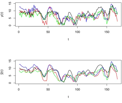
using regular B-spline basis functions. . . 60 Figure 3.7 Upstream (Congaree gage) water level measures for flood event

of October 2015. . . 62 Figure 3.8 Downstream (Cedar Creek gage) water level measures for flood

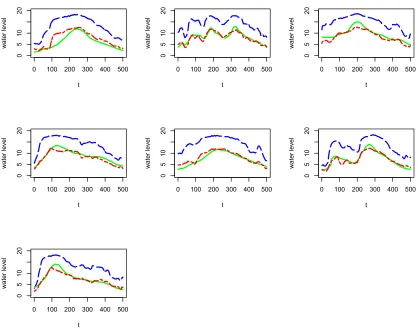
event of October 2015. . . 63 Figure 3.9 Downstream (Cedar Creek gage) and upstream (Congaree gage)

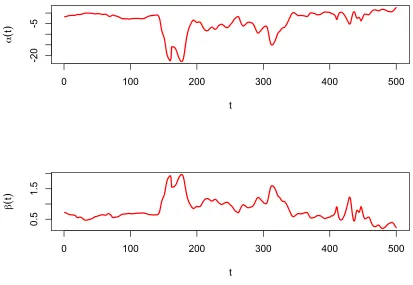
water level measures for six flood events. . . 64 Figure 3.10 Functional regression based on raw data curves. Top: intercept

function ˆα(t). Bottom: slope function ˆβ(t) . . . 66 Figure 3.11 Functional regression based on raw data curves. Blue dashed

curve: observed Congaree curve. Green solid curve: observed

Cedar Creek curve. Red dashed curve: predicted Cedar Creek curve. 67 Figure 3.12 Functional regression based on pre-smoothed data curves. Top:

smoothed intercept ˜α(t). Bottom: smoothed slope ˜β(t) . . . 68 Figure 3.13 Functional regression based on pre-smoothed data curves,

ob-tained intercept and slope curves are further smoothed for pre-diction. Blue dashed curve: smoothed Congaree curve. Green solid curve: smoothed Cedar Creek curve. Red dashed curve:

predicted Cedar Creek curve. . . 69 Figure 3.14 Functional regression based on pre-smoothed data curves,

ob-tained intercept and slope curves are further smoothed for pre-diction. Blue dashed curve: smoothed Congaree curve for Oc-tober 2015 event. Green solid curve: smoothed Cedar Creek curve for October 2015 event. Red dashed curve: predicted

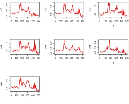
Cedar Creek curve for October 2015 event. . . 70 Figure 3.15 Obtained slopes for seven flood events using functional

(15)

Figure 3.16 Obtained slopes for seven flood events using functional regres-sion based on pre-smoothed data curves using “Cross-validation”

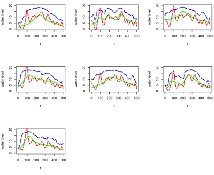
idea. . . 72 Figure 3.17 Functional regression based on pre-smoothed data curves using

Bayesian transformed B-splines method. Blue dashed curve: smoothed Congaree curve. Green solid curve: smoothed Cedar

Creek curve. Red dashed curve: predicted Cedar Creek curve. . . 74 Figure 3.18 Functional regression based on pre-smoothed data curves

us-ing Bayesian transformed B-splines method. Obtained ˆα(t) and ˆβ(t) curves are further smoothed using the same proce-dure. Blue dashed curve: smoothed Congaree curve. Green solid curve: smoothed Cedar Creek curve. Red dashed curve:

predicted Cedar Creek curve. . . 75 Figure 3.19 Functional regression based on pre-smoothed data curves

us-ing Bayesian transformed B-splines method. Obtained ˆα(t) and ˆβ(t) curves are further smoothed using smoothing splines with roughness penalty parameter = 0.9. Blue dashed curve: smoothed Congaree curve. Green solid curve: smoothed Cedar

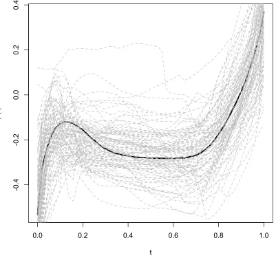
Creek curve. Red dashed curve: predicted Cedar Creek curve. . . 76 Figure 3.20 Estimatedα(t) andβ(t) curves smoothed using Bayesian

trans-formed B-splines method. Top: estimated (black) and smoothed (red) α(t) curve. Bottom: estimated (black) and smoothed

(red) β(t) curve. . . 78 Figure 3.21 Estimatedα(t) andβ(t) curves smoothed using smoothing splines

method with roughness penalty parameter = 0.9. Top: esti-mated (black) and smoothed (red) ˆα(t) curve. Bottom:

esti-mated (black) and smoothed (red) ˆβ(t) curve. . . 79 Figure 3.22 Functional regression based on pre-smoothed data curves using

the Bayesian transformed B-splines method. Obtained ˆα(t) and ˆ

β(t) curves are further smoothed using smoothing splines with roughness penalty parameters = 0.9 ( ˆα(t)) and 0.5 ( ˆβ(t)). Blue dashed curve: smoothed Congaree curve. Green solid curve: smoothed Cedar Creek curve. Red dashed curve: predicted

(16)

Figure 3.23 Estimatedα(t) andβ(t) curves smoothed using smoothing splines method with roughness penalty parameter = 0.9 ( ˆα(t)) and 0.5 ( ˆβ(t)). Top: estimated (black) and smoothed (red) α(t) curve.

Bottom: estimated (black) and smoothed (red) β(t) curve. . . 81 Figure 3.24 Functional regression based on pre-smoothed data curves using

the Bayesian transformed B-splines method. “Cross-validation” idea is utilized to obtain out-of-sample predictions. Blue dashed curve: smoothed Congaree curve. Green solid curve: smoothed

Cedar Creek curve. Red dashed curve: predicted Cedar Creek curve 83 Figure 3.25 Functional regression based on pre-smoothed data curves

us-ing the Bayesian transformed B-splines method. Obtained ˆα(t) and ˆβ(t) curves are further smoothed using smoothing splines method with roughness penalty parameter = 0.9. “Cross-validation” is utilized to obtain out-of-sample predictions. Blue dashed curve: smoothed Congaree curve. Green solid curve: smoothed

Cedar Creek curve. Red dashed curve: predicted Cedar Creek curve 84

Figure 4.1 Observed points versus smooth fitted curves. Left: colored curves: observed values for ten curves connected with linear interpolations for each curve. Right: colored curves: smooth fitted curves for all ten observations in the cluster; black dashed

curve: estimated common mean curve for the cluster. . . 107 Figure 4.2 Estimated common mean curve and mean trajectories from

multiple iterations. Black solid curve: estimated mean curve obtained from 1500 iterations after 500-iteration burn-in. Grey dashed curves: estimated common mean trajectories from 100

iterations. . . 108 Figure 4.3 95 percent credible intervals, the estimated curves, and the

esti-mated common mean curve for five observations. Orange dotted curves: pointwise 95 percent credible intervals for the curves. Red solid curves: median fits of the raw curves from the poste-rior distribution. Gray dashed curves: median of the estimated common mean curve obtained from the entire chain after a 500-iteration burn-in. Blue triangles: true observed values for the

(17)

Figure 4.4 95 percent credible intervals, the estimated curves, and the esti-mated common mean curve for five observations. Orange dotted curves: pointwise 95 percent credible intervals for the curves. Red solid curves: median fits of the raw curves from the poste-rior distribution. Gray dashed curves: median of the estimated common mean curve obtained from the entire chain after a 500-iteration burn-in. Blue triangles: true observed values for the

(18)

Chapter 1 Introduction

1.1 Literature Review

This section offers a brief literature review of functional data analysis (FDA) and some functional data applications. We start with a brief introduction of the origin of functional data analysis, and then discuss the development of the subject relating to our research.

Origin

(19)

perceiving continuous data curves. Instead of selecting a limited number of variables to represent the data, Ramsay and Dalzell viewed the curves themselves as individual observations, where each one is perceived as a function or mapping that takes values from a certain domain (usually a time interval) to some range that lies within the scope of interest for the response in the study, where the functions vary across the data set. Thus, the information about correlation across any time interval is contained in the function itself. In addition, it also enables the exploitation of information hid-den in higher-order derivatives of the original functional datum. Such information is often considered vital for understanding the behavior of the curves in practice. In sum, the main difference between classical multivariate analysis and FDA is that not only are the measured points perceived as variables on a continuous domain, but the functional itself is varying too (Ramsay 1982). On the other hand, similarly to classical multivariate data analysis, researchers can still analyze data by viewing a group of curves as a set of data. Straightforward statistical analysis of functional data include but are not limited to: classification and clustering, regression analysis, noise reduction and prediction.

Development

Over the last three decades, functional data analysis has been given more attention by researchers in biomedical fields. It has become common to analyze or interpret curves, or even images and their patterns from this new perspective. With the development of high-throughput technology, data can be measured over a very dense grid of points on a continuous domain, which makes functional data more prevalent.

(20)

For instance, Hitchcock, Casella and Booth (2006) proved that a shrinkage smoother effectively improves the accuracy of a dissimilarity measure between pairs of curves. Hitchcock, Booth and Casella (2007) showed that smoothing usually produces a more accurate clustering result, especially when a James-Stein-type shrinkage adjustment is applied to linear smoothers.

Popular data smoothing methods include basis fitting, regression splines, rough-ness penalty-related smooths, kernel-based smoothers, and smoothing splines. Among these categories, the regression spline is the most widely used method for data smooth-ing. The regression spline method refers to the functional data fitting approach employing basis functions called splines to form a “design matrix” as in classical re-gression. The fitted curve is obtained via the usual least squares (or weighted least squares) method, where the weight matrix usually involves the reciprocal of the cor-relation structure of the error terms. Knots sometimes split the domain into pieces in order to fit data piece by piece via usual regression methods. Hence determining the appropriate number and locations of the knots is a problem to be solved prior to or along with the data smoothing procedure. Polynomial splines and B-splines (de Boor 2001) are two examples that require selection of knots prior to data smooth-ing. Currently existing knot selection methods include Bayesian adaptive regression splines (BARS) (DiMatteo, Genovese and Kass 2001), which uses a Bayesian model to select an appropriate knot sequence using the data themselves. This approach employed the reversible jump Markov chain Monte Carlo (RJMCMC) Bayesian mod-eling scheme that is capable of determining the number of knots and their locations simultaneously (Green 1995). Another method with a similar aim is knot selection via penalized splines (Spiriti, Eubank, Smith and Young 2008). Other basis systems include but are not limited to the Fourier basis and the wavelet basis, for which least squares or weighted least squares fitting may also be employed.

(21)

must individually reflect the characteristics of the various functional observations. Currently there is no such unified basis system that can be applied automatically to a large collection of curves for accurate data fitting (Ramsay and Silverman 2005).

(22)

the smoothing spline framework, with the penalty term controlling the smoothness of the fitted curves. Methods like these are called penalized spline methods.

Then, however, the knot location problem returns. The most common solution is equal spacing of the knots (e.g., Ramsay and Silverman 2002), so that the only problem is to determine the number of knots to be placed on the domain. Obviously, such a method is only good for relatively simple structured curves with homogeneous behavior. For the general roughness penalty approach, the penalty term is not re-stricted to be the aforementioned derivative measure of the original curves; other forms of penalties such as the squared harmonic acceleration penalty may also be plausible.

Finally, the kernel-based fitting approaches are commonly used nonparametric data smoothing methods. The estimated curve evaluated at each individual point is still represented by a weighted average of the observed response values measured at different points on the domain. The main difference is that the weights are now determined by pre-specified kernel functions. The bandwidths of the kernels control the value of the weight at different points. Popular kernel functions include the uniform, the quadratic and variations of Gaussian kernels that are positive only over parts of the domain. This method falls into the category of localized least squares smoothing methods, since at each measured point, only some (not all) of the observed values are used for estimation of the curve. Nadaraya and Watson (Nadaraya 1964; Watson, 1964) proposed a way to standardize the specified kernel function, resulting in a unit sum weight function. Gasser and M¨uller (1979, 1984) further proposed a kernel-integral based weighting function that possesses good asymptotic properties and computational efficiency.

(23)

sparse functional data, see, e.g, Staniswalis and Lee (1998), Rice and Wu (2001), Yao, M¨uller and Wang (2005). Fitting methods based only on mixed effects models usually employ the EM algorithm to estimate important parameters of interest. However, as pointed out by James, Hastie and Sugar (2000), this approach could make the param-eter estimates highly variable when the data is very sparse. Hence, they proposed a reduced rank mixed effects model, which combines functional principal components with the mixed effects model by imposing several orthogonality constraints on the design matrices. An alternative approach incorporates the mixed effects models with the Bayesian technique, see Thompson and Rosen (2008) for details.

(24)

the other hand, was first introduced in Ramsay and Dalzell (1991), in which estima-tion of the parameter surface was obtained via a penalized least squares approach. A review of functional linear models can be found in Morris (2015). On the other hand, substantial studies of functional regression models have focused on the case of a scalar response and functional covariate. For this case, an easy approach is to smooth both the functional covariate and its corresponding coefficient with the same set of basis functions, say, B-splines, the Fourier basis or even smoothing splines (Cardot, Ferraty and Sarda 2003). By doing that, the smoothed functional linear model reduces to a classical linear regression. There are also numerous extensions of functional regression to functional generalized linear models. Both the cases in which the link function is known or is unknown have been substantially studied, e.g., (James 2002; Chen, Hall and M¨uller 2011). Functional regression has also been extended to the nonlinear case, where nonparametric smoothing is applied to functional predictors, see, e.g., Ferraty and Vieu (2006).

Another popular functional data application area that deals with groups of curves is functional cluster analysis. Similar to traditional cluster analysis, functional clus-tering typically involves traditional hierarchical, partitioning or model-based cluster-ing methods on the raw or standard distance matrices calculated based on the set of observed curves, the estimated basis function coefficients, or the principal component scores. See Abraham et al. (2003), James and Sugar (2003), Chiou and Li (2007) and Jacques and Preda (2014) for some studies in this area. A brief summary of current approaches for functional data clustering can be found at Wang et al. (2016).

1.2 Outline

(25)

intrinsically continuous, and data smoothing as a preliminary data analysis step has attracted considerable attention. It is reported in Ullah and Finch (2013) that more than 80 percent of functional data application papers under consideration utilized some kind of data smoothing prior to further analysis. However, data smoothing methods being considered still apply the classical ones to different types of observa-tions: regression splines, B-splines, smoothing splines, model-based methods, kernel-based approaches, etc. There is a lack of a more flexible method that could be adapted automatically to a broader range of curve forms. We therefore aim to fill this gap by proposing related methods that could be implemented more flexibly, and to examine subsequent impacts on other functional data inferences.

(26)

Chapter 2 Bayesian functional data fitting with

transformed B-splines

(27)

2.1 Introduction

Functional data analysis refers to the class of statistical analyses involving data that are collected on a set of points drawn from a continuum. The points at which data are collected are usually densely located over the continuum so that the curvature shape is captured properly. Functional data fitting then refers to some representation of the functional observations. Considering time-varying curves on 2-dimensional space, the model representation could refer to either: a linear combination of basis functions, fit, for example, via the least squares approach (e.g., de Boor 2001; Schumaker 2007); a linear combination of basis functions, augmented with terms consisting of a tuning parameter that controls the smoothness of the fitted curves and an integral of the functional outer products, such as the roughness penalty smoothing splines approach (de Boor 2001); or a moving average weighted by some kernel-based weight function, as in kernel smoothing of functional data.

(28)

squares approach or the roughness penalty approach, preliminary knowledge about the curves’ appearances is also essential to determine whether multiple knots should be placed at certain locations. When the data curve is intrinsically continuous yet changes rapidly in multiple locations, a B-spline basis might not be a wise choice. This is because multiple knots must be placed at several locations to depict those dramatic changes accurately, or else it may result in severe under-fitting. This would induce another potential issue: The total number of basis functions used to repre-sent the data may become undesirably large and the model may become much more complex than desired. In short, the accuracy of the model fit is achieved only by sac-rificing model simplicity. Triggered by these findings, we want to solve the following problems of interest simultaneously:

• To propose a method that would be appropriate for both well-behaved and irregular data curves.

• To improve data fitting with a fixed number of basis functions.

In the statistical literature on data smoothing, one notices that successful methods have been developed that construct new basis systems or adaptive splines to adjust for different shapes of the curves (e.g., Hastie, Tibshirani and Friedman 2009), yet there has been little focus on improving or transforming existing basis functions for greater flexibility. In this chapter, we propose a Bayesian fitting method that adjusts B-spline basis functions to accommodate data of a different nature. This approach avoids data inspection prior to smoothing and fits uniformly well for smooth, spiky, periodic or irregular data curves. To be more specific, we propose an “inverse-warping” transfor-mation on our pre-specified basis functions that lets the data determine the shape of the basis functions as well as their corresponding coefficients.

(29)

Bayesian model that generalizes the usage of basis functions to more than one shape of data curves. Section 2.4 describes the reversible jump Markov Chain Monte Carlo procedure we use in the simulations to optimally determine the number and locations of the knots that connect piecewise polynomials in B-splines for comparison purpose. Section 2.5 compares simulation results of our proposed method with four competing methods: B-splines with fixed knots; B-splines with optimally selected knots; the wavelet basis; and the Fourier basis. In section 2.6, we carry out our analysis on real data and compare our fitting results with other popular methods. Finally, section 2.7 includes some conclusion and discussion of our method.

2.2 Review of Concepts

B-splines

The popular B-spline basis function system was developed by de Boor (2001). These functions are a specific set of spline functions that share the property with regular splines of being piecewise polynomials connected via some knots on the time axis. The main difference is that there is a certain type of recursive relationship between B-spline basis functions of different orders, making it possible to derive higher-order functions once some lower-order basis functions are known. Furthermore, one can represent any spline function as a linear combination of these B-spline basis functions. We begin with assuming the following relationship between the data and the true signal:

y(ti) =x(ti) +i,∀i∈0, . . . , M −1

where ti is the ith time point, y(t) is the curve observed at t ∈T, hence y(ti) is the

observed value at timeti,x(ti) is the true underlying functionxevaluated at time ti,

(30)

functions φ evaluated at t:

x(t) =

nb

X

j=1

φj(t)cj,∀i∈0, . . . , M −1

where φj(t) is the jth basis function evaluated at time t, cj is the coefficient cor-responding to the jth basis function, and nb is the total number of basis functions

used. To obtain an estimate for x(t), one only needs to determine the basis func-tions and then estimate the coefficient valuescj via either the least squares approach,

weighted least squares approach, roughness penalty approach, etc. In particular, the

φj(t)’s in the B-spline basis system are piecewise spline functions of orderr, connected

smoothly at the time points where the knots are located, and defined over the entire region fromt0 totM−1. Denote the kth order piecewise spline in the interval [ti, ti+1)

asBi,k. Then the B-spline basis functions are constructed as follows:

Bi,0(t) =

    

   

1, if ti ≤t < ti+1.

0, otherwise.

and

Bi,k(t) =

t−ti ti+k−1 −ti

Bi,k−1(t) +

ti+k−t ti+k−ti+1

Bi+1,k−1(t)

As we can see from the recursive relationship above, each basis function evalu-ated at time t, Bi,k(t), could be obtained given the knowledge of the values of its

“neighbors”, Bi,k−1(t) and Bi+1,k−1(t). With such a construction method defined,

each φj(·) is restricted to be positive only on the minimal number of subintervals

divided by the knots. To be more specific, B-spline basis functions have the so-called

compact support property, which means that each φj(·) can be positive only over no more than k subintervals. This property guarantees the computational speed of the fitting algorithm to be O(nb) due to the M ×nb band-structured model

ma-trix Φ(t) (having entries being the B-spline functions evaluated at different time points t= (t0, t1, . . . , tM−1)0) no matter how many knots are included in the interval

(31)

One may determine the order of the spline functions based on the number of derivatives of the original curves that we require to be smooth. In practice, order-four polynomials are usually adequate to fit curves that are intrinsically smooth. Note that the placement of the knots on the time axis plays a vital role in the fitting performance of B-spline basis. If the number of knots is too small, the B-spline basis does not gain much flexibility in fitting curves beyond what a polynomial basis would have. However, increasingnb via using a greater number of knots might not always enhance the fit of the B-spline approximation to the data. In fact, Ramsay and Silverman (2005) imply that an improved fit would be achieved when nb is increased only by

adding a new knot to the existing sequence of knots, or by increasing the order of the spline functions while leaving the positions of the knots unchanged. Knots that are poorly located may influence the fit badly by emphasizing mild curvatures too much, and neglecting local areas that change rapidly in the curves. Ramsay and Silverman (2005) suggest that one may locate an equally spaced sequence of knots on the time axis if the data points are roughly balanced over the interval (t0, tM−1). However, if

(32)

Time Warping for Data Registration

The traditional use of a warping function is to transform the time axis in order to align a group of functional curves. Typically such curves are measured at the same time points, yet important landmarks may occur at different positions in chronological time. In order to subsequently carry out cluster analysis or some other type of statistical analysis, one may determine g landmark time points {t∗₁, t∗₂, . . . , t∗_g} that are viewed as standard times when certain events occur. Then the time axis for each individual observation is distorted so that the occurrence times of those landmark events are standardized. In other words, for the sth individual among a total of S

member curves, a time transformation Ws is imposed. Assume that the time points

at which those landmark events occur for curve s are {ts₁, ts₂, . . . , ts_g}. Then we have

Ws(·) that satisfies:

Ws(t0) =t0, Ws(tM−1) = tM−1,∀s,

and

Ws(tsi) =t ∗

i,∀i,∀s.

Also,Ws is a monotonic transformation that maintains the order of the transformed

time sequence. These Ws functions are called time-warping functions. Applying the

warping functions to the measured time points produces the warpedsth curve:

x∗_s(t) = xs(Ws(t)),∀t∈T

which has the same occurrence times for those landmarked events as does the standard time sequence. Given such properties of the warping functions, we can then obtain their inverse functionsW−1

s (t) by simple interpolation withW −1

s (t) on the horizontal

(33)

2.3 Bayesian Model Fitting for Functional Curves

Motivated by the idea of time warping to register curves, in order to improve the performance of curve fitting based on the set of pre-specified basis functions, we impose some transformation of the time axis for each of the basis functions to obtain a set of “inversely-warped” basis functions. This is done not to align the basis functions, but to provide some flexibility for them to improve the ultimate fit to the functional data. The transformation function, which is denoted as W(·), has to be monotone to preserve the order of the transformed time points. We will employ ideas from the Bayesian method of Cheng, Dryden and Huang (2016) to obtain the warping functions.

Assume that all the functional data are standardized so that their domains are [0,1] prior to carrying out further analysis. We use the notation t= {t0, t1, t2, . . . , tM−1}

to denote the parameterized time span; thus t0 = 0 < t1 < · · · < tM−1 = 1. Then

the transformation function W(·) or warping from the original time sequence t to a mapped new time sequence tw could be obtained as follows: first we generate

a sequence of M −1 numbers p = {p1, p2, . . . , pM−1} between 0 and 1, such that

PM−1

i=1 pi = 1. Then calculate the cumulative sum of the generated sequence p, we

obtain{p1, p1+p2, . . . , p1+p2+. . .+pM−2,1}which is a monotone sequence fromp1to

1. Finally, we define W(·) to be the mappingW(t) ={0, p1, p1+p2, . . . ,PMi=1−2pi,1}.

Following Cheng et al. (2016), to model the prior distribution of such a trans-formation on time, we view {0, p1, p1+p2, . . . , p1+p2 +. . .+pM−2,1}as a stepwise

cumulative distribution function (CDF) in the sense that the height of theith “jump” in the CDF graph corresponds to the value of pi in p. Therefore we could use the

Dirichlet distribution as the prior distribution to model the heights of all M −1 “jumps” in the step function. That is:

(34)

wherea= (a1, a2, . . . , aM−1)0 is the vector of hyperparameters in the Dirichlet

distri-bution that controls the amount of warping of the time points. Great discrepancies in the a values lead to significantly different means for the heights of the jumps in the cdf. When all the elements in a are equal, the elements’ magnitude controls the deviation of the transformed time points from the original time points. Smaller values ina correspond to greater deviation between the original time span and the warped time span. Therefore, a serves as a tuning parameter that influences the amount of warping of the time axis. In practice, due to computational concerns, one may choose to generate Mt≤M “jumps” via the Dirichlet distribution. One could label

tw ={tw0, tw1, . . . , tw_Mt−1}={0, p1, p1+p2, . . . , p1+p2+. . .+pMt−2,1}.

If Mt =M, one could define a different mapping Wj : t 7→ twj for the jth basis

functions as described above. LetΦ(t) be theM×nb matrix with the columns being

a set of nb pre-determined basis functions evaluated at t, and Φ∗(t) be a matrix of

the same dimensions with the columns being the set of nb “inversely warped” basis functions measured att. Note that we “inversely warp” each basis function differently, hence from now on, we use W, TW and P to denote the “vector of mappings”, the

“vector of transformed time sequences” and the “vector of increment vectors” for all basis functions, i.e., W = {W1, W2, . . . , Wnb}, TW = {tw1,tw2, . . . ,tw_nb} and P = {p1, . . . ,pnb}. To obtain Φ∗(t) once Φ(t) is given, we assume the following

relationship:

Φ(t) = Φ∗(W(t)) =Φ∗(TW).

Then if we regard Φ(·) and Φ∗(·) as functions that are applied on the same time vector t, we have Φ=Φ∗◦W. In what follows, we have:

Φ∗(t) =Φ∗(W−1(TW)) =Φ∗(W−1(W(t))) =Φ∗(W(W−1(t))) =Φ(W−1(t)).

(35)

Wj(t) on the x-axis andton the y-axis, then doing linear interpolation to obtain the

estimated values of the curve at vectort. Hence, Φ∗(t) can be estimated.

In the case that Mt< M, one could define a new time vector tnew with a smaller

length Mt that mimics the behavior of t. One could then apply the transformation

described above to obtainΦ∗(tnew), and approximate the M×nb dimensional matrix Φ∗(t) based on Φ∗(tnew).

Now we are able to give the model for the data. We start with functional data

y(t), wheretis the aforementioned standardized time vector. We assume a parametric model for our data:

y(t)|Φ(t),P, σ2 ∼M V N(Φ(W−1(t))d, σ2I),

where d is the vector of coefficients corresponding to those “inversely-warped” basis functions, and σ2 _{is the variance of the error terms.}

It is well known that the B-spline basis system is a powerful tool to fit a variety of types of curves. One can always achieve greater flexibility in data fitting by adding more knots on the time axis when the order of the basis functions is fixed, or by increasing the order of the basis functions while the number and the locations of the knots are fixed. Either approach requires an increase in the total number of basis functions to achieve better accuracy. But models that are overly complicated are not always desirable. We want to reduce the dimensionality of our model without sacrificing much accuracy, when our model dimensionality is not small. Hence we use an optional add-on indicator vectorγ ={γ1, γ2, . . . , γnb} in our procedure, such that

each of the γi follows a Bernoulli distribution with success probabilityαi, andγi = 1 denotes the presence of variable i. To incorporate this variable selection indicator

(36)

McCulloch (1993). O’Hara and Sillanpaa (2009) compared different Bayesian variable selection methods with respect to their program running speed, ability to jump back and forth between different stochastic stages and effectiveness of distinguishing truly significant variables from redundant variables. Based on the discussion of O’Hara and Sillanpaa (2009), we adopt the conditional prior structure ford|γand σ2_|_γ _described

in the stochastic search variable selection of George and McCulloch (1993), due to its relatively fast program running speed, ease ofγ jumping from stage to stage, and great power of separating important variables from trivial ones. The model is as follows:

d|γ ∼M V Nnb(0nb×1,DγRDγ),

σ2|γ ∼IG(νγ/2, νγλγ/2).

Here R can be viewed as the correlation matrix of d|γ; Therefore, George and Mc-Culloch (1993) suggest choosingR based on one’s prior knowledge of the correlations between each pair of coefficients given the information in γ. Dγ is a diagonal matrix

that determines the scale of variances of different coefficients. The model information for each MCMC iteration is stored in Dγ. In other words, the (i, i) element in Dγ

equalssiζi, whereζiis some fixed value and is usually determined by some data-driven method prior to the MCMC iterations. On the other hand, si depends on model

in-formation via some pre-specified value ci in the following way: si = c I(γi=1)

i . To be

more specific, the marginal distribution of di|γi is given by the following mixture of

normal distributions:

di|γi ∼(1−γi)N(0, ζi2) +γiN(0, c2iζi2).

Notice that eachdi, givenγi, follows eitherN(0, ζ_i2) orN(0, c2_iζ_i2). Then the estimate ˆ

di ofdi givenγi, followsN(0, σ2di+c2iζi2) forγi = 1 andN(0, σdi2 +ζi2) forγi = 0. Here

the σ2

(37)

Figure 2.1: Comparison plot of two normal density curves. Dashed curve: density of

N(0, σ_di2 +c2_iζ_i2). Solid curve: density ofN(0, σ_di2 +ζ_i2). (ci, σdi/ζi) = (5,1).

Figure 2.2: Comparison plot of two normal density curves. Dashed curve: density of

N(0, σ_di2 +c2_iζ_i2). Solid curve: density ofN(0, σ_di2 +ζ_i2). (ci, σdi/ζi) = (100,10).

functions superimposed on another shows, for each iteration, how the probability of including the ith basis function changes with different values of di.

Via observation of the separation of the two density curves, one also gets an idea of whether the prior ofdi|γi favors a parsimonious model or a more saturated model.

(38)

in the model is given by: γi = v u u t σ2

di/ζi2+c2i σ2

di/ζi2+ 1 .

Notice that the formula above depends only onσ2

di/ζi2andc2i, and as a result, one may

treat the combination of σ2

di/ζi2 and c2i as tuning parameters that determine model

complexity. Therefore, the values ofci andζi to be adopted in the simulations can be

determined by choosing different combinations of ˆσdi/ζiandcias needed, where ˆσdi/ζi

is the estimated variance of di. Figures 2.1 and 2.2 are two examples of such density curves superimposed on another, with (ci, σdi/ζi) chosen to be (5,1) and (100,10).

The νγ and λγ that appear in the inverse gamma prior of σ2|γ can depend on γ via the size of γ. When νγ is set to be zero, it reduces to the improper prior

σ2_|_γ_∼₁_/σ2_.

Lastly, since the measurement errors induced in the data collection process could be correlated in a systematic way instead of being independent across all time points, we also consider the possibility of using a more general correlation matrixCto model the association among the error terms. We will specifically consider the case when the error terms are correlated according to a AR(1) model. That is:

y(t)|Φ(t),P, σ2 ∼M V N(Φ(W−1(t))d, σ2C),

where C=                

1 ρ ρ2 · · · ρ(M−1) ρ 1 ρ · · · ρ(M−2)

..

. 1 · · ·

. ..

ρ(M−1) _{· · ·} _ρ ₁

                .

In this case, we will need a prior forρ. We propose to use:

(39)

to declare ignorance of the structure of the correlation between adjacent error terms. Assuming that P, σ2_{, ρ,}_d _{are independent given} _γ_{, and then we are able to derive}

the posterior distribution when the error terms are correlated according to a AR(1) model:

π(P,d, σ2, ρ,γ|y(t)) = f(P, σ

2_{, ρ,}_d_,_γ_{, y}₍_t₎₎ f(y(t))

∝f(y(t)|P, σ2, ρ,d,γ)·f(P, σ2, ρ,d|γ)·f(γ)

=f(y(t)|P, σ2, ρ,d,γ)·f(P)·f(σ2|γ)·f(ρ)·f(d|γ)·P(γ)

∝(det(σ2C))−0.5σ−νγ−2_exp (

−νγλγ

2σ2

)

×exp{−0.5d0(DγRDγ)−1d}I{−1≤ρ≤1}

×exp{−0.5(y(t)−Φ(W−1(t))d)0L0L(y(t)−Φ(W−1(t))d)} ×(det(DγRDγ))−0.5

nb

Y

k=1 M−1

Y

i=1

p(aik_ik −1) nb

Y

j=1

αγj_j (1−αj)(1−γj).

Here

L= 1

σq(1−ρ2₎

                q

(1−ρ2₎ ₀ ₀ _{· · ·} ₀ ₀

−ρ 1 0 · · · 0 0 0 −ρ 1 0 · · · 0

..

. . .. ...

0 · · · −ρ 1

                ,

where L0L is the Cholesky decomposition of _σ12C

−1_{(Jones 2011),} _p

ik denotes the

height of theith “jump” in the time span of the kth basis function pk,aik is the ith

parameter in the vector aof the Dirichlet distribution for the kth basis function, and

αj is the probability that the jth basis function is truly important (so that γj = 1)

in the model. Note that we use the subscript k to emphasize the fact that a could vary across basis functions.

We also must rewrite det(C). Letting L∗ =σL, then:

(40)

After some matrix manipulations and mathematical induction, we obtain:

L∗−1 =

               

1 0 · · · 0

ρ √1−ρ2 ₀ _{· · ·} ₀ ρ2 ρ√1−ρ2 √₁₋_ρ2 _{· · ·} ₀

..

. . .. . ..

ρM−1 _{· · ·} _ρ√₁₋_ρ2 √₁₋_ρ2

                ,

Therefore, the full posterior distribution is:

π(P,d, σ2, ρ,γ|y(t))∝σ−M−νγ−2_exp (

−νγλγ

2σ2

)

exp{−0.5d0(DγRDγ)−1d}

×exp{−0.5(y(t)−Φ(W−1(t))d)0L0L(y(t)−Φ(W−1(t))d)} ×(1−ρ2)−0.5(M−1)I{−1≤ρ≤1}(det(DγRDγ))−0.5

×

nb

Y

k=1 M−1

Y

i=1

p(aik−1) ik

nb

Y

j=1

αγj_j (1−αj)(1−γj).

Note that when one assumes that there is no apparent autocorrelation relationship in the error terms,L is replaced by the identity matrix, and ρ by 0 in the expression above. Then the posterior distribution of the jth element of γ, given the other information, could be obtained from:

f(γj|y(t),P, σ2, ρ,d,γ(j)) = f(γj|σ2,d,γ(j))

where γ_(j) denotes the current vector of γ, excluding the jth element. It is obvious that the posterior distribution of (γj|other information) is still a Bernoulli

distribu-tion, and the probability of success is given by:

P(γj = 1|σ2,d,γ(j)) =

f(σ2_|_γ

j = 1,γ(j))f(d|γj = 1,γ(j))P(γj = 1,γ(j)) f(σ2_,_d_,_γ

(j))

= u

u+v,

and similarly, the probability of failure is:

P(γj = 0|σ2,d,γ(j)) =

f(σ2_|_γ

j = 0,γ(j))f(d|γj = 0,γ(j))P(γj = 0,γ(j)) f(σ2_,_d_,_γ

(j))

= v

u+v,

(41)

The conditional posterior distribution of (d|other parameters) is given by:

f(d|y(t), ρ, σ2,γ)

∝exp{−0.5(y(t)−Φ(W−1(t))d)0L0L(y(t)−Φ(W−1(t))d)} ×exp{−0.5d0(DγRDγ)−1d}

∝exp

(

−0.5d0{Φ(W−1(t))0L0LΦ(W−1(t)) + (DγRDγ)−1}d −2y(t)0L0LΦ(W−1(t))

)

.

It is obvious that:

d|y(t),p, σ2, ρ,γ ∼M V N(µ_F,Σ),

where

µ_F =Σ[Φ(W−1(t))0L0Ly(t)],

and

Σ= [Φ(W−1(t))L0LΦ(W−1(t)) + (DγRDγ)−1]−1.

The posterior conditional distribution of σ2 is:

f(σ2|y(t),P, ρ,d,γ) =f(σ2|y(t), ρ,d,γ)

∝σ−M−νγ−2_exp (

− 1

2σ2 νγλγ + (y(t)−Φ(W

−1₍_t₎₎_d₎0

×L∗0L∗(y(t)−Φ(W−1(t))d)

!)

.

Thus,

σ2|y(t),P, ρ,d,γ ∼IG(α∗, β∗),

where

α∗ = M +νγ 2 , and

β∗ = 1

2 νγλγ + (y(t)−Φ(W

−1₍_t₎₎_d₎0_L∗0_L∗₍_y₍_t₎₋_Φ₍_W−1₍_t₎₎_d₎

!

(42)

Note that the information about basis function selection is contained in the posterior distribution ofγ. We employ the posterior mode of γ as defining the most desirable potential model, as described in George and McCulloch (1993). That is, we sample from the joint posterior distribution in the following order: p1,p2, . . . ,pnb, σ2,d,γ,p1, p2, . . . ,pnb, σ2, . . . . We utilize the Gibbs sampler to sample γ, σ2 and d, since their

conditional posterior distributions are known and easy to sample from, and we use Metropolis-Hastings method within the Gibbs sampler to samplePand ρ, since their conditional posterior distributions are not in closed form. Due to the restrictions on eachpk vector, we use a truncated normal distribution as the instrumental

distribu-tion. Let superscript (i) represents parameter values sampled at the ith iteration. For thekth basis function, one first generates an initial p(0)_k = (p(0)_1k, p(0)_2k, . . . , p(0)_Mt₋_1k)0 from a Dirichlet prior. Then at iteration i, one samples the elements of p(i)_k one by one in the following way:

1. Sample the first element in p(i)_k , p(i)_1k, by drawing a random observation from

N(p(i_1k−1), σ2₂)I(0, L_u1). And then adjust the last element inp(i_k−1), i.e.,p(i_Mt−₋1)_1k, to make the following holds:

p(i)_1k +

Mt−2

X

j=2

p(i_jk−1)+p(i_Mt−₋1)_1k= 1.

Denote the adjustedp(i_Mt−₋1)_1k asp∗_Mt(i)₋_1k. HereL1 u =p

(i−1)

1k +p

(i−1)

Mt−1k. If the proposedp (i) 1k,

denoted asp∗_1k(i), is accepted by the Metropolis-Hastings algorithm, then the first and the last elements in p(i)_k are updated as p_1k∗(i) and p∗_Mt(i)₋_1k, respectively, other elements are the same as those inp(i−1)_{. Otherwise, the entire vector} _p(i)

k remains the same as p(i_k−1).

2. For j = 2,3, . . . ,(Mt−2), sample the jth element p (i)

jk by drawing a random

observation fromN(p(i_jk−1), σ2

2)I(0, Lju), and adjustp ∗(i)

Mt−1k to make the following holds: Mt−2

X

j=1

p(i)_jk +p∗_Mt(i)₋_1k = 1.

Still denote the adjustedp∗_Mt(i)₋_1kasp∗_Mt(i)₋_1k. HereLj u =p

(i−1)

jk +p

∗(i)

(43)

p(i)_jk, denoted asp∗_jk(i), is accepted by the Metropolis-Hastings algorithm, then the jth and the last elements in p(i)_k are updated as p_jk∗(i) and p∗_Mt(i)₋_1k, respectively, other elements are kept unchanged. Otherwise, the entire vector p(i)_k remains unchanged.

Note that for any arbitrary iterationi, each time we sample, say, thejth element, the upper bound of the truncated normal distribution is adjusted based on the fact that it has to be less than p(i_jk−1) +p(i_Mt−₋1)_1k or p(i_jk−1) +p∗_Mt(i)₋_1k, in order to obtain a non-negative adjusted p(i)_Mt₋_1k in the vector.

For iteration i, with the proposedpjk inp (i)

k denoted as p ∗(i)

jk , the acceptance ratio

is given by:

a(p∗_jk(i), p(i_jk−1)) = π(p

∗(i) jk ) π(p(i_jk−1))

q(p(i_jk−1)|p∗_jk(i))

q(p∗_jk(i)|p(i_jk−1)),

where q(·|·) represents the truncated normal distribution N(·, σ₂2)I(0, Lj_u). Hence:

q(p(i_jk−1)|p∗_jki)

q(p∗i jk|p

(i−1)

jk )

= Φ(

Lju−p (i−1) jk

σ2 )−Φ(

−p(i−1)_jk

σ2 )

Φ(L

j u−p

∗(i) jk

σ2 )−Φ(

−p∗(i)_jk

σ2 ) .

Here Φ denotes the cumulative distribution function of the standard normal distri-bution. Then it follows that:

log(a(p∗_jk(i), p(i_jk−1))) =

log(π(p∗_jk(i))) + log



Φ

Lj u−p

(i−1) jk σ2

!

−Φ −p

(i−1) jk σ2 !  − 

log(π(p

(i−1)

jk )) + log Φ Lj

u−p ∗(i) jk σ2

!

−Φ −p

∗(i) jk σ2

!!



=−0.5(y(t)−Φ∗(i)(W−1(t))d)0L0L(y(t)−Φ∗(i)(W−1(t))d) +

nb

X

r=1 M−1

X

i=1

log(p∗_ir(i)(air−1)) + log



Φ

Lj u−p

(i−1) jk σ2

!

−Φ −p

(i−1) jk σ2

!



+ 0.5(y(t)−Φ(i−1)(W−1(t))d)0L0L(y(t)−Φ(i−1)(W−1(t))d)

−

nb

X

r=1 M−1

X

i=1

log(p(i_ir−1)(air−1))−log



Φ

Lj_u−p∗_jk(i) σ2

!

−Φ −p

∗(i) jk σ2

!

(44)

whereΦ∗(i)₍_W−1₍_t_{)) represents the adjusted “design matrix” in the}_i_{th step according}

top∗_jk(i).

2.4 Knot Selection with Reversible Jump MCMC

The flexibility of B-splines for fitting functional data is based on the knots on the time axis. Appropriately chosen knots could result in an extremely good fit, while naively chosen knots that do not reflect the nature of the functional curve could produce a poorly fitted curve. Hence, we will consider both cases of fixed knots and optimally selected knots in the simulation section.

Many methods have been developed that focus on selecting knots to improve the performance of B-splines. We will discuss two approaches proposed by Denison et al. (1998) and DiMatteo et al. (2001) that utilize Reversible Jump Markov Chain Monte Carlo (RJMCMC) (Green 1995) to simulate the posterior distribution of (k,ξ), where

(45)

the dimension of the parameters by having an additional proposed knot inserted into the existing knot sequence, accepts having one of the knots deleted from the sequence, or rejects the proposed state and stays at the current state. In the “relocation step,” the chain determines whether to relocate one of the existing knots or not.

Because the underlying true model is not unique, we assume that with appropri-ately chosen knots, the observed data could be adequappropri-ately described with a group of order r B-splines. The data and the “design matrix” formed by the B-splines evaluated at those measured time points are connected via the following relationship:

y(t)|Φk,ξ(t), σ2B∼M V Nr+k(Φk,ξ(t)c, σB2I),

where c is the true underlying vector of coefficients corresponding to the B-splines in the model, and σ2

B is the variance of the error terms. Here the subscripts in the

notationΦk,ξ(t) are used to emphasize how both the dimension and the values of the

B-spline functions depend on the number and locations of the knots. Note that while independent errors are assumed here, one may certainly include some autocorrelation structure to allow for the possibility of correlated error terms. However, in a two-stage procedure, where one first selects knots on the time axis for optimal B-splines performance, and then uses our Bayesian model described in section 2.3 to further improve the fit, the structure of error terms for both stages should coincide with each other. We use the scheme given by DiMatteo et al. (2001). The prior for k is Poisson, and ξ|k follows Dir(1,1,. . . , 1). The prior for σ_B2 could be chosen as inverse gamma or the improper priorπ(σ_B2)∼1/σ2_B. The coefficient vector has the following conditional prior:

c|k,ξ, σ2_B ∼M V N(0, σ_B2M{Φk,ξ(t)TΦk,ξ(t)}−1).

In each iteration, the three aforementioned probabilities are given by:

(46)

where bk is the probability of jumping from k interior knots to k+ 1 interior knots.

Whether the chain at the next iteration moves to the state with an additional interior knot depends on the acceptance ratio. Similarly,ekis the probability of jumping from k interior knots to the state with k−1 interior knots. Such a move may or may not be made based on the acceptance ratio. hk is the probability of relocating one of the

existing knots.

The main discrepancy between Denison et al. (1998) and DiMatteo et al. (2001) is that the first utilizes a not entirely Bayesian approach, but rather a quasi-Bayesian approach to generate the chain by using least squares to calculate c values for each proposed update of (k,ξ). According to DiMatteo et al. (2001), this would tend to over-fit the curve to some extent. As a result, the latter proposed deriving the distribution ofc|k,ξ,Y(t) by integrating out σ2

B from the joint posterior distribution

of c, σ2

B|k,ξ,Y(t). Based on our investigation, it appears that even for a parametric

model, the posterior distribution of c|k,ξ,Y(t) is unlikely to be in closed form. For the improper prior on σ_B2 adopted by DiMatteo et al. (2001), the corresponding distribution is not recognizable. The aforementioned posterior distribution becomes a multivariate non-central t distribution only when an inverse gamma prior with equivalent shape and scale parameter values is employed forσ2

B. In fact, based on our