Brain Tumor Classification Based on Statical Feature Extraction
Shrikant Burje1 and Sourabh Rungta2
1
Research Scholar, CSVTU, Bhilai, Chhattisgarh, India
2
Professor, RCET Bhilai, Chhattisgarh, India
Abstract
In this paper, Automated brain tumor classification is implemented by employing Probabilistic Neural Network with image and data processing techniques. Human inspection being the conventional method for medical resonance brain images classification and tumors detection. Operator-assisted classification methods are impractical for larger amount of data and are also non-reproducible. Medical Resonance images normally contains a noise which is caused by operator performance that can lead to serious inaccuracies classification. For Neural networks the use of artificial intelligent techniques, for instance, has shown great potential. Hence, Probabilistic Neural Network is applied for this purpose in this paper. Decision making has been performed in two stages: feature extraction, Neural Network training. Probabilistic Neural Network gives fast and accurate classification and is a promising tool for classification of the tumors.
Keywords:Brain Tumor, Image Segmentation, Feature Extraction.
1. Introduction
Brain Tumors:Brain tumors are abnormal masses in or on the brain. Tumor growth may appear either as a result of uncontrolled cell proliferation, or may be a failure of the normal pattern of cell death, or both [46]. Brain tumors can be either primary or secondary.
Primary tumorsare composed of cells just like those that belong to the organ or tissue where they start. A primary brain tumor basically starts from cells in the brain. Mostly the brain tumors in the children's are primary, and at least half of all primary tumors originate from cells of the brain that support the body's nervous system. Tumors that are related to the nervous system are calledgliomas, and they originate in the brain's glia cells. Central nervous system tumors constitute a heterogeneous group of diseases that vary from benign, slow-growing lesion to aggressive malignancies that can cause death within a few months if left untreated. Each of these tumors has unique clinical, radiographic, and biological characteristics that normally dictates. Benign tumors grow slowly and do not spread to that extent. However, benign tumors can be very serious and may be life threatening; growing in a limited confined space, a benign tumor can even put pressure on the brain and compromise its functionality. Malignant tumors grow comparatively quickly and can spread to surrounding
tissues. "Malignancy" or "malignant" almost always refers to cancer. In general, the glial neoplasms that are seen commonly in adults include low-grade tumors such as the infiltrating astrocyoma, oligodendroglioma, and mixed low-grade tumors. Intermediate-grade tumors include anaplastic astrocytoma or anaplastic oligodendroglioma, or mixed anaplastic tumors. The most malignant glial neoplasm beingglioblastomamultiforme.Many other tumors exist such as meningioma and ependymoma. Brain tumors of childhood normally include pilocytic astrocytoma, primitive neuroectodermal tumors such as medulloblastoma, ependymoma, and a variety of rare tumor types such as the germ cell tumors and atypical rhabdoid tumors of the central nervous systems [3]. The malignancy of brain tumor is not only dependent on the pathological malignancy, but also on the location, growth pattern and rate of its growth. An otherwise benign tumor maybe situated in an area of brain that contain vital centers and thus may cause great harm, rather than a highly malignant tumor in an area that may be involved in abstract functions and may not cause symptoms for a long time. The location of the tumor is extremely important in the diagnosis as well. MRI alone cannot reliably differentiate between the different types of tumors on imaging, however combining the information with location can be very helpful in predicting the exact histology of the tumors.
Secondary tumorsare made up of cells from another parts of the body that spreads to one or more of the neighboring areas. Actually Secondary brain are made up of cells from another parts of the body that spreads to one or more of the neighboring areas. Actually Secondary brain tumors are composed of cancer cells from somewhere else in the body that have metastasized, or spread, to the brain, such as osteosarcoma (a primary bone tumor) or rhabdomyosarcoma (a primary tumor of muscle). These lesions tend to be rather well defined and may be more easily removed by surgery [6].
Brain tumors are relatively common tumors, especially in children. A tumor is any mass that occupies space. It is also known as space-occupying lesion (SOL). Not all tumors are cancer, and not all cancers are tumors.
With different criteria, brain tumors can be classified as: 1. Location in the skull:
b. Extra-axial (outside the brain but inside the skull) 2. Location in brain:
a. Cerebral b. Cerebellar c. Brainstem d. Convexity tumors
3. Location in compartments:
a. Supratentorial (above the tentorium cerebelli) b. Infratentorial
c. Anterior fossa d. Middle fossa e. Posterior fossa f. Orbital
g. Cerebellopontine (CP) angle 4. Origin of tumor
a. Glial cells b. Neurons c. Meninges d. Germ cells 5. Pathology a. Benign b. Malignant
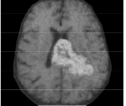
Fig. 1 Brain image with a tumor.
MR Image Characteristics of Brain Tumors:MRI has become firmly established as the premier diagnostic modality for the head [4]. It is most commonly utilized for lesion detection, defining the extent, detection of spread and in evaluation of various residual or recurrent disease. (Vezina[51]) MR – with its multi-planar imaging capabilities, higher end sensitivity to pathologic processes, and excellent anatomic detail – will always be the choice of imaging study in the evaluation of intracerebral tumors if cost and availability were not issues [7]. MRI has better sensitivity for brain tumors compared to CT, both in terms of detection as well as in showing explicitly the extent of the tumor. The major aspect of multi-planar imaging is
itssuperior tumor localization, than just increasing the detection rate of lesions. MRI provides significantly more information about intrinsic tissue characterization and parallels findings on gross pathology. The effects of necrosis on MRI are complex and varied but can often be identified with near-certainty. The association of cysts with certain neoplasms has long been utilized as an aid to differential diagnosis by neuroradiologists and MRI is very good at picking up cysts that are very sharply demarcated, round or ovoid masses. MRI uniquely exhibit hemorrhage, because of the paramagnetic properties of many of the blood-breakdown products. The signal intensity pattern of intratumoral hemorrhage differs from benign intracranial hematomas. Fat-containing neoplasms (e.g., teratoma, dermoid, lipoma) are easily identified or detected on MRI. The dilated and increased blood vessels to the tumors may also be seen well on MRI and magnetic resonance angiography (MRA).
Fig 2 Appearance of tumor in T1-weighted, T1-contrast enhanced and T2-weighted images of the same axial slice
2. Previous Work
Clustering Method
:
Unsupervised techniques, also called “clustering”, need no human intervention and can automatically find the structures in the data. Clustering methods include k-nearest neighborhood (kNN), k-means, fuzzy c-means (FCM), and self-organizing map networks. Velthuizenet al. (1995[9]) proposed a refinement of FCM segmentation by allowing the small classes like tumors to have a noticeable effect on a validity measure, called validity guided clustering, and a genetic algorithm to improve classification from FCM (1996[5]) to segment tumor in 2D. Three data sets (one glioblastoma, one meningioma and one astrocytoma) were tested. The detection rate of meningioma is 76%, gioblastoma 81%, and astrocytoma only 17%. Ahmed et al. (2002[1]) proposed a bias-corrected FCM algorithm (BCFCM) modified by neighborhood field effect. The algorithm was used to compensate for the in homogeneity caused by imperfections in the radio-frequency coils or the problems associated with the acquisition sequences, and allow the labeling of a pixel (voxel) tobe influenced by labels in its immediate neighborhood. In noisy images, the BCFCM technique produced better results than Expectation-Maximization (EM) algorithm. However, it is limited to single-feature inputs, and the algorithm needs further clinical evaluation.Knowledge-based Method:Knowledge-based techniques combine knowledge of anatomy, signal intensity or spatial location of anatomic structures with unsupervised methods. Thompson (Thompson et al, 1998[45]) and Li (Li et al, 1993[27]) suggested aKnowledge-based approach that estimates symmetry of CSF. A tumor can thus be detected only on slices that disturb the CSF spatial symmetry. The measures used were based strictly on predefined intensity thresholds that can vary from one data set to another. Presumingthe tumors appear to have intensity, higher than that of GM on T2-weighted images. Moreover it was applied to 2D images, the symmetry
characteristics of CSF will be influenced, when the collectedaxial slice is not perpendicular to the MSP. Clark et al. (1998[10]) proposed a multispectral analysis tool that segments and labels glioblastoma-multiforme tumor, and compared with kNN. Yoon et al. (1999[55]) used FCM for the initial binary classification of brain, one class is WM and GM, another class is CSF. A symmetry property measures based on the number of pixels, moment invariants and Fourier descriptors were defined to quantify the normality of slices. The related weights for these three parameters were set without any proof and the quantification of normality was performed only on 40 slices in 1 normal and 2 abnormal T2-weighted studies. Lynn et al. (2000[31]) introduced an automatic segmentation of non-enhancing brain tumors based on FCM initial segmentation and image processing techniques controlled by domain knowledge system. Using signal intensity and spatial location of anatomic structures derived from a digital atlas, Michael et al. (2001[10]) proposed an automatic algorithm for tumor segmentation using iterative statistical classification and region growing, which takes 5-10 minutes. Structural and radiometric asymmetry was analyzed through a large deformation image warping in 2D (Joshi et al., 2003[22]). Nine tumors and four normal cases were tested. There is no information on the running time. The second stage of algorithm was based on Christensen’s warping algorithm (Christensen et al., 1996[12]) that is extremely time consuming Christensen, 1994[11]).
Model-based Method:Model-based techniques and deformable models have also been used in tumor detection and segmentation. Capelle et al. (2000[6]) proposed Markov random field model-based unsupervised segmentation in combination with anisotropic filtering and a posterior estimator to segment the brain into homogenous regions to localize possible tumors. Moon et al. (2002[13]) described a model derived from the digital brain atlas containing the spatially varying prior probability maps for the location of WM, GM, CSF, brain tumors and edema. Based on the model, the expectation maximum algorithm is used to remodify the model with individual subject’s information about tumor location, and to segment the tumor and edema. Ho et al (2002[19]) proposed an iterative level-set evolution with a region competition segmentation method with an initialization probability map obtained from intensity-based fuzzy classification.
3. Proposed Approach
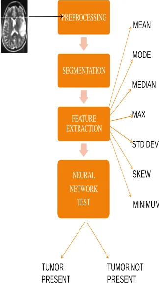
Basically, two main phases are employed in this project which is theoretical phase and practical phase. Theoretical phase involves the process of reading and understanding, reviewing of theories, studying and surveying, classification and detection techniques on medical image fields. There are 4 stages involved in the proposed model which starts from the data input to output. The first stage being the image processing system. Mainly in image processing system, image acquisition and enhancement are steps that need to be done. In this project, these two steps are skipped and all the images are collected from available resources. The proposed model requires converting the image into a format capable of being manipulated by the computer. The MR images are basically converted into matrices form by using MATLAB. The proposed approach mainly contains four steps. This convention makes working with images in MATLAB similar to working with any other type of matrix data, and makes use of the full power of MATLAB available for image processing applications. An intensity image is a data.
PREPROCESSING
SEGMENTATION
FEATURE EXTRACTION
NEURAL NETWORK
TEST
MEAN
MODE
MEDIAN
STD DEV
SKEW MAX
MINIMUM
TUMOR NOT PRESENT TUMOR
PRESENT
Fig 3
Feature extraction involves simplifying the amount of resources required to describe a large set of data precisely. The number of variables involved is one of the major problemwhen performing analysis of complex data.
Analysis when done with a numerous variables generally involves a large amount of memory and/or computation power or a classification algorithm that over fits the training sample and generalizes inadequately to new samples. Feature extraction being a general term for methods of constructing combinations of the variables to get around these problems while still describing the data with sufficient accuracy. Best results are normally achieved when an expert constructs a set of application-dependent features.
Fig 4
4. Result
Table 1 Classification of patientsand brain MRI studies performed
Mean StdDev median Mode Min Max
1 195.13 52.227 216 239 32 255
2 199.594 45.032 234 252 49 255
3 182.336 53.799 215 255 18 255
4 199.931 48.936 237 255 13 255
5 199.377 43.431 222 255 13 255
6 155.42 68.351 216 255 12 255
7 153.504 68.517 256 255 12 255
8 159.171 54.736 289 255 20 255
9 155.781 62.51 234 255 12 255
10 157.355 67.877 231 255 12 255
11 145.304 57.277 265 255 13 255
12 197.183 82.313 253 255 13 255
14 176.616 71.43 198 255 12 255
15 163.779 66.179 196 255 12 255
16 80832 148.747 53.561 255 3 255
17 47428 173.656 57.982 255 5 255
18 184730 199.917 37.096 221 14 255
19 22852 171.825 62.238 255 47 255
20 22138 173.377 64.728 255 32 255
21 29844 204.069 43.011 255 11 255
22 49836 196.743 44.748 236 7 255
23 72824 197.524 61.482 246 32 255
24 26500 203.108 44.34 239 23 255
25 70304 197.119 62.088 245 32 255
26 148.747 53.561 195 255 13 255
27 173.656 57.982 194 255 15 255
28 199.917 37.096 193 221 14 255
29 171.825 62.238 193 255 47 255
30 173.377 64.728 234 255 32 255
31 205.069 43.011 193 255 11 255
32 206.743 44.748 253 236 7 255
33 207.524 61.482 265 246 9 255
34 203.108 44.34 189 239 9 255
35 207.119 62.088 199 245 2 255
36 205.13 52.227 234 239 2 255
37 203.594 45.032 198 252 2 255
38 202.336 53.799 196 255 3 255
39 201.931 48.936 194 255 3 255
40 204.377 43.431 193 255 2 255
Table 2 Classification of patientsand brain MRI Test tumor
Mean Median StdDev Mode Min Max
223.008 180 41.85 255 19 255
238.215 229 61.33 246 30 255
214.322 172 54.787 255 8 255
219.849 230 47.593 231 20 255
202.189 171 54.594 255 9 255
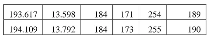
Table 3 Classification of patientsand brain MRI Test Non-tumor
Mean StdDev Mode Min Max Median
175.597 16.014 165 136 251 173
204.386 9.614 201 144 255 203
193.553 13.535 183 171 252 189
193.617 13.598 184 171 254 189
194.109 13.792 184 173 255 190
5.
Conclusion
Here the output will be in the form of 1 and 0. For nontumor images the output will be 0 and for tumor image output will be 1. We can see the output in the output data of network data manager. In the testing data I have used 5 tumor image and 5 non tumor image .Hence the output data gives the output in 5 column form.
The proposed algorithm shows an effective method for detection of the brain tumors in the 2 dimensional MRI in the various types of image formats like jpeg, bmp formats. This method is much faster than other existing method for detection of tumor. Accuracy of result is depends on the selection of input image having boundary of tumor region and also size of the tumors which have got grown in the tissues.
References
[1] M. Celenk, “A Color Clustering Technique for Image Segmentation,” Computer vision, Graphics and Image Processing, vol. 52, pp. 145-170, 1990.
[2] Y. I. Ohta, T. Kanade, and T. Sakai, “Color Information for Region Segmentation,” Computer Graphics and Image Processing, vol. 13, pp. 222-241, 1980.
[3] S. E. Umbaugh, “Computer vision in medicine: Color metrics and image segmentation methods for skin cancer diagnosis,” Ph.D. dissertation, Dept. of Electrical Engineering, University of Missouri-Rolla, MO,1990.
[4] F. Ercal, A. Chawla, W. V. Stoecker, and R. H. Moss, “Diagnosing Malignant Melonoma Using a Neural Network,” Intelligent Engineering Systems Through Arrificial Neural Networks, vol. 2, ASME Press, pp.
[5] J. E. Golston, R. H. Moss, and W. V. Stoecker, “Boundary Detection in Skin Tumor Images: An Overall Approach and A Radial Search Algorithm,” Pattern Recognition, vol. 23, no. 11, pp. 1235-1247, 1990.
[6] P. A. Dhawan and A. Sicsu, “Segmentation of images of skin lesions using color and texture information of surface pigmentation,” Computerized Medical Imaging and Graphics, vol. 16, pp. 163-177, May 1992.
[7] S. E. Umbaugh, R. H. Moss, and W. V. Stoecker, “An automatic color segmentation algorithm with application to identification of skin tumor borders,” Computerized Medical Imaging and Graphics, vol. 16, pp.227-235, May 1992. [8] A. Rosenfeld and A. C. Kak, Digital Picture Processing, 2nd
ed., vol. I. Orlando, FL: Academic Press, 1982, pp. 261-264. Richard 0. Duda and Peter E. Hart, Pattern Classijication and Scene Analysis New York Wiley, 1973, pp. 290-292. [9] J. E. Golston, W. V. Stoecker, R. H. Moss, and I. P. S.
[10] Ahmed M.N., Yamany S.M., Mohamed N., Farag A.A., Moriarty T., “A modified fuzzy c-means algorithm for bias field estimation and segmentation of MRI data”. IEEE Trans Medical Imaging, 21(3), 193-199, 2002.
[11] Christensen G.E., “Deformable shape models for anatomy”. Electrical Engineering D.Sc. Dissertation, Washington University, St. Louis, Missouri, 1994.
[12] Christensen G.E., Rabbit R.D., Miller M.I., “Deformable Templates Using Large Deformation Kinematics”. IEEE Trans Medical Imaging, 5(10), 1435-1447, 1996.
[13]Cocosco C.A., Kollokian V., Kwan R.K.S., Evans A.C., “BrainWeb: Online Interface to a 3D MRI Simulated Brain Databas. NeuroImage”.3rd International Conference on Functional Mapping of the Human Brain HBM 97, Copenhagen, 4(2-4), S425 – Proc. 1997.
[14]David G. S., Richard O. D., Peter E. H., Pattern Recognition. [15]Denoeux T., “A k-nearest neighbor classification rule based
on Dempster-Shafer Theory”. IEEE Trans. Systems Man Cybernet.25 (5), 804-813, 1995.
[16] Edward A.A., Chihiro T., Michel J.B., Andrew G., Saara T., Sven E., “Accuracy and reproducibility of manual and semiautomated quantification of MS lesions by MRI”. Journal of Magnetic Resonance Imaging, 17(3), 300-308, 2003.
[17] AnantBhardwaj,Kapil Kumar Siddhu,” An Approachto Medical Image Classification Using Neuro Fuzzy Logicand ANFIS Classifier, International Journal of Computer Trends and Technology –volume 4 Issue 3-2013.
ShrikantBurjehas received degrees B.E (Electronics and Tele) and M.E. (Electronics) from Amravati University,Maharashtra State, India in 1997 and 2003 respectively. He is presently working as Assistant Professor in the Department of Electronics, RCET Bhilai Chhattisgarh State, India. He is a member of professional bodies like Indian society of technical Education and Institution of Engineers. His research interests include Medical Image processing and soft computing techniques.
Dr. SourabhRungta received his M. Tech.
(Computer Technology) degree in 2002 from NIT Raipur, (India). Presently he is working as Professor at