DOI: 10.15662/ijareeie.2014.0307002
Natural Space Vector Modulation in Six-Step
Voltage Source Inverters
R.De Four
1, T.Wadi
2Lecturer, Dept. of ECE, The University of the West Indies, St. Augustine, Trinidad, WI 1 PT Lecturer, Dept. of ECE, The University of the West Indies, St. Augustine, Trinidad, WI2
ABSTRACT:This paper presents the existence of natural space vector modulation occurring between adjacent switching space vectors in quasi-square wave voltage source inverters. This natural space vector modulation is responsible for the hexagonal trajectory of the rotating resultant voltage space vector which is produced by the referral of the instantaneous line or phase voltage quantities to the drive’s virtual magnetic axes. Space vector rotation, which gives rise to the hexagonal trajectory only occur between switching states when the instantaneous line or phase voltages are undergoing changes in magnitude. The theoretical approach undertaken to develop the concept of natural space vector modulation is also supported with experimental results and fully support the well-known theory of space vector modulation.
KEYWORDS:Natural, Space Vector Modulation, Voltage Source Inverter.
I.INTRODUCTION
Voltage source inverters (VSI) have been widely used in the production of three-phase non-sinusoidal quasi-square wave voltages and vector analysis has also been applied to the analysis of these inverters [1, 2]. The production of sinusoidal waveforms from these inverters has been accomplished with the familiar space vector modulation approach [3 – 5] which was applied to a three-phase unity power factor ac to dc converter by Busse and Holtz [6]. The space vector modulation (SVM) technique modulates the adjacent stationary switching space vectors of a quasi-square wave drive to produce a variable voltage and variable frequency sinusoidal output, with the rotating resultant voltage space vector displaying a circular trajectory. However, the trajectory of the resultant voltage space vector produced by a quasi-square inverter has been reported to be hexagonal in nature [2, 7] with little emphasis being placed onits origin. In addition, the choice of using line or phase quantities in the production of the resultant switching space vectors of a quasi-square wave drive and the magnetic axes with which they are referred, have not been elaborated on in the literature.
This paper examines the line and phase voltages and their corresponding switching space vectors produced by a quasi-square wave voltage source inverter. Virtual line and phase voltage magnetic axes are introduced and the relationship between line and phase voltage switching space vectors is presented. The process of natural modulation of adjacent switching space vectors of a quasi-square wave drive and the conditions for this natural modulation to occur is developed and supported with experimental results.
II. RELATED WORK
The foundation of vector representation of three-phase systems was laid by Park [8] and Kron [9], and the application of the vector method to the analysis of electrical machines was presented by Kovacs and Racz [10]. They developed transient mathematical models of electrical machines and displayed the physical phenomenon occurring in these machines.The vector method is now widely used in the analysis of voltage source space vector modulated inverters.
III. INVERTER SWITCHING STATES
DOI: 10.15662/ijareeie.2014.0307002 The inverter consists of six transistors Q1to Q6, accompanied with their respective anti-parallel diodes D1to D6.Each
inverter leg feeds the star connected balanced load from the collector-emitter connections labeled A, B and C. The inverter is fed with a supply voltageVdcfrom the filter capacitor and a DSP is utilized to control the switching of the
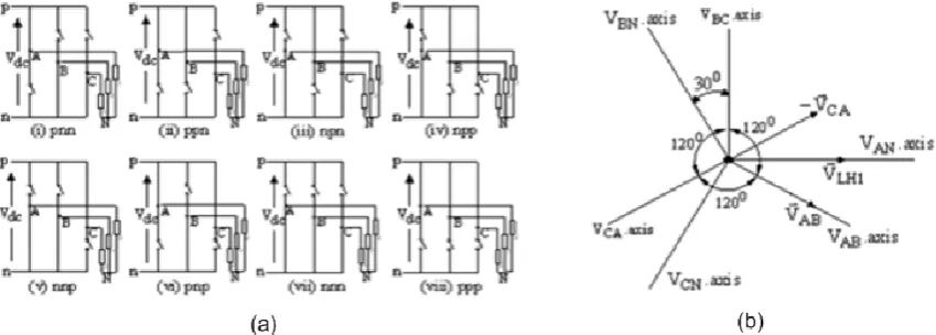
transistors. The operating constraints of this inverter must ensure that two transistors in an inverter leg are not turned on at the same time and the output current of the inverter must always be continuous. These constraints yield eight possible operating states of the inverter. Six of these states produce a non-zero output voltage and are called non-zero switching states, while the other two produce zero output voltage and are known as zero states [2, 7, 5, 11, 12]. The eight switching states are shown in Figure 2(a).
Figure 1 Three-phase Voltage Source Inverter
The switching sequence shown in (i) to (vi) of Figure 2(a), has been used to produce a three-phase output voltage from the inverter. The switching sequence begins with the upper switch of leg A and the lower switches of legs B and C turned on. Since the upper switches are connected to p, the positive of the filter capacitor and the lower switches to n, the negative of the filter capacitor, this state is designated aspnn. Each subsequent state is produced by switching the pair of transistors in one leg of the inverter.
The sequence from states (i) to (vi) and back to (i) of Figure 2(a) is produced by switching transistors in legs B, A, C, B, A and C. Since there are six active switching states in a cycle, then each switching state spans for T/6 seconds, where T is the period of the output line voltage waveform.
Figure 2. (a) Eight Switching States of the Voltage Source Inverter (b) Line and Phase Voltage VirtualMagnetic Axes and ResultantLine SSVs for State pnn.
IV. LINE VOLTAGE SWITCHING SPACE VECTORS
DOI: 10.15662/ijareeie.2014.0307002 VAB, VBC, and VCA, each being 120° out of phase with the other in the given sequence. The line voltages produced by
the switching state in Figure 2(a)(i) are given by:
VAB = Vdc, VBC = 0, VCA = -Vdc. (1)
Figure 4 (i) Inverter Output Voltage Waveforms. (a) Quasi-Square Wave Line Voltage Waveforms(b) Six-Step Phase Voltage Waveforms. Figure 4(ii). Line and Phase Switching Space Vectors and Virtual Magnetic Axes
As stated by Kovacs [13], the resultant line voltage vector of a three-phase system of voltages fed to a three-phase stator of a motor is given by:
(2)
Similarly, the resultant line voltage vector of a three-phase system of voltages delivered by the three-phase stator of a generator is also given by Eq. (2). The resolution of𝑉 L, along the line voltage magnetic axes, produces the
instantaneous line voltages of the three-phase system. Taking Eq. 2 to represent the resultant line voltage vector produced by the three-phase voltage source inverter of Figure 1, and representing the vectors in Eq. (2) by their instantaneous values and the spatial position of the line voltage virtual magnetic axes results in
(3)
where VAB, VBC, and VCA, are the instantaneous line voltage magnitudes and exp(-j30), exp(j90) and exp(j210) are the
respective spatial position of the line voltage virtual magnetic axes of the three-phase system produced by the voltage source inverter. Substituting the instantaneous voltages of Eq. (1) in Eq. (3) yields:
(4)
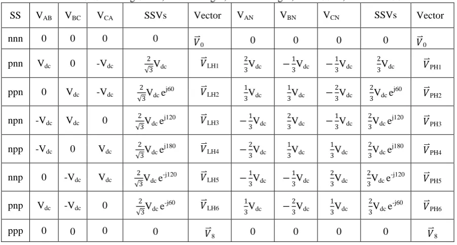
The line and phase voltages virtual magnetic axes of the three-phase system of voltages, produced by the three-phase inverter of Figure 1, line voltage vectors, and their resultant for switching state pnn are shown in Figure 2(b).
DOI: 10.15662/ijareeie.2014.0307002 the instantaneous phase and line voltages are located along the magnetic axes of a three-phase stator [13, 14], then, the instantaneous phase and line voltages of the voltage source inverter of Figure 1 will lie along its virtual magnetic axes as shown in Figure 2(b).The application of the above procedure to the other five non-zero and the two zero switching states in Figure 2(b), produces the line voltage switching space vectors, 𝑉 LHKas shown in Table 1, where k=1,2....6.The
three-phase inverter line voltage waveforms and the resulting line voltage switching space vectors obtained from Table 1 are shown in Figures4(i) and Figure 4(ii) respectively.
Table 1 VSI Switching States, Line Voltages, Phase Voltages, Line SSVs, and Phase SSVs
SS VAB VBC VCA SSVs Vector VAN VBN VCN SSVs Vector
nnn 0 0 0 0 𝑉
0 0 0 0 0 𝑉 0
pnn Vdc 0 -Vdc
2
3Vdc 𝑉 LH1
2
3Vdc −
1
3Vdc −
1 3Vdc
2
3Vdc 𝑉 PH1
ppn 0 Vdc -Vdc
2 3Vdc e
j60 𝑉 LH2
1 3Vdc
1
3Vdc −
2 3Vdc
2 3Vdc e
j60 𝑉 PH2
npn -Vdc Vdc 0
2 3Vdc e
j120 𝑉
LH3 −
1 3Vdc
2
3Vdc −
1 3Vdc
2 3Vdc e
j120 𝑉 PH3
npp -Vdc 0 Vdc
2 3Vdc e
j180 𝑉
LH4 −
2 3Vdc
1 3Vdc
1 3Vdc
2 3Vdc e
j180
𝑉 PH4
nnp 0 -Vdc Vdc
2 3Vdc e
-j120 𝑉
LH5 −
1
3Vdc −
1 3Vdc
2 3Vdc
2 3Vdc e
-j120
𝑉 PH5
pnp Vdc -Vdc 0
2 3Vdc e
-j60 𝑉 LH6
1
3Vdc −
2 3Vdc
1 3Vdc
2 3Vdc e
-j60 𝑉 PH6
ppp 0 0 0 0 𝑉 8 0 0 0 0 𝑉 8
The line voltage switching space vectors produced by the three-phase quasi-square waves of Figure 4(i)(a), are all of constant magnitude(2/ 3)𝑉dc and each exist for a time equal to about T/6 seconds, where T is the period of the waveforms. The six non-zero resultant line voltage space vectors are represented by the general expression:
for k = 1, 2,…6 (5)
V.ROTATION OF LINE VOLTAGE SPACE VECTORS
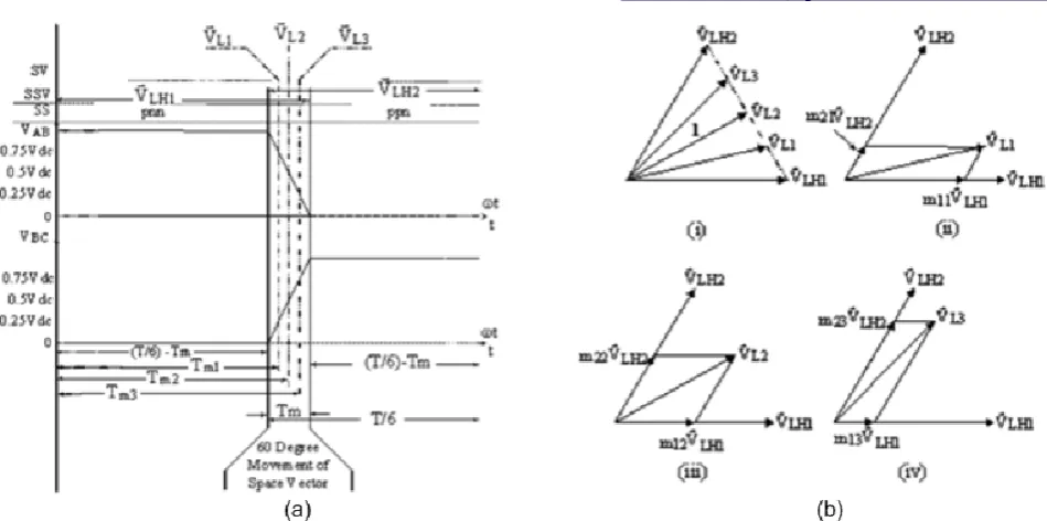
The line voltage switching space vectors𝑉 LHK shown in Figure 4(ii) are stationary space vectors, each occupying a fixed
position in space. Figure 4(i)(a) shows that each switching space vector is active for about T/6 seconds and they are produced in the sequence𝑉 LH1, 𝑉 LH2 through𝑉 LH6. The fall of VAB fromVdc to zero and the rise of VBC from zero toVdc,
results in the decay of switching space vector𝑉 LH1 and the growth of switching space vector𝑉 LH2. Assuming that the
rate of fall of VAB is equal to the rate of rise of VBC, the natural rotation of the resultant voltage space vector within
sector 1 can be examined. Since the production of switching space vector𝑉 LH2 follows that of𝑉 LH1 and is accomplished
by the switching of the two transistors in leg B of the inverter, only waveforms VABand VBCwill be examined in the
interval of concern, because waveform VCAis unaffected by the leg B switching. Figure 6(a) examines the VAB andVBC
DOI: 10.15662/ijareeie.2014.0307002
Figure 6(a). VAB and VBC Waveforms for Production of 𝑉 LH1 and 𝑉 LH2 During Linear Fall of VAB andRise of
VBCFigure 6(b). Switching and Rotating Space Vectors (i) SSVs andThreeRotating Space VectorsDuring Tmin Sector1
(ii) Components of𝑉 L1 (iii) Components of𝑉 L2 (iv) Components of𝑉 L3
For the interval examined in Figure 6(a), line voltage VCAis unchanged and its value is -Vdc. Three values of line
voltages VAB and VBC have been recorded in the time interval Tm of Figure 6(a), when these voltages are changing from
their old to new values. For times indicated by Tm1, Tm2 and Tm3, all taken in Tm, the corresponding line voltages are:
Time = Tm1, VAB = 0.75Vdc VBC = 0.25Vdc, VCA = -Vdc (6)
Time = Tm2, VAB = 0.5Vdc VBC = 0.5Vdc, VCA = -Vdc (7)
Time = Tm3, VAB = 0.25Vdc VBC = 0.75Vdc, VCA = -Vdc (8)
The resultant line voltage vectors at times Tm1, Tm2 and Tm3 are obtained by substituting Eqs. (6), (7) and (8) into Eq.
(3) and are given by:
𝑉 L1 = 1.0408Vdce j13.9
(9)
𝑉 L2 = 1.0Vdcej30 (10)
𝑉 L3 = 1.0408Vdcej46.1 (11)
The two adjacent switching space vectors in this transitional time Tmare𝑉 LH1and 𝑉 LH2, where:
𝑉 LH1 = 1.1547Vdcej0 (12)
𝑉 LH2 = 1.1547Vdcej60 (13)
The five space vectors in Eqs. (9), (10), (11), (12), and (13) when plotted in the complex plane is shown in Figure 6(b)(i). The three space vectorsare𝑉 L1, 𝑉 L2and 𝑉 L3 in Figure 6(b)(i) can be resolved along the switching space vectorsare𝑉 LH1 and 𝑉 LH2 as shown in Figures 6(b)(ii) to 6(b)(iv) respectively.
The two switching space vectorsare𝑉 LH1and 𝑉 LH2 are active during this time interval Tm, when VABis falling linearly
and VBCis rising linearly as shown in Figure 6(a). Hence, the resultant voltage space vectors 𝑉 L1, 𝑉 L2 and𝑉 L3 that are
produced in the interval Tm, must comprise of fractions of switching space vectors 𝑉 LH1and 𝑉 LH2. This is reflected in
Figures 6(b)(ii) to 6(b)(iv), where the fractions of𝑉 LH1 and𝑉 LH2 used in the production of resultant voltage space vectors
𝑉 L1 are indicated by m1i𝑉 LH1 andm2i𝑉 LH2respectively, where i = 1...3. Hence, the switching space vectors𝑉 LH1 and𝑉 LH2are
modulated naturally during the interval Tmto produce a resultant voltage space vector that rotates through the angle 𝜔𝑡 = 600formed by sector 1. It must be noted that during the time intervals T/6 – T
mthat accounts for almost 600 along
DOI: 10.15662/ijareeie.2014.0307002 are fixed in space for that time. It is only during the short time interval of Tmwhen the line voltage magnitudes are
changing, that rotation of the resultant voltage space vector occurs as shown in Figure 6(a). Hence, the 600 movement along the line voltage waveforms is represented by the 600sectors forming the hexagon of Figure 4(ii), and the time taken by the resultant voltage space vector to traverse this 600sector is denoted by Tm. Therefore, space vector rotation
only occurs when the voltages from which they are produced are undergoing changes in magnitude. During one cycle of operation, the resultant line voltage space vectorV L rotates through 3600and having a trajectory of the line voltage hexagon of Figure 4(ii), when the voltage source inverter of Figure 1 is driving a balanced star-connected unity power factor load.
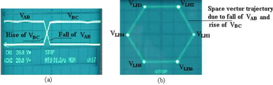
Figure 7(a) is an oscilloscope picture showing the fall of line voltage VABand the rise of VBCduring Tm, while, Figure
7(b) shows a picture of the trajectory of resultant line voltage space vector 𝑉 L.
The theory of space vector modulation as presented in [3 – 5] performs forced modulation on the adjacent switching space vectors to achieve a circular trajectory of the resultant voltage space vector in the production of sinusoidal voltages from quasi-square wave line voltage waveforms. However, the production of a hexagonal trajectory produced by the resultant voltage vector of a quasi-square wave inverter, reveals that adjacent stationary switching space vectors were modulated naturally due the fall and rise of line voltages, thereby producing a rotating resultant voltage vector whose trajectory is a hexagon.
Figure 7. Space Vector Rotation Due to Natural Modulation of SSVs. (a) Fall and Rise of Line Voltage Waveforms VABand VBCRespectively (b) Trajectory of Line Voltage SSVs by Natural Modulation of Adjacent SSVs
VI.PHASE VOLTAGE SPACE VECTOR
The load phase voltages VAN, VBNand VCN, for the eight switching states in Figure 2(a) are obtained using the three line
voltages produced for each state. These phase voltages are recorded in Table 1 and their waveforms are plotted in Figure 4(i)(b). Examination of the phase and line voltage waveforms in Figure 4(i) reveals that the phase voltage lags the line voltage by 30°, thus resulting in the 30° phase shift between the line and phase voltage virtual magnetic axes of Figure 2(b). In addition, the phase voltage waveforms of Figure 4(i)(b) are six-step voltage waveforms, since there are six voltage steps in a cycle. Employing [13], the resultant phase voltage vector of a three-phase system is given by,
𝑉 P = 2/3(𝑉 AN + 𝑉 BN + 𝑉 CN). (14)
Representing the vectors in Eq. (14) by their instantaneous values and the spatial position of the phase voltage virtual magnetic axes yields,
𝑉 P = 2/3(VAN + VBN ej120 + VCN ej240). (15)
whereVAN, VBNand VCN are the instantaneous phase voltage magnitudes and ej120 and ej240 are the respective spatial
DOI: 10.15662/ijareeie.2014.0307002
k = 1, 2, …6 (16)
for the six non-zero resultant phase voltage switching space vectors. The resultant phase voltage switching space vectors obtained from Figure 2(a) are shown in Figure 4(ii) and presented in Table 1.
From Table 1, it is observed that the line voltage switching space vectors are 3 times their phase counterparts, but both line and phase voltage switching space vectors occupy the same position in space, however, their virtual magnetic axes are displaced by 30° from each other. This indicates that either line or phase voltage analysis can be performed and conversion from one to the other is effected by a factor of 3. This is reflected in the resultant line and phase voltage switching space vectors of Eqs. (5) and (16).
VII. CONCLUSION
This paper presented the existence of natural space vector modulation, which is responsible for space vector rotation within the sectors of the hexagon produced by the resultant voltage space vector of a quasi-square wave or six-step voltage source inverter drive. The existence of this natural space vector modulation was supported with experimental results. The issue of virtual magnetic axes was also presented as a means of producing the resultant voltage space vector of a voltage source inverter drive. It was shown that the well known space vector modulation technique, utilizing adjacent switching space vectors to synthesize variable voltage and frequency sinusoidal waveforms from a voltage source inverter, obtained its origin from the natural modulation process that occurred in a quasi-square wave or six-step voltage source inverter drive.
REFERENCES
[1] Holtz, J.,“Pulsewidth Modulation for Electronic Power Conversion,” Proceedings of the IEEE, Volume: 82, Issue: 8, pp. 1194-1214, 1994. [2] Sasi, D., and Kuruvilla, J., “Modelling and Simulation of SVPWM Inverter Fed Permanent Magnet Brushless DC Motor Drive,” IJAREEIE Vol. 2, Issue 5, pp. 1947-1955, May 2013.
[3] Bose, B. K.,“Power Electronics and Variable Frequency Drives: Technology and Applications,” IEEE Press, New York, p. 159, 1997. [4] Rashid, M. H.,“Power Electronics: Circuits, Devices and Applications,” Pearson Prentice Hall, New Jersey, p. 271, 2004.
[5] HimamshuPersad, V.,“Analysis and Comparison of Space Vector Modulation Schemes for Three-leg and Four-leg Voltage Source Inverters,” Master of Science Thesis, Virginia Polytechnic Institute and State University, 1997.
[6] Busse, A., and Holtz, J.,“Multiloop Control of a Unity Power Factor Fast-Switching AC to DC Converter,” IEEE Power Electronics Specialists Conference, Cambridge/Ma., pp. 171-179, 1982.
[7] Altay, S., and Gungor, S., “Analysis and Comparison of Space Vector Modulation Schemes for Inverter with Sinusoidal Output Current by Using DSP Controller,” Istanbul Technical University, Faculty of Electrical & Electronic, Dept. of Electrical Engineering, Istanbul, Turkey. [8] Park, R.H., “Two-Reaction Theory of Synchronous Machines”, AIEE Trans. No.48, 1929, pp.716-730 and no. 52, pp.352-355, 1933. [9] Kron, G., “The Application of Tensors to the Analysis of Rotating Electrical Machinery”, Schenectady, NY, USA, General Electric Review, 1942.
[10] Kovacs, K.P., and Racz, I., “TransienteVorgange in Wechselstrommachinen”, Budapest, Hungary, Akad.Kiado, 1959.
[11] Bandana, Banupriya, K., Subrahmanyam, JBV., Sikanth, Ch., M.Ayyub, M., “Space Vector PWM Technique for 3phase Voltage Source Inverter Using Artificial Neural Network,” IJEIT, Vol. 1, Issue 2, February 2012.
[12] Neacsu, D. O., “Space Vector Modulation – An Introduction,” The 27th Annual Conference of the IEEE Industrial Electronics Society, 2001. [13]Kovacs, P. K.,“Transient Phenomena in Electrical Machines,” Elsevier Science Publishers, 1984.
[14]De Four, R., “A Self-Starting Method and an Apparatus for Sensorless Commutation of Brushless DC Motors,” WIPO Publication No. WO 2006/073378 A1, 2006.
BIOGRAPHY
Ronald De Four received his PhD, MPhil and BSc degrees in Electrical and Computer Engineering from The University of the West Indies, St. Augustine, Trinidad. Presently, he is a Lecturer in the Department of ECE, UWI, Trinidad. His area of interest include power electronics, variable speed drives and solar power systems.