A Case Study: 2D Vs 3D Partial Differential
Equation toward Tumour Cell
Visualisation on Multi-Core Parallel
Computing Atmosphere
Md. Rajibul Islam1, Norma Alias2 1
Faculty of Information Science and Technology, Multimedia University, Malaysia 2
Ibnu Sina Institute, Faculty of Science, University Technology Malaysia, Johor E-mail: [email protected], [email protected]
Abstract
This study thrashes out some of the visualisation and computational challenges encountered in the field of neuroscience. With the intention to address such computational challenges; we recognised the particular significance of the iterative solvers and parallel algorithms on Multi-Core parallel computing atmosphere. In order to detect tumour cells, 2D and 3D Partial Differential Equations (PDE) are considered and compared by using Multi-Core parallel computing atmosphere with visualisation, communication and data analysis. The performance analysis of Multi-Core computing is presented in provisions of speedup, efficiency, effectiveness and temporal performance where the use of 2D and 3D PDEs and parallel algorithms was found to give in remarkable results.
Keywords: PDE (Partial Differential Equation), tumour cell, Multi-Core computation
1. INTRODUCTION
The simulation of human tumour growth by parallel algorithm is the latest invention nowadays. A brain tumour is an abnormal growth of cells without any specific order, with the disability to control their growths within the brain or inside the skull, which can be cancerous or non-cancerous. Brain tumours are the leading causes of death by cancer. From a case study reported in an ABC news report, it was found that among 36 people, 1.6% of them suffered from brain tumour and the rate is increasing currently. Therefore we propose intervention measures be implemented by the early prediction of brain tumour growths. In this study, the monitoring and visualisation of the growth of tumour cells are performed by large scale mathematical simulation. The tools of 2D and 3D parabolic type partial differential equations are accented as the computational engine for the future prediction of the cell growth. Clinical data provides the initial and boundary information on the properties of tumour.
interface that enables the visualisation of the reconstructed 3D prostatemodel including all internal anatomical structures and their relationships to define tumour volumeand distribution and pathways of needle biopsies. Thus it has improvedthe understanding of prostate cancer behaviour and current diagnosis-staging methodology. In addition, Lang et al. (1999) described an optimisation process specially designed for regional hyperthermia of deep-seated tumours in order to achieve desired steady-state temperature distributions. A nonlinear three-dimensional heat transfer model based on temperature-dependent blood perfusion was applied to predict the temperature. They obtained optimal heating by minimising an integral objective function which measures the distance between desired and model predicted temperatures.
The authors’ previous work represents a new efficient and dynamic solvers for the numerical solutions of partial differential equations (PDEs) in order to visualise tumour cell through distributed high performance computing (Norma et al., 2009a and 2009b). A comparative case study in terms of the visualisations, performance analysis of 2D and 3D parabolic type partial different equations using multi-core parallel computing atmosphere is presented in this paper. This paper is organised as follows. In section 2, mathematical model of 2D and 3D parabolic PDEs and discretisation of the model was presented, multi-core parallel computing system was illustrated in section 3, 2D and 3D tumour cell visualisation was displayed in section 4. And section 5 presented the performance analysis and discussion of multi-core computing system and finally, section 6 concludes the paper.
2. THE MATHEMATICAL MODEL
The model represents both the avascular and the vascular phase of tumour evolution, and is able to simulate the time when the transition occurs. The evolution problems can be written as a free-boundary problem in parabolic type joined with an initial-boundary value problem in a fixed domain. Cell populations and chemical species are the model dependent variables that distinguish the physical status of the biological scheme in both the tumour mass and the outer environments. They are fundamentally different. The cell size is much larger than that of the chemical factors and macromolecules. The cells are surrounded by a membrane and cannot go through each other; they occupy definite physical space. Comparatively, the chemical species consist of macromolecules that may spread in the intercellular space, are able to attach to the cell membrane or go through it, such that they actually do not take up physical space (Hogea et al., 2006). The cell populations are considered important for the process and the chemical factors that influence their motion and proliferation (Preziosi, 2004).
We have considered the fundamental mathematical model, developed by Angelis & Preziosi (2000) which describes the diffusion of cancer cells through brain tissues. The parameter estimation of the model, the growth rate and the diffusion coefficient will be discussed and the simulation for brain tumour growth is done by the following parabolic partial differential equation general balance law in local form as discussed by researchers such as Angelis & Pre ziosi (2000), Bellomo & Presiosi (2000), Preziosi (2004), Ambriosi & Preziosi (2002) and Hogea et. Al. (2006) as below:
(1)
Where: Γ = Γ(u) is the generation (proliferation / production) coefficient Lu
u Q u
W +∇ ∇ +Γ−
∇
− . ( ) .( )
=
∂
∂
L = L (u) is the death / decay coefficient of the cells
Q is the diffusion coefficient
W is the drift velocity field.
The model that was represented in this study is an extension to their model from W = (P, R) (two dimensions) to W = (P, R, S) (three dimensions)
Hence, the brain tumour growth can be written mathematically in 2D and 3D form as illustrated below. The parameter estimation of the model, the growth rate and the diffusion coefficient were presented and the simulation for brain tumour growth was done by the 2D and 3D PDEs equation below. The results of the simulations was visualised by graphical presentation and comparisons were made to obtain better solution for the challenging tumour cell visualisation problem:
Two-dimensional (2D) parabolic equation
The mathematical model consists of an evolution equation for the variable u=u( xt, )which was considered to describe, in time, t and space, x, the physical state of the system. The variable u includes both the cell population and chemical factors produced in the environment by the interacting cells. The derivation of the model here described is developed on the basis of mass balance equations, and are supported by a random walk scheme (Bellomo & Preziosi, 2000).
Under suitable regularity assumptions one can expand the use of N,P,Qand R , as well as the use of Ni,j(t)≈u(t,xi,yj)∆Vi,j, and represent the word equation above mathematically (Angelis
& Preziosi, 2000) from equation (1), we derived 2D mathematical model as:
Lu y u y Q y u Q x u x Q x u Q y Ru x Pu t u − Γ + ∂ ∂ ∂ ∂ + ∂ ∂ + ∂ ∂ ∂ ∂ + ∂ ∂ + ∂ ∂ − ∂ ∂ − = ∂ ∂ 2 2 2 2 ) ( )
( (2)
With Γ(t,xi,yj)=Γi,j(t)/∆Vi,j and where the indices (i, j) have been substituted with the dependence of u and of all coefficients on the space variable. The elementary volume centred in the node (i, j) is denoted by V and its volume by i,j ∆Vi,j. Finally, all cells inV are i,j considered as concentrated in the node (i, j). While the number of a certain type of cells (or chemical factors) is denoted by Ni,j(t found in the node (i, j) at the time t. )
Three-dimensional (3D) parabolic equation
By using finite difference method with certain assumptions, and by the use of the lattice scheme, we will obtain the three dimensional parabolic equation of the tumour growth. From equation (1), we derived 3D mathematical model as:
Lu z u z Q z u Q y u y Q y u Q x u x Q x u Q z Su y Ru x Pu t
u +Γ−
A. The Discretisation of the 2D and 3D Model Equations
Based on central finite difference method, the discretisation is shown as follow,
Red Black Gauss-Seidel algorithm was implemented with the parallel algorithm in solving the 2D parabolic equations for brain tumour visualisation as,
t t N t t N k ij k ij ∆ − ∆ +
+1)( ) ( )() ( )] ( ) ( [ )] ( ) (
[Pij1Ni(k1,1j) t −PijNij(k) t + Rij 1Ni(,kj11) t −RijNij(k) t
= + − − + − −
+[Qij−1Ni(−k1+,1j)(t)−(Qij−1+Qij+1)Nij(k)(t)+Qi+j1Ni(+k1)j(t)]
+[(Qij−1Ni(,kj+−11)(t)−(Qij−1+Qij+1)Nij(k)(t)+Qij+1Ni(,kj+)1(t)] +Γij −LijNij(k)(t). (4)
In order to solve the parabolic equations for 3D, we need to first discretise the model by using central finite difference method. We have applied the Explicit Method Finite-Difference scheme to perform discretisation of the model and obtain the discretised model as,
t
t N t t
Nijk ijk
∆ − ∆ + ) ( ) ( = − Γ + + + − + + + − + + + − + − + − + − + + + − − − + + + − − − + + + − − − − − − − − − ) ( )] ( ) ( ) ( ) ( [ )] ( ) ( ) ( ) ( [ )] ( ) ( ) ( ) ( [ )] ( ) ( [ )] ( ) ( [ )] ( ) ( [ 1 , , 1 1 1 1 , , 1 , 1 , 1 1 1 , 1 , 1 , , 1 1 1 1 , , 1 1 1 , , 1 , 1 , 1 , , 1 1 t N L t N Q t N Q Q t N Q t N Q t N Q Q t N Q t N Q t N Q Q t N Q t N S t N S t N R t N R t N P t N P ijk ijk ijk k j i j k i ijk j k i j k i k j i j k i k j i j k i ijk j k i j k i k j i j k i k j i j k i ijk j k i j k i k j i j k i ijk j k i k j i j k i ijk j k i k j i j k i ijk j k i k j i j k i (5)
We have formulated the discrete model that involves the use of a discretised form of the PDEs. The entire fixed computational domain 0 ≤ x ≤ 1 and 0 ≤ y ≤ 1 are each discretised by using equally spaced meshes, the interface is a mesh point, corresponding both to x = 1 and y = 1. The domain occupied by the tumour is embedded into a larger fixed, time-independent, computational domain D that is discretised by using a uniform Cartesian mesh with∆x=∆y=h.
3. MULTI-CORE PARALLEL COMPUTING SYSTEM
Two or more independent cores are combined into a single package composed of a single integrated circuit (IC), called a die, or more dies packaged together into a multi-core processor. It is available nowadays as dual-core or quad-core processor, where a dual-core processor holds two cores, and a quad-core processor holds four cores. Multiprocessing are executed by a multi-core processor in a single substantial package. We have implemented multi-core parallel computing system in support of the performance evaluation of 2D and 3D Partial Differential Equations to detect brain tumour in this study, because multi-core parallel computing system is an execution of the same task on multiple cores in order to obtain results/output faster. Besides, the selection, aggregation and sharing of distributed resources provides the infrastructure to solve distributed problem in real life implementation based on their cost, availability, users’ quality, and performance of service requirements. Multi-core parallel computing systems demonstrate enhanced responsiveness due to multitasking with several cores available (Alfredo et al., 2007). A single coherent cache might be shared by cores at the highest on-device cache level or may have separate caches and the same communication is also shared by the processors to the rest of the system. All “core” autonomously execute optimisations such as pipelining, superscalar execution, and multithreading.
In this study, we have used some multi-threaded software such as Wolfram gridMathematica and COMSOL multiphysics in order to evaluate the performances and visualisations. For multi-threaded software, multi-core parallel computing system can distribute considerable performance benefits by adding processing power with least latency. The major reimbursements will be perceived in applications such as customer relationship management, e-commerce, larger databases and virtualisations. The multi-threaded software splits our large application’s data set into smaller pieces that can be executed on in parallel and after the data has been processed, it is combined back into a single data set again to obtain the required results. Through our performance analysis we have proved that, the multi-core machine can handle such kind of parallel tasks more efficiently.
4. 2D AND 3D TUMOR CELL VISUALISATION
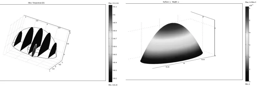
With COMSOL Multiphysics v3.4, we have performed Partial Differential Equation (PDEs) with Finite Element Method simulations on Multi-Core parallel computation atmosphere. A heat transfer coefficient of 5 W/m2 K is used as a convective boundary condition at the skin surface to account for natural convection.
Fig. 1: 3D sub-domain model of tumour cell visualisation that were vertically sliced.
5. PERFORMANCE ANALYSIS AND DISCUSSION
Current processor architectures only feature 2 to at most 4 cores per processor. We therefore use 8 processors with dual-core each with IBM POWER5 shared-memory PCs for our experiments, which we believe most closely resembles our target designs. Unless otherwise noted, we use all 16 cores in our tests.
A. Sequential programming analysis
Based on the computation of our sequential programming, below is the time execution for 1 CPU with 2 Cores using time.h, number of iteration and the convergence (stopping criteria),
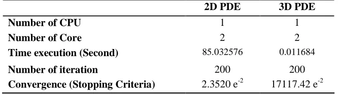
Table 1: Time, Convergence and Number of Iteration for Sequence Algorithm
2D PDE 3D PDE
Number of CPU 1 1
Number of Core 2 2
Time execution (Second) 85.032576 0.011684
Number of iteration 200 200
Convergence (Stopping Criteria) 2.3520 e-2 17117.42 e-2
Table 1 shows that the executive time, convergence and number of iteration for both the 2D and 3D parabolic type PDE with sequential algorithm in solving the mathematical model. The table shows that the executive time for 3D visualisation is much faster than 2D visualisation which uses 1 CPU with 2 cores. Besides, the convergence of 3D visualisation is more than 2D visualisation but the number of iterations performed by both of them is the same.
After running the parallel computing based on 8 numbers of CPU with 16 Cores, the parallel performance will be analysed from the aspect of time execution, speedup, efficiency, effectiveness and temporal performance. The following outcomes show that the increasing number of cores comes with the increased performances in terms of time execution, speedup, efficiency, effectiveness and temporal performance.
B. Multi-Core Parallel programming analysis
The Impact of Number of Cores
The execution time for both 2D and 3D PDEs increases when the number of cores increases. Based of table 2, the speedup also increases when the numbers of cores increases for both the 2D and 3D PDEs but the 3D PDE performs better than the 2D using 16 cores. Actually the real graph of speedup against the number of core is not a straight line in figure 4. It is due to the effect of the communication between the processors. Since the number of cores (16 cores) is limited, the straight lines are not obtained in this study. Besides, the distributed memory hierarchy causes the reduction of the time consuming access to a cluster of workstations.
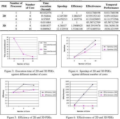
Table 2: Time execution, speedup, efficiency, effectiveness, and temporal performances against different number of cores.
PDE
Number of
Processor Number
of Core
Time execution
(Second)
Speedup Efficiency Effectiveness Temporal
Performance
1 2 85.032576 1 1 0.011760198 0.011760198
4 8 19.56846 4.345389 1.086347 0.555152142 0.051102641
2D
8 16 8.97895 9.470213 1.183776 0.131839093 0.111371596
1 2 0.011684 1 1 85.58712769 85.58712769
4 8 0.001837 6.36037 1.5900925 865.5919978 544.3658138
3D
8 16 0.000963 12.132918 1.5166148 1574.885514 1038.421599
0 10 20 30 40 50 60 70 80 90
2 8 16
Num be r of Core
T
im
e
e
x
e
c
u
ti
o
n
/S
e
c
o
n
d
Time execution/Second (3D) Time execution/Second (2D)
0 2 4 6 8 10 12 14
2 8 16
Num ber of Core
S
p
e
e
d
u
p
Speedup (3D) Speedup (2D)
0 0.2 0.4 0.6 0.8 1 1.2 1.4 1.6 1.8
2 8 16
Num ber of Core
E
ff
ic
ie
n
c
y
Efficiency (3D) Efficiency (2D)
0 200 400 600 800 1000 1200 1400 1600 1800
2 8 16
Num ber of Core
E
ff
e
c
ti
v
e
n
e
s
s
Eff ectiveness (3D) Eff ectiveness (2D) Figure 3: Execution time of 2D and 3D PDEs
against different number of cores
Figure 4: Speedup of 2D and 3D PDEs against different number of cores
Figure 5: Efficiency of 2D and 3D PDEs against different number of cores
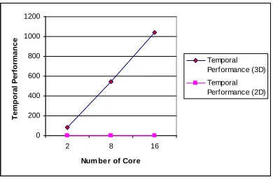
0 200 400 600 800 1000 1200
2 8 16
Num be r of Core
T
e
m
p
o
ra
l
P
e
rf
o
rm
a
n
c
e
Temporal Performance (3D) Temporal Performance (2D)
Figure 5 shows that the efficiency of 3D PDE decreases when we used above 8 cores due to the involvedness of communication. On the other hand, with the 2D PDE, efficiency increases when the numbers of cores increases. The factors that cause the decrease of efficiency are, the imbalance workload, which are distributed among the different cores. The idle time, time start-up and waiting time of all the cores to complete the computations are also the reasons of such efficiency reduction.
Table 2 shows that the effectiveness of 2D PDE decreases when it is used above 8 cores because of the communications and the idle time, time start-up and waiting time of all the cores to complete the computations but the 3D PDE increases remarkably when the number of cores increases. The achievement of result for the increasing effectiveness is based on the increase of the speedup. Moreover the effectiveness of the graph increases when the number of cores is added. A straight line has been formed for the 3D graph due to the communication of the 16 cores where 2D has not provided a straight line in figure 6 due to the same problem discussed above.
Figure 7 shows that the temporal performance increases for both 2D and 3D PDE when the number of cores increases. The graph shows a straight line due to the decreasing of execution time exceedingly in respect of the increasing number of cores.
As summarised in this study, the analysis shows that the performance of the parallel algorithm on multi-core parallel atmosphere is improved by increasing the number of cores from the aspect of speedup, efficiency, effectiveness and temporal performance. Multi-core parallel computing system becomes more famous since these computers provide many order of magnitude raw computing power than the traditional supercomputers at much lower cost. Multi-core parallel computers are now commercially available. They open up new borders in the application of computers, by which many unsolvable (previously) problems can be solved effectively.
The results of the analysis for the performance measurements have proved that multi-core parallel algorithms are considerably better than the sequential algorithms and that 3D PDE performs better than 2D PDE in the visualisation of brain tumour on multi-core parallel atmosphere in terms of speedup, efficiency, effectiveness and temporal performance. The Red-Black Gauss Seidel is found to be suitable for parallel implementation efficiently (Malik Silva, 2003). Besides, the communication of cores and computing times ceaselessly affect the results of speedup, efficiency, effectiveness and temporal performance. The computing of 2D
and 3D parabolic equation of brain tumour growth is well suited by the use of using multi-core parallel computing system because it involved a large space of matrix algorithm.
6. CONCLUSION
The key purpose of this study is to evaluate the performances of multi-core parallel computing system and to compare all the aspects of 2D and 3D partial differential equation in solving the grand challenge of brain tumour visualisation problem. Regarding the growth of brain tumours, a 2D and 3D parabolic model has been chosen to solve this problem by using standard finite difference method.
The explicit method used to solve the evolution equation in this study is the numerical finite difference method. From this study it is proved that the 3D parabolic type PDE performs better than the 2D parabolic type PDE to visualise brain tumour on multi-core parallel atmosphere. Our future comparative study may involve a 3D parabolic type PDE with the other convergent and unconditional stability consisting numerical schemes such as AGE (Alternating Group Explicit) and IADE (Iterative Alternating Decomposition Explicit). As for future research, we aspire to find solutions to improve the speed and performance of the multi-core parallel computing systems, with the increased number of cores to solve the mathematical model.
Acknowledgement
This research is supported in part by the Ministry of Science, Technology and Innovation Malaysia through e-Science funding (Grant No: 78075) and the authors are grateful to Ibnu Sina Institute, University Technology Malaysia for the excellent support to this research.
7. REFERENCES
[1] Deuflhard, P., Seebass, M., Stalling, D., Beck, R & Hege, H. C. 1997, ‘Hyperthermia Treatment Planning in Clinical Cancer Therapy: Modelling, Simulation, and Visualization’, Preprint SC 97-26. Plenary keynote talk, 15th IMACS World Congress 1997 on Scientific Computation, Modelling and Applied Mathematics. In Achim Sydow (ed.), Computational Physics, Chemistry and Biology. Wissenschaft und Technik Verlag, vol. 3, pp. 9-17.
[2] Jianhua Xuan, Isabell A. Sesterhenn, Wendelin S. Hayes, Yue J. Wang, Tulay Adali, Yukako Yagi, Matthew, T. Freedman & Seong K. Mun 1997, ‘Surface reconstruction and visualization of the surgical prostate model’, Proceedings of SPIE, vol. 3031, no. 50.
[3] Lang, J., Erdmann, B. & Seebass, M. 1999, ‘Impact of nonlinear heat transfer on temperature control in regional hyperthermia’, IEEE Transactions on Biomedical Engineering, vol. 46, no. 9, pp. 1129-1138.
[4] Norma Alias, Mohd Ikhwan Safa bin Masseri, Md. Rajibul Islam & Siti Nurhidayah Khalid 2009a, ‘The Visualization of Three Dimensional Brain Tumors’ Growth on Distributed Parallel Computer Systems’, Journal of Applied Sciences. Asian Network for Scientific Information (ANSINET), vol. 9, no. 3, pp. 505-512.
[6] Hogea, Cosmina S., Murray, Bruce T. & Sethian, James A. 2006, ‘Simulating complex tumor dynamics from avascular to vascular growth using a general level-set method’, J. Math. Biol. vol. 53, no. 1, pp. 86-134.
[7] Preziosi, L. 2004, ‘Modeling tumor growth and progression’, In A. Buikis, R. Ciegis & A.D. Fitt, (Eds.), Progress in Industrial Mathematics at ECMI 2002, Springer, pp. 53-66.
[8] Angelis, E. De. & Preziosi, L. 2000, ‘Advection-Diffusion Models for Solid Tumor Evolution in Vivo and Related Free Boundary Problem’, Mathematical Models and Methods in Applied Sciences, vol. 10, no. 3, pp. 379-407.
[9] Bellomo, N. & Preziosi, L. 2000, ‘Modelling and Mathematical Problems Related to Tumor Evolution and Its Interaction with the Immune System’, Mathematical and Computer Modelling, vol. 32, pp. 413-452.
[10] Ambrosi, D. & Preziosi, L. 2002, ‘On the Closure of Mass Balance Models for Tumor Growth’, Mathematical Models and Methods in Applied Sciences, vol. 12, no. 5, pp. 737-754.
[11] Tan Liang Soon & Ang Keng Cheng 2005, ‘A Numerical Simulation of Avascular Tumor Growth’, Anziam J., vol. 46, no. E, pp. C902-C917.
[12] Alfredo Buttari, Jack Dongarra, Jakub Kurzak, Julien Langou, Piotr Luszczek & Stanimire Tomov 2007, ‘The Impact of Multicore on Math Software’, In B. Kagstrom et al. (Eds.), PARA 2006, LNCS 4699, pp. 1–10.
[13] Malik Silva 2003, ‘Cache Aware Data Laying For The Gauss-Seidel Smoother’, Electronic Transactions on Numerical Analysis, vol. 15, pp. 66-77.
Md. Rajibul Islam received his BCA (Bachelor of Computer Applications) degree from the Indira Gandhi National Open University, New Delhi, India, in 2004 and has just completed his M.Sc degree in Information Technology from the Multimedia University, Melaka, Malaysia. Currently he is working as a Research Assistant at the Ibnu Sina Institute for Fundamental Science Studies, in the Science Faculty of the University Technology Malaysia, Johor. His research interests include High Performance Computing (HPC), Numerical Computation, Pattern Recognition, Image Processing, Computer Vision, and Artificial Intelligence.