Scholarship at UWindsor
Scholarship at UWindsor
Electronic Theses and Dissertations Theses, Dissertations, and Major Papers
2012
Global error reduction in vision-based self-localization using a
Global error reduction in vision-based self-localization using a
topological graph representation
topological graph representation
Karam Shaya University of Windsor
Follow this and additional works at: https://scholar.uwindsor.ca/etd
Recommended Citation Recommended Citation
Shaya, Karam, "Global error reduction in vision-based self-localization using a topological graph representation " (2012). Electronic Theses and Dissertations. 4840.
https://scholar.uwindsor.ca/etd/4840
This online database contains the full-text of PhD dissertations and Masters’ theses of University of Windsor students from 1954 forward. These documents are made available for personal study and research purposes only, in accordance with the Canadian Copyright Act and the Creative Commons license—CC BY-NC-ND (Attribution, Non-Commercial, No Derivative Works). Under this license, works must always be attributed to the copyright holder (original author), cannot be used for any commercial purposes, and may not be altered. Any other use would require the permission of the copyright holder. Students may inquire about withdrawing their dissertation and/or thesis from this database. For additional inquiries, please contact the repository administrator via email
REPRESENTATION
byKARAM SHAYA
A Thesis
Submitted to the Faculty of Graduate Studies
through Electrical and Computer Engineering
in Partial Fulfillment of the Requirements for
the Degree of Master of Applied Science at the
University of Windsor
Windsor, Ontario, Canada
2012
c
REPRESENTATION
byKARAM SHAYA
APPROVED BY:
J. Urbanic
Industrial and Manufacturing Systems Engineering
J. Wu
Electrical and Computer Engineering
X. Chen, Advisor
Electrical and Computer Engineering
S. Erfani, Chair of Defense
Electrical and Computer Engineering
Publication
I. Co-Authorship Declaration
I hereby declare that this thesis incorporates material that is result of joint research, as
follows: This thesis also incorporates the outcome of joint research undertaken in
col-laboration with Aaron Mavrinac and Jose Luis Alarcon Herrera under the supervision of professor Xiang Chen. This collaboration is covered in Chapters 1,3,5, and 6 in the thesis.
In all cases, the key ideas, primary contributions, experimental designs, data analysis, and
interpretation were performed by the author, and the contributions of the co-authors was
primarily through the provision of technical content assessment and proof-reading.
I am aware of the University of Windsor Senate Policy on Authorship and I certify that
I have properly acknowledged the contribution of other researchers to my thesis, and have
obtained written permission from each of the co-author(s) to include the above material(s)
in my thesis.
I certify that, with the above qualification, this thesis, and the research to which it refers, is the product of my own work.
II. Declaration of Previous Publication
This thesis includes one original paper that has been previously published/submitted for publication in peer reviewed journals, as follows:
Thesis chapter Publication title/full citation Publication status
Chapters 1,3,5, and 6 K. Shaya, A. Mavrinac, J. L. A. Herrera,
and X. Chen, “A Self-Localization
Sys-tem with Global Error Reduction and
On-line Map-Building Capabilities,” In Pro-ceedings of the International Conference on Intelligent Robotics and Applications (2012), to be published.
Accepted for publication
I certify that I have obtained a written permission from the copyright owner(s) to include
the above published material(s) in my thesis. I certify that the above material describes work completed during my registration as graduate student at the University of Windsor.
I declare that, to the best of my knowledge, my thesis does not infringe upon anyone’s
copyright nor violate any proprietary rights and that any ideas, techniques, quotations, or
any other material from the work of other people included in my thesis, published or
oth-erwise, are fully acknowledged in accordance with the standard referencing practices.
Fur-thermore, to the extent that I have included copyrighted material that surpasses the bounds
of fair dealing within the meaning of the Canada Copyright Act, I certify that I have
ob-tained a written permission from the copyright owner(s) to include such material(s) in my
thesis. I declare that this is a true copy of my thesis, including any final revisions, as ap-proved by my thesis committee and the Graduate Studies office, and that this thesis has not
A single-sensor self-localization system which uses a monocular camera and a set of
artifi-cial landmarks is presented herein. The system represents the surrounding environment as
a topological map (or graph) where each node corresponds to a marker (i.e., artificial
land-mark) and each edge corresponds to the existence of a relative pose between two markers.
The edges are weighted based on an error metric (related to pose uncertainty) and a
short-est path algorithm is applied to the map to compute the path corresponding to the least aggregate error. This path is used to localize the camera with respect to a global
coordi-nate system whose origin lies on an arbitrary reference marker (i.e., the destination node of
the path). Experimental results demonstrate the performance of the system in reducing the
global error associated with large-scale localization.
This work is dedicated to my parents, Adel Shaya and Khalida Sakee.
First, I would like to express my sincere gratitude towards my thesis advisor, Dr. Xiang
Chen, for his encouragement, guidance, patience, and above all, faith in my abilities to
complete my research work. Special thanks to my committee members, Dr. Jonathan
Wu and Dr. Jill Urbanic, for enriching the quality of my work through their invaluable
suggestions and insight. I want to thank my colleagues in the Advanced Control Systems
Laboratory, especially those in the computer vision group: Aaron Mavrinac, Jose Alarcon, Davor Srsen, and Durga Rajan. Their support and understanding during my moments of
doubt has meant more to me than I could express. Finally, I am forever indebted to my
loving family for everything they have done for me throughout my life.
Declaration of Co-Authorship / Previous Publication iii
Abstract v
Dedication vi
Acknowledgements vii
List of Figures xii
List of Tables xv
1 Introduction 1
1.1 Single-Sensor Vs. Multi-Sensor Systems . . . 1
1.2 The Camera As a Sensor in Self-Localization Systems . . . 2
1.3 Local and Global Error . . . 2
1.4 Existing Systems That Utilize Graphical Representations in Pose Estima-tion ApplicaEstima-tions . . . 3
1.5 Single-Sensor, Vision-Based Self-Localization Systems . . . 3
1.6 Main Contribution . . . 5
2 Theoretical Foundation 6 2.1 Image Formation . . . 6
2.2 The Pinhole Camera Model . . . 9
2.2.1 3D Euclidean Transformation . . . 10
2.2.2 3D-2D Projection . . . 10
2.2.3 2D-2D Transformation . . . 12
2.2.4 Combining the Transformations . . . 13
2.3 Camera Calibration . . . 13
2.4 Pose . . . 16
2.4.1 Pose Composition . . . 16
2.4.2 Relative Pose Calculation . . . 17
2.5 Shortest Path Algorithm . . . 18
3 Proposed Solution 19 3.1 Preliminaries . . . 19
3.1.1 Marker Graph . . . 19
3.1.2 Localization Graph . . . 20
3.2 Global Localization . . . 20
3.2.1 Assumptions . . . 20
3.2.2 Problem Definition . . . 20
3.2.3 Self-Localization Method . . . 21
3.2.4 Self-Localization Algorithm . . . 23
4 Implementation 25 4.1 Marker Design . . . 25
4.1.1 Outer Border . . . 29
4.1.2 Inner Code . . . 30
4.2 Software Implementation . . . 31
4.2.1 Internal Camera Calibration . . . 31
4.2.2 HDevelop Program . . . 32
4.2.3 Python Program . . . 37
4.3 Hardware Implementation . . . 40
5 Experiments 41 5.1 Purpose . . . 41
5.2 Experimental Setup . . . 41
5.3 Error Metrics . . . 42
5.3.1 Reprojection Error Metric . . . 42
5.3.3 Error Ellipse Volume Metric . . . 43
5.3.4 Perpendicular Distance Metric . . . 44
5.4 Experiment to Compare the Error Metrics . . . 44
5.4.1 Procedure . . . 45
5.4.2 Results . . . 47
5.4.3 Analysis . . . 49
5.5 Experiment to Examine the Effect of Implementing an Error Metric on the Global Scale . . . 50
5.5.1 Procedure . . . 50
5.5.2 Results . . . 53
5.5.3 Analysis . . . 55
5.5.4 Limitations . . . 55
6 Conclusion 56 6.1 Summary of Contributions . . . 56
6.2 Future Work . . . 56
A Glossary of Terms 58 B HDevelop Program Source Code 61 B.1 Main Program . . . 61
B.2 Function:get quad corners . . . 71
B.3 Function:is quad inside . . . 75
B.4 Function:calc cross ratio . . . 77
C Python Program Source Code 78 D Data Tables 88 D.1 Ground Truth Error Vs. Error Metrics . . . 88
D.2 Ground Truth Error Vs. Aggregate Errors of Perpendicular Distance Func-tions . . . 90
E.2 Permission to Use Dr. Boufama’s Lecture Notes . . . 94
References 95
2.1 Illustration of the process of image formation. . . 7
2.2 Illustration of the pinhole camera model. . . 9
2.3 Perspective projection of a 3D pointP to a 2D pointpon an image plane. . 11
2.4 An example calibration pattern. . . 14
2.5 Relative pose calculation: The camera can calculate the relative pose trans-formation between multiple markers by capturing them concurrently in its FOV. . . 17
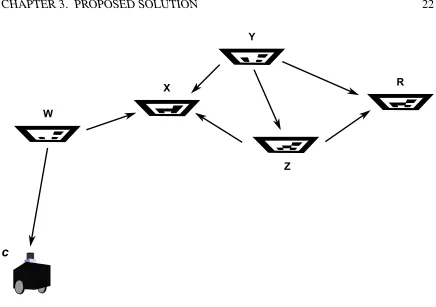
3.1 Camera pose estimation: Arrows indicate the direct pose estimate of one object (camera or marker) with respect to another, where the pose of the object on the arrow’s tail is given with respect to that on the arrow’s head. . 22
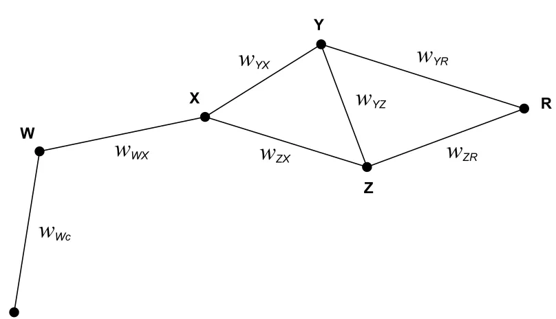
3.2 Localization graph for system in Figure 3.1: Edge weights represent pose estimation uncertainty values. . . 23
4.1 ARToolKit (ATK) marker design . . . 26
4.2 Hoffman marker system (HOM) marker design . . . 26
4.3 Institut Graphische Datenverarbeitung (IGD) marker design . . . 27
4.4 Siemens Corporate Research (SCR) marker design . . . 27
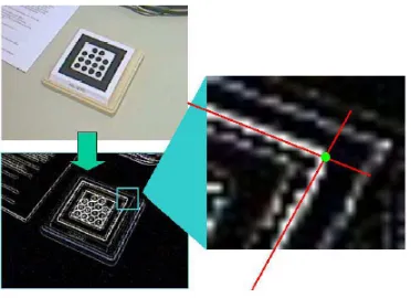
4.5 Finding the ground truth of the marker corners using edge detection, least-squares fitting, and intersection calculation. . . 28
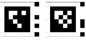
4.6 Marker design: Two examples of the markers used in the implementation of the localization system. . . 29
4.7 Cross-ratio constraint: The diagonal corners of the inner and outer edges (labeled A, B, C, and D) of the border are used to calculate the cross-ratio. . 30
4.8 Marker code: The coded area of the marker lies within the border and is divided into nine cells. . . 31
4.9 HALCON’s calibration plates: Sample images from HALCON’s image
database illustrating the process of internal camera calibration through the
use of calibration plates. . . 32
4.10 Current frame capture. . . 33
4.11 Contrasted frame. . . 33
4.12 Refined image of the marker code displayed without perspective distortion. 34 4.13 Sampled regions of the marker code (one per cell). . . 34
4.14 Displaying the coordinate axes of the marker after its true pose is found. . . 35
4.15 Positional relationship between a point and a convex polygon: Considering the polygon as a path to determine whether a point lies within it. . . 37
4.16 Output of the Python program. . . 40
5.1 Visual description of the reprojection error (the pixel distance between the arrows). . . 42
5.2 Progressively blurrier image captures of a marker. Note how the edges are less distinctively defined in the blurrier captures. . . 43
5.3 An error ellipse representing the positional uncertainty of the marker origin. 44 5.4 The perpendicular distance between the camera and a marker. . . 45
5.5 An illustration of the different positions that the camera is placed and local-ization results are recorded for the local scale experiment. The grid starts at a distance of 1.116mfrom the marker in the negativezdirection, 0.313 min theydirection and is centered atx= 0m. The dimensions of the grid are2.508×0.456m with the spacing between the dots along thexandy directions being 0.228m. . . 46
5.6 Graph of ground truth error vs. the reprojection error metric. . . 47
5.7 Graph of the ground truth error vs. the blur metric. . . 47
5.8 Graph of the ground truth error vs. the error ellipse volume metric. . . 48
5.10 An illustration of the different positions that the camera is placed and
lo-calization results are recorded for the global scale experiment. The grid
starts at a distance of 0.888mfrom the reference marker in the negativez
direction, 0.313m in the ydirection and with its right edge at x = 0m. The dimensions of the grid are2.508×0.456mwith the spacing between the dots along thexandydirections being 0.228m. . . 51 5.11 Experimental map: (a) arrangement of markers in the environment, (b)
topological representation of the map. . . 52
5.12 Three image captures of the marker configuration and experiment setup. . . 52
5.13 Graph of ground truth error vs. the aggregate error based on the linear
function (f(d) =d) of the perpendicular distance metric. . . 53 5.14 Graph of ground truth error vs. the aggregate error based on the quadratic
function (f(d) =d2) of the perpendicular distance metric. . . . 53 5.15 Graph of ground truth error vs. the aggregate error based on the exponential
function (f(d) = 3d−1) of the perpendicular distance metric. . . 54 5.16 Graph of ground truth error vs. the aggregate error based on the exponential
D.1 Raw data for the Ground Truth Error Vs. Error Metric figures. . . 88
D.2 Raw data for the Ground Truth Error Vs. Aggregate Error figures. . . 90
Introduction
With the growing demand for autonomous robots in industrial, medical, domestic, and other
domains, a large portion of research in the robotics industry has been geared toward the development and improvement of self-localization systems (i.e., systems that can estimate
their own pose within an environment through the use of sensors).
1.1
Single-Sensor Vs. Multi-Sensor Systems
For the purposes of this work, existing self-localization systems in the literature will be
divided into two categories: those that obtain their data from multiple sensors (e.g., [14],
[3], [8]) and those that obtain them from a single sensor (e.g., [20], [30], [32]). The former type of system takes a sensor fusion approach. One major advantage of sensor fusion is the
availability of multiple sources of data, through which the robot may verify the readings of
its individual sensors and reduce the overall error of its pose estimates. The disadvantages
of using multiple sensors are added complexity (in the localization1algorithm and hardware
design), larger form factor, and increased cost. Conversely, systems that use single-sensors
tend to be simpler, smaller, and less expensive; however, they do not have the redundancy
and fusion of multiple independent sensor measurements and must therefore use internal
methods to reduce estimation error. The focus of this work is on reducing the estimation
error of a single sensor localization system. A camera will be used as the sensor.
1The terms “self-localization” and “localization” refer to the same concept and will be used
interchange-ably throughout the thesis
1.2
The Camera As a Sensor in Self-Localization Systems
Compared to the sensing modalities used in other solutions (e.g., odometry, sonar, and laser), two-dimensional camera images provide a robot’s localization algorithm with more
data about the environment [17]. They can be used by a localization system to detect,
identify, and estimate the pose of objects in a scene with respect to the camera’s coordinate
system. The pose of the object can then be inverted to estimate the camera’s pose with
respect to the object’s coordinate system. Self-localization is achieved when the object’s
coordinate system is also the global coordinate system of the environment.
However, when the object falls outside the camera’s sensing range, its pose cannot be
found directly. Therefore, a map must be built to represent its surrounding environment
such that when the object is outside the camera’s FOV (field of view), there is a path back to the object through the map.
1.3
Local and Global Error
The nature of the map-building process of vision-based self-localization yields two
par-ticular types of pose estimation errors: local error, which originates from error and noise in image capture and affects pose estimations made with respect to local coordinate
sys-tems in the image, andglobal error, which arises from the accumulation of local error and affects pose estimations made with respect to a global coordinate system that may not
nec-essarily be in the image. Due to the influence local error has on global error, reducing the
former would result in a reduction of the latter. Local error reduction is implemented in the
proposed system herein through the use of markers (i.e., artificial landmarks2) that can be
accurately detected and discerned in a two-dimensional image [12], [7], [19].
With regards to the general goal of this work, however, a different perspective is taken:
while reducing local error will cause a reduction in the global error, a more direct approach
to reducing global error is by representing the surrounding environment as a topological
map/graph whose edge weights reflect the effects of local error.
2Landmarks are objects with distinct features that make them relatively easy to separate from their
1.4
Existing Systems That Utilize Graphical
Representa-tions in Pose Estimation ApplicaRepresenta-tions
Graphical representation in similar pose estimation problems has previously been applied
to such areas as multiview registration of 3D scenes and large-scale external calibration of
camera networks. Sharp et al. [28] present a graphical approach to modeling neighbouring
(i.e., overlapping) views in a network of range scanners (laser-based sensors). They apply
an optimization to the graph to reduce the global error associated with multiview
registra-tion of 3D scenes. In the area of multi-camera calibraregistra-tion (where the external parameters
include the relative poses between the cameras), Brand et al. [6] use the graphical approach
to apply constraints on the viable positions of the cameras with respect to each other. This, like the system by Sharp et al. also uses neighbouring views to determine relative poses
between the cameras.
There also exist a number of multi-sensor self-localization systems that use the
graph-ical representation. The system introduced by Thrun and Montemerlo [29], called Graph-SLAM (where SLAM is an acronym forSimultaneous Localization and Mapping), uses a robot called Segbot that utilizes a scanning laser, an inertial measurement unit, and a GPS
as its sensors. Each edge of its graph represents a nonlinear constraint that is weighted
based on the uncertainty associated with the sensor measurements and the motion model.
The map-building for this particular system is done offline. A similar system called Graph-ical SLAM, designed specifically for outdoor applications, is proposed by Folkesson and Christensen [13]. Like the Segbot, it uses a scanning laser and an inertial measurement unit
as its sensors and like the system by Thrun and Montemerlo, it represents the environment
as a topological graph with nonlinear constraints between detected features.
To the best of the author’s knowledge, a single-sensor vision-based self-localization
system utilizing the topological graph representation has not been presented in literature.
1.5
Single-Sensor, Vision-Based Self-Localization Systems
The following systems perform localization solely through the use of a vision-based sensor
(i.e., a camera). Note that purely vision-based localization systems are not very common
re-ality, where large scale localization is not required in many cases. These systems do not
implement a graphical representation of the environment but are presented to introduce the
reader to some current vision-based localization systems in literature.
An Extended Marker-Based Tracking System for Augmented Reality
Jun et al. [15] propose a ceiling-based marker tracking system. There are two planar marker
systems which are explained in detail in this paper: ARToolkitPlus and ARTag. These sys-tems take the captured images of the markers as input and then output their pose with
respect to the camera which captured them. ARToolkitPlus uses a simple grayscale
inten-sity threshold to extract the fiducial marker from the image; then it identifies the marker
based on its pattern; and finally, it calculates the homography using the square black
bor-der which surrounds the marker pattern. However, with the use of a global threshold, the
output can be affected by abnormal lighting, even if it only affects a single image. In
con-trast, the ARTag system completes these tasks by usingdifferentialintensity thresholds to extract edges from the marker. ARTag identifies each marker by its extracted edge pattern.
It uses the corners of the quadrilaterals in the pattern (formed by the edges) to calculate each marker’s homography.
The idea of using multiple markers stems from the need to extend the range of the
global coordinate system. Hence, transformations of the local coordinate systems of each
marker to the global coordinate system are required to be found.
Real-Time Camera Pose Estimation for Augmented Reality System Using a Square
Marker
Most current augmented reality systems use markers in the scene to estimate the pose of
the device with respect to the global coordinate system. However, when these markers are
blocked by obstacles or they fall out of the view of the camera, the pose estimation cannot
be calculated with sufficient accuracy, if at all. An example of such a system is ARToolkit. Lee et al. [18] present a method to handle the problems caused by occlusions. In the
captured image, the features are detected using the Shi-Tomasi corner detector. Next, these
features are tracked using a Lukas-Kanade Tracker (LKT), which is appropriate for this
application due to its ability to perform in real-time. However, the trade-off for the LKT’s
vision. When the marker falls out of range of the LKT, the features must be re-detected and
the tracking must be restarted.
A Six-DOF Motion Tracking System for Markered Environment
Yang et al. [31] describe a method of camera pose estimation using a non-traditional
marker-based system. Infrared LEDs are placed on the ceiling as markers in a
predeter-mined pattern. An offline process is undertaken to determine the 3D coordinates of each
LED with respect to a common world coordinate system. An infrared filter is placed on
the camera to reduce the effects of illumination changes by filtering out most of the visible
light spectrum.
During the offline process, a set of images are taken from multiple points of view, their
features are extracted, labeled, and matched. Then, an incremental iterative optimization
method is applied to obtain each LED’s 3D coordinate.
During the online process, the information obtained through the offline process is used
to estimate the pose of the camera: 2D feature points are extracted from each frame in the
live video and matched with their corresponding 3D coordinates of the LEDs.
1.6
Main Contribution
The main contribution of the proposed system is the application of established topological
map representation methods to reduce global error in single-sensor vision-based
localiza-tion systems.
By applying a shortest path algorithm, the map can be optimized to yield the paths of
minimum global error (i.e., accumulated local error) from the camera to the global
coordi-nate system. Furthermore, this system will provide the potential for online map-building in
implemented systems, precluding the need for preliminary training.
The topological graph representations of the environment are as follows: the markers will represent the vertices, the existence of a relative pose between two markers will be
represented by an edge, and the edge weights will be based on an appropriately derived
Theoretical Foundation
Information obtained from a camera comes in the form of 2D images. In applications
in-volving localization in a 3D environment, 2D images can be used to indirectly obtain 3D information. This can be done by using multiple cameras to find point correspondences
between multiple views and performing triangulation on the points. Another, more
eco-nomical, method is through the use of a single camera and a priori data about targets (i.e.,
markers) in the image – as in the proposed system herein. This chapter will explain the
theoretical background regarding the extraction of 3D information from 2D images1:
2.1
Image Formation
When a 3D representation of a scene is reduced to 2 dimensions, the result is called an
image. More specifically, an image captured by a camera (either CMOS2or CCD3 type) is
the result of a 3D geometric transformation, which takes 3D information and describes it
in a 2D framework.
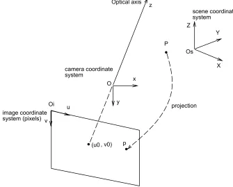
A coordinate system having an originO, called thecenter of projection, and three axes,
Ox, Oy, Oz, will be used to represent the reference frame (i.e., coordinate system) of the camera; it is illustrated in Figure 2.1. It can be noted that theOxandOy axes are parallel to 1The information of Sections 2.1, 2.2, and 2.3 is based on the lecture notes of 03-60-551 (Visual
Process-ing), prepared by Dr. Boubakeur Boufama – a professor in the School of Computer Science at the University of Windsor. The figures used are also credited to the same lecture notes by Dr. Boufama.
2Complementary Metal-Oxide-Semiconductor 3Charge-Couple Device
the image plane and are correspondent to the row and column directions, respectively. Oz, called theoptical axis, is perpendicular to the image plane.
u
x
y
Oi projection
z
P
p v
Optical axis
(u0 , v0) image coordinate
system (pixels)
camera coordinate system
Z
X Y
Os
scene coordinate system
O
Figure 2.1: Illustration of the process of image formation.
Three geometric transformations, applied in sequential order, are required to express 3D scene points in 2D image coordinates (i.e., pixels):
1. A 3D Euclidean transformation: A transformation is applied to the 3D points, defined in the scene coordinate system, such that they are expressed in the camera coordinate
system. Six parameters are involved in this transformation, corresponding to the
translation and rotation operations, each with respect to the three axes.
2. A 3D-2D projection: The 3D points in the camera coordinate system are projected
onto the image plane and are now referred to asnormalized coordinates.
3. A 2D-2D transformation: An affine transformation is applied to the normalized
coor-dinates to express the 2D point in pixel coorcoor-dinates in the image plane. It is expressed
A =
αu −αucot θ u0
0 αvsin θ v0
0 0 1
(2.1)
where,
• αu andαv are scale factors along theOxandOy directions, respectively.
– αu =−f ku andαv =−f kv.
– f is the distance (usually in mm) between O and the image plane, called the
focal length.
– ku and kv are the number of pixels per mm along theOx and Oy directions, respectively.
• u0andv0are the pixel coordinates of the center of the image, which is defined as the intersection of the optical axis and the image plane.
• θ is the angle between theuandv axes of the image. Due to some errors that arise during the manufacturing process of the camera, this angle may not be exactlyπ/2. However, in the modern cameras, it can be assumed that it is equal toπ/2because the error is so small. Therefore, equation (2.1) may be expressed as shown in equation
(2.2).
A=
αu −αu u0
0 αv v0
0 0 1
(2.2)
Combining the three geometric transformations above, the following matrixMis obtained:
M =AID (2.3)
where,
• Ais the 2D-2D transformation,
• andDis the 3D Euclidean transformation.
2.2
The Pinhole Camera Model
There are a number of ways to approximately model the geometry of a camera; three pop-ular ones are the pinhole model, the orthographic model, and the weak perspective model.
The most widely used approximation for cameras, however, is the pinhole model. This is
the model on which the proposed system will be based. In this model, the 3D-2D projection
of a point a 3D pointP to a 2D pointp(on an image plane) is a pure perspective projection throughO (as in Figure 2.2). With this information, the geometric transformations will be explained in the context of the pinhole camera model.
u
x
y Oi
projection z
P
p v
Optical axis
(u0 , v0) image coordinate
system (pixels)
camera coordinate system
Z
X Y
Os
scene coordinate system
O
2.2.1
3D Euclidean Transformation
Assume that points P = (X, Y, Z) and P0 = (X0, Y0, Z0) represent the same physical point, where P is defined in the scene coordinate system, and P0 is defined in the camera coordinate system. The relationship betweenP andP0is given in equation (2.4), where the matrix ofrij entries represents a rotation and the vector with entriestx, ty,andtzrepresents a translation. Both operations are being applied to the pointP.
X0 Y0 Z0 =
r11 r12 r13
r21 r22 r23
r31 r32 r33 X Y Z + tx ty tz (2.4)
Using homogeneous coordinates, equation (2.4) can be expressed as
X0 Y0 Z0 1 =
r11 r12 r13 tx
r21 r22 r23 ty
r31 r32 r33 tz 0 0 0 1
X Y Z 1 (2.5)
or more conveniently as
P0 =DP (2.6)
where,
• Dis a4×4matrix that represents a rigid 3D displacement.
• P andP0 are the homogeneous coordinates expressed with respect to the scene and camera coordinate systems, respectively.
2.2.2
3D-2D Projection
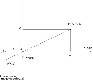
Figure 2.3 illustrates how a 3D point, P(X, Y, Z) is projected onto an image plane to become a 2D point,p(x, y).
Note that the focal lengthf is also represented in the image.
P
O
p
Image plane
(X, Y, Z)
(x, y) Z f Z−axis (0, 0) (Image coordinate) X−axis X
Figure 2.3: Perspective projection of a 3D pointP to a 2D pointpon an image plane.
Z f =
X
x ⇒x=f X
Z (2.7)
Z f =
Y
y ⇒y=f Y
Z (2.8)
These equations can be expressed in matrix form as in equation (2.9), where f = 1 is assumed. x y 1 =λ
1 0 0 0
0 1 0 0
0 0 1 0
X Y Z 1 (2.9)
which can be compacted to the following:
where,
• I is a3×4matrix that represents perspective projection.
• λis a scale factor.
Therefore, obtaining a projected point pof a 3D pointP, expressed in the scene coor-dinate system would require the operation
p=λIDP (2.11)
whereDaltersP such that it is expressed in the camera coordinate system andI applies a perspective projection to express its 2D projection on the plane.
2.2.3
2D-2D Transformation
To express P in pixel coordinates, two further operations must be performed: a scaling and a translation. This is done by applying the matrixA, defined in Section 2.1. Although the scaling changes the units to pixels, the translation must be applied so that the origin of
the coordinate system is moved to the upper-left corner of the image plane4. In equation
form, the pixel coordinates(u, v)(whereuandvare the column and row indices of a pixel, respectively) corresponding to the projection ofP are given in equations (2.12) and (2.13).
u=αux+u0 (2.12)
v =αvy+v0 (2.13)
The following equations expresses these in matrix form:
u v 1 =
αu 0 u0
0 αv v0
0 0 1
x y 1 (2.14)
2.2.4
Combining the Transformations
Recall from equation (2.3) thatM = AIDis the matrix representing the three combined transformations. After performing matrix multiplication,M is expressed in the form of
M =
αur11+u0r31 αur12+u0r32 αur13+u0r33 αutx+u0tz
αvr21+v0r31 αvr22+v0r32 αvr23+v0r33 αvty +v0tz
r31 r32 r33 tz
(2.15)
However, for simplicity, it will be represented as
M =
m11 m12 m13 m14
m21 m22 m23 m24
m31 m32 m33 m34
(2.16)
Hence, the pixel coordinatespi = (ui, vi)of the projected 3D pointPi = (Xi, Yi, Zi)can be found by the following equation:
ui vi 1 =λ
m11 m12 m13 m14
m21 m22 m23 m24
m31 m32 m33 m34 Xi Yi Zi 1 (2.17)
which, in equation form, becomes
ui =
m11Xi+m12Yi+m13Zi+m14
m31Xi+m32Yi+m33Zi+m34
(2.18)
vi =
m21Xi+m22Yi+m23Zi+m24
m31Xi+m32Yi+m33Zi+m34
(2.19)
2.3
Camera Calibration
Camera calibration is a process by which a camera’s internal/intrinsic (i.e., focal length,
pixel cell dimensions, optical center, etc.) and external/extrinsic (i.e., pose of the camera
estimation of the projection matrixM.
InM, there are a total of 12 unknowns to be estimated. To solve the unknowns, corre-sponding pixel and 3D coordinates of the same points in a scene can be used as constraints.
Pixel coordinates of points of interest can be retrieved from a captured image after they are
detected by their features (either manually or automatically). The corresponding 3D
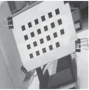
coor-dinates of the same points must be known a priori through measurement (e.g., using laser or accurate ruler). Calibration patterns, such as the one in Figure 2.4, are used because the
3D coordinates of their patterns with respect to the scene coordinate system can be easily
obtained and their features can be accurately detected in an image. With calibration plates,
the scene coordinate system can be chosen to lie on their surface so that the 3D coordinates
are essentially reduced to 2 dimensions, further simplifying the process.
Figure 2.4: An example calibration pattern.
The calibration process begins by putting a calibration pattern in front of the camera and
adjusting the camera (i.e., focus) until a clear picture of the pattern can be seen. From this
position, an image is taken. The points of interest in the image are extracted and matched
with their corresponding 3D points. The 2D and 3D points are input into a calibration software to estimateM.
EstimatingM
Assuming the availability of 2D-3D point correspondences, (ui, vi) and (Xi, Yi, Zi) in equations (2.18) and (2.19) are known. Rearranging these equations results in the
ui −
m11Xi+m12Yi+m13Zi+m14
m31Xi+m32Yi+m33Zi+m34
= 0 (2.20)
vi−
m21Xi+m22Yi+m23Zi+m24
m31Xi+m32Yi+m33Zi+m34
= 0 (2.21)
Note that these equations are non-linear. The equations are linearized by multiplying both sides of the equations by the denominators:
ui(m31Xi+m32Yi+m33Zi+m34)−(m11Xi+m12Yi+m13Zi+m14) = 0 (2.22)
vi(m31Xi+m32Yi+m33Zi+m34)−(m21Xi+m22Yi+m23Zi+m24) = 0 (2.23) Whennpairs of points(Pi, pi),i= 1, . . . , n, are available, equations (2.22) and (2.23) can be written in matrix form as
−X1 −Y1 −Z1 −1 0 0 0 0 u1X1 u1Y1 u1Z1 u1
0 0 0 0 −X1 −Y1 −Z1 −1 v1X1 v1Y1 v1Z1 v1
−X2 −Y2 −Z2 −1 0 0 0 0 u2X2 u2Y2 u2Z2 u2
0 0 0 0 −X2 −Y2 −Z2 −1 v2X2 v2Y2 v2Z2 v2
.. .
−Xn −Yn −Zn −1 0 0 0 0 unXn unYn unZn un
0 0 0 0 −Xn −Yn −Zn −1 vnXn vnYn vnZn vn
m11 m12 m13 m14 m21 m22 m23 m24 m31 m32 m33 m34 = 0 (2.24)
Representing this in a compact form:
AV = 0 (2.25)
• Ais a2n×12measurement matrix.
• V is 12-element vector consisting of unknown elements.
To solve for the 12 entries ofM,nmust be greater than or equal to 6, implying that at least 6 point correspondences are necessary to solve for all entries ofM.
Note that if the internal camera parameters, such as the focus, are not altered during the
course of self-localization, the results do not require recalculation; a single calibration is
sufficient before the online self-localization begins. However, the same does not hold true
for the external parameters, as they are constantly changing as the camera moves.
2.4
Pose
2.4.1
Pose Composition
A posePαβ is a rigid three dimensional Euclidean transformation from the coordinate sys-tem of objectαto the coordinate system of objectβ. This may be referred to as the pose of objectαwith respect to objectβ.
The inverse of posePαβ may be denotedPαβ−1 orPβα. The former notation will be used here to emphasize thatPαβ is the available direct estimate.
Successive pose transformations may be composed into a single pose:
Pαγ(p) = (Pαβ◦Pβγ)(p) = Pβγ(Pαβ(p)) (2.26) Note that a left-composition convention is used to better illuminate the sequence of pose
transformations.
The details of pose inversion and composition vary depending on the representation
used. The reader is directed to any of the numerous texts on Euclidean geometry for a
2.4.2
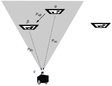
Relative Pose Calculation
Referring to Figure 2.5, the relative pose transformation of a marker α with respect to another markerβ is determined through pose composition to be
Pαβ =Pαc◦Pβc−1 (2.27)
wherePαcand Pβc are the poses ofα andβ with respect to the camerac(assumed to be available). Note that this calculation is made possible by the fact that both markers are in
the camera’s FOV (shaded area in Figure 2.5) at the same time; more specifically, pose
estimates are taken from the same captured camera frame.
β
Pαc
Pβc
c
α
Pαβ
2.5
Shortest Path Algorithm
Shortest path algorithms can be applied to graphs to find the minimum topological path between two nodes. The famous shortest path algorithm by Dijkstra [10] solves the
single-source shortest path problem of undirected graphs with non-negative edge weights. Since
globally localizing a camera involves obtaining its pose with respect to a single source
(i.e., the global coordinate system), Dijkstra’s algorithm is appropriate for computing the
Proposed Solution
3.1
Preliminaries
3.1.1
Marker Graph
Themarker graph(based on thecalibration graphintroduced by Mavrinac et al. [22]) is a method of representing a set of markers as a topological map. It is a weighted, undirected
graphGM = (M, EM,WM), whereMis the set of detected markers in the system,EMis a set of edges, andWM is the set of weights corresponding to the edges inEM. The existence of an edge {α, β} ∈ EM indicates that a relative pose transformation from marker α to markerβ(or vice versa) is available.
Since it is trivial to invert a pose, the availability ofPαβ implies availability ofPβα. The edge weight(wαβ ∈R+)∈ WM is the estimation uncertainty ofPαβ.
A path p = hα, . . . , βiin GM, from nodeα to node β, represents a sequence of pose transformations which may be composed to yieldPαβ. Ifp=hv1, v2, . . . , vni,
P1,n =P1,2◦P2,3◦ · · · ◦Pn−1,n (3.1) wherePi,j is the pose transformation fromvitovj. If anyPi,j is not available,Pi,j =Pj,i−1. The aggregate error associated with this pose is
w1,n = n
X
2
wk−1,k (3.2)
which is the length of pathp.
3.1.2
Localization Graph
Thelocalization graphis essentially a marker graph that includes the cameracas an addi-tional node. It is a weighted, undirected graphGL= (L, EL,WL), whereL =c∪ M, EL is the set of edges between nodesL, and WL is, again, the set of associated edge weights. The localization graph is incrementally updated as the cameracmoves through the envi-ronment. Note thatGL ⊃ GM.
3.2
Global Localization
3.2.1
Assumptions
Internal Calibration and Pose Estimation
It is assumed that there exists some means by which a camera may estimate, from a
sin-gle view, its relative three dimensional pose with respect to a calibration target of known
structure [35], [4]. This normally implies that the camera is internally calibrated.
Marker Constraints
It is assumed that (i) if a markerm ∈ M is connected to an edge, it remains fixed in its position, and (ii) the selected reference node R corresponds to a marker that is available and detectable in the environment.
Map Updates
It is assumed that any operation that updatesGM simultaneously updatesGL, and vice versa.
3.2.2
Problem Definition
The problem of global localization using computer vision is formalized as follows:
Let us further define a set of markers V which are in the camera’s current FOV (e.g., shaded area in Figure 2.5). Then, it can be noted thatPcR may either be obtained directly fromR(whenR ∈ V) or indirectly from another marker v ∈ V (whenR /∈ V), assuming there exists a path inGLfromctoR.
It is additionally desirable to decrease the global error by using the pathpyielding the minimum aggregate error (as defined in (3.2)) for each estimatedPcR.
3.2.3
Self-Localization Method
The method will be explained with the aid of an example. Suppose it is desired to find
the pose of a monocular camera c within an environment consisting of markers M =
{W, X, Y, Z, R}, as shown in Figure 3.1. In this case,Ris selected as the global reference frame, so the problem is to findPcR. As mentioned previously, there are two ways of finding
PcR: either directly throughR (whenR is in the FOV) or indirectly through intermediate markersW, X, Y, Z (whenRis not in the FOV).
As shown in Figure 3.2, the localization graph is connected assuming that the direct
pose estimates in Figure 3.1 are all available. Thus, the camera c can be localized with respect to the common reference frameRusing any of the markers in the map.
The minimum requirement to achieve global localization is that there must exist a path
from the current position ofcto the reference frameRinGL. Additional edges may yield shorter paths (i.e., pose compositions with lower aggregate error). The positioning of the
set of markersMshould be chosen appropriately. Note that there is no disadvantage, aside from additional effort positioning and obtaining pose estimates, to increasing the size of
M.
In this example, direct pose estimates PW c, PW X,PY X, PZX,PY Z, PY R, andPZR are obtained, along with their respective pose uncertainties. The availability of direct pose
estimates is encapsulated in the localization graph of Figure 3.2.
The solution is obtained through composition of the estimated poses, according to (3.1),
where the shortest paths are computed using Dijkstra’s algorithm or similar. As an example,
suppose the shortest path fromctoRinGLishc, W, X, Y, Z, Ri. Then,
W
X
Y
Z
R
c
Figure 3.1: Camera pose estimation: Arrows indicate the direct pose estimate of one object (camera or marker) with respect to another, where the pose of the object on the arrow’s tail is given with respect to that on the arrow’s head.
as per (3.1). The associated aggregate error iswcR =wW c+wW X +wY X +wY Z+wZR.
Map Updating
When there are multiple markers in the FOV, the relative poses between all possible pairs
of markers in the frame are calculated and connecting edges (with associated weights) are
created between them. If in a subsequent frame an edge is re-detected and is found to have
a lower weight than the existing edge, its relative pose transformation and weight overwrite
W
X
Y
Z
R
c
w
Wcw
WXw
ZXw
YXw
ZRw
YRw
YZFigure 3.2: Localization graph for system in Figure 3.1: Edge weights represent pose estimation uncertainty values.
3.2.4
Self-Localization Algorithm
In the formal expression of the algorithm (Algorithm 1), let primed (0) variables represent
Algorithm 1Proposed Self-Localization Algorithm (FindingPcR0 )
1: M ← {R}
2: EM,WM,V ← ∅
3: n←F alse
4: loop
5: Capture frame 6: ifV 6=∅then
7: M ← M ∪ V
8: if|V|>1then
9: for all{vi, vj} ∈ V2
do
10: Pij0 ←Pic0 ◦Pjc0−1
11: Pji0 ←Pij0−1
12: if{vi, vj}∈/ EM then
13: EM ←EM ∪ {vi, vj}
14: wij, wji← ∞
15: WM ← WM ∪wij, wji
16: end if
17: ifcalcw0({vi, vj})< wij then
18: wij, wji←calcw0({vi, vj})
19: Pij ←Pij0
20: Pji←Pji0
21: n←T rue
22: end if
23: end for
24: ifn=T ruethen
25: for all{m∈ M |con(GM, m, R)}do
26: ps ←sp(GM, m, R)
27: PmR←Pps,1,ps,2
28: wmR←wps,1,ps,2
29: fork= 2→ |ps| −1do
30: PmR ←PmR◦Pps,k,ps,k+1
31: wmR←wmR+wps,k,ps,k+1
32: end for
33: end for
34: end if
35: end if
36: ifR ∈ Vthen
37: PcR0 =PRc0−1
38: else if∃ {v∈ V |con(GM, v, R)}then
39: vm←argmin
v∈V
(calcw0({v, c}) +wvR)
40: PcR0 ←Pv0m−1c◦PvmR
41: end if
42: end if
43: n=F alse
Implementation
4.1
Marker Design
Existing Marker Designs in Literature
The survey paper by Zhang et al. [33] provides a comparison of a few marker designs to
give the reader a background of existing marker systems in literature1. These systems are
compared quantitatively and qualitatively in terms of four criteria: usability, efficiency,
accuracy, and reliability. In most marker systems, the square shape is utilized for pose
estimation because it provides four easily detectable point correspondences (corners of the square). The following square-based marker systems were compared:
• ARToolKit (ATK) [16]
• Hoffman marker system (HOM)2
• Institut Graphische Datenverarbeitung (IGD) [1]
• Siemens Corporate Research (SCR) [34]
These four systems were chosen for their availability, expandability, and because they
are suitable to represent other similar marker systems. The design of each marker is
pre-sented as follows:
1The information and figures of the existing marker designs presented in this section are credited to Zhang
et al. [33]
2Developed by C. Hoffmann in 1994 at Siemens AG.
ARToolKit (ATK) (Figure 4.1) The ATK system performs simple template
match-ing, where the marker is detected and identification is achieved by comparing the captured
image of the marker with an internal database of marker images.
Figure 4.1: ARToolKit (ATK) marker design
Hoffman marker system (HOM) (Figure 4.2) The HOM system uses binary
decod-ing rather than template matchdecod-ing to decode the marker. It also includes 6 bits of encoddecod-ing
on its sidebar for added reliability in marker recognition. Developed in 1994, it has been
used by Siemens and Framatome ANP for camera calibration and 3D reconstructions of
power plants, chemical plants, and oil platforms.
Figure 4.2: Hoffman marker system (HOM) marker design
Institut Graphische Datenverarbeitung (IGD) (Figure 4.3) The IGD marker
sys-tem also uses binary coding. It is made of a6×6grid of black and white cells, where the inner4×4 grid determines the orientation and coding, while the outer cells are used for detection and pose estimation.
Siemens Corporate Research (SCR) (Figure 4.4) The SCR marker system is similar
Figure 4.3: Institut Graphische Datenverarbeitung (IGD) marker design
Figure 4.4: Siemens Corporate Research (SCR) marker design
As mentioned, four criteria are used to compare the marker systems. The first is
stabil-ity and it refers to a marker system’s compatibilstabil-ity with different AR (Augmented Realstabil-ity)
systems or computer platforms and operating systems. The second criterion is efficiency
and it is evaluated by calculating the tracking time performance - i.e., the amount of time
it takes to detect and decode a marker or the frame rate of the captured video when marker
tracking is taking place. The third criterion is accuracy and it is represented by the error in feature extraction from the 2D images. A ground truth of the feature locations is found
through a custom system developed by the authors. The final comparable criterion is
re-liability, which measures a marker system’s ability to perform under non-ideal conditions
such as poor camera focus, large projective distortion, small region of interest, etc.
All systems are found to have satisfactory usability except for IGD, which requires the
creation of a wrapper library, followed by compilation using an Intel C++ compiler in order
function on a Windows OS.
In comparing the efficiencies of these systems, it is noted that ATK results in the best
running time performance while SCR results in the worst. However, unlike SCR, the per-formances of ATK and HOM are significantly affected by the number of markers in an
image.
The accuracy of the correspondences found by the marker tracking system was
Another ground truth used by the authors consisted of detecting the edges of the marker,
performing least-squares fitting of lines, and finding the intersections of those lines to be
ground truths of the marker corners (Figure 4.5). Through experimentation, the authors
found ATK to be the least accurate. This is because it directly extracts the features from the
binary image (which reduces computational complexity but results in larger error in feature
extraction).
Figure 4.5: Finding the ground truth of the marker corners using edge detection, least-squares fitting, and intersection calculation.
Marker recognizability was tested under projective distortion, multiple marker images,
small region of marker, and poorly-focused video. The results are given below:
• Projective distortion- best: HOM, worst: SCR
• Images with multiple markers- best: HOM, worst: SCR (excluding IGD which did not respond to multiple markers)
• Small region of marker- best: ATK, worst: IGD
• Poorly-focused video- best: ATK, worst: N/A
Marker Design Used in This Work
The marker used for the implementation is shown in Figure 4.6. It includes the following
• A black and white colour scheme creates a contrast that is advantageous for edge or region detection as it clearly defines the borders between the colour regions.
• Because of its simple 2-dimensional design, it can be printed on regular printing paper.
• The marker is divided into two areas:
– Outer border: used for marker detection and pose estimation (see Section 4.1.1).
– Inner code: used for identifying the marker and determining its proper angular
orientation (see Section 4.1.2).
(a)
(b)
Figure 4.6: Marker design: Two examples of the markers used in the implementation of the localization system.
Note that this marker design was chosen for its ease of implementation rather than for
achieving optimal performance and accuracy results.
4.1.1
Outer Border
The outer border aids in marker detection by providing two key constraints that can be used
to distinguish the marker from its surroundings. The first, as mentioned above, is its black
colour which can be used by colour thresholding algorithms to separate it from lighter areas in the image. The second is a geometric constraint called the cross-ratio (or “ratio
of ratios”); its usefulness lies in the fact that it is invariant under Euclidean, affine, and
projective geometry (which means that it remains constant under any perspective distortion
in the image of the marker). The following is a detailed explanation of how it is derived in
Outer Border Cross-Ratio Constraint
The cross-ratio can be calculated using four collinear points. In the case of this specific
marker design, the points are chosen to be the four diagonal corners of the inner and outer
edges of the border. These points are shown in Figure 4.7 (labeled A, B, C, and D).
A
D B
C
A
B
C
D
Figure 4.7: Cross-ratio constraint: The diagonal corners of the inner and outer edges (la-beled A, B, C, and D) of the border are used to calculate the cross-ratio.
Equation (4.2) gives the formula for the cross ratio in terms of the line segments
con-necting the four points.
Cross-Ratio =
AC BC AD BD
(4.1)
4.1.2
Inner Code
The design and purpose of the inner code will be explained with the aid of Figure 4.8(a).
The code itself is found inside the outer border and is divided into nine cells (numbered in the figure). The colour of these cells (black or white) determines their value (1 or 0,
respectively) in a nine-digit binary number that uniquely identifies each marker. Every
marker has three black corner cells (cells 3, 7, and 9) and one white corner cell (cell 1);
the white corner cell corresponds to the left-most binary digit and the subsequent digits
correspond to the cells occurring consecutively from left to right and top to bottom (with
respect to the white corner cell). Therefore, for the marker in the referred figure, the order
of the cells is 1-2-3-4-5-6-7-8-9 and the corresponding binary code is 001111101. For
ease of interpretation, the binary code is converted to a decimal number, 125. As another
The order of the binary number in this case is 7-4-1-8-5-2-9-6-3 and the binary number
itself would be 001110101 (or 117 in decimal).
(a)
(b)
1 2 3
4 5 6 7 8 9
1 2 3
4 5 6
7 8 9
Figure 4.8: Marker code: The coded area of the marker lies within the border and is divided into nine cells.
Note that the corner cells are also used to define the angular orientation of the marker.
In Figure 4.8, marker (a) is oriented upright at 0◦ while marker (b) is rotated 90◦ in the
counterclockwise direction.
Because the corner cells occupy four positions, five cells remain to differentiate each
marker ID from the others. Therefore, there are25 = 32distinct marker IDs.
4.2
Software Implementation
The software implementation for the localization system uses a combination of the
HAL-CON [24] Integrated Development Environment (IDE) – called HDevelop [25] – and the
Python programming language [11]. Sockets are used as a means of communication
be-tween the HDevelop IDE and the Python program. In this case, HDevelop is primarily used
for marker detection and localization, while Python is used for pose composition and map
updates. A preliminary internal calibration (using HDevelop) is done to find the internal
parameters of the camera.
4.2.1
Internal Camera Calibration
The internal parameters of the camera are found using the HALCON Calibration Assistant.
by capturing multiple images of a calibration plate (whose dimensions are known) from
multiple positions and angles in the camera’s FOV (see Figure 4.9). These images are used
by HALCON to compute and optimize the internal parameters of the camera. Refer back
to Section 2.3 for more details about the calibration process.
Figure 4.9: HALCON’s calibration plates: Sample images from HALCON’s image database illustrating the process of internal camera calibration through the use of calibra-tion plates.
4.2.2
HDevelop Program
The following is a general outline of the HDevelop program, which can be found in
Ap-pendix B.
1. Send a request to the Python program and wait for acceptance to initialize socket
communication.
2. Read the internal camera parameters obtained through the process outlined in Section
4.2.1.
3. Recompute the internal camera parameters to adjust for radial distortion in the
cap-tured frame.
4. While images are being received from the camera perform the following actions:
A. Capture the current frame seen by the camera.
B. Convert the frame to grayscale (if it is not already so).
Figure 4.10: Current frame capture.
Figure 4.11: Contrasted frame.
D. Use the adjusted internal parameters to remove the radial distortion from the
frame.
E. Apply a threshold that selects the dark regions of the frame.
F. Eliminate the regions that are less than an appropriate minimum area (inpixels2). G. Extract the contours of the regions.
H. Eliminate the contours that are less than an appropriate minimum length (in
pixels).
I. For the remaining contours, perform the following actions:
(i) Detect the corners of all quadrilateral contours (the shape of the inner and
outer edges of the marker’s border) and eliminate all contours of other
shapes.
(ii) Eliminate all contours that do not possess a child/parent contour
inside/out-side them.
(iii) Sort the quadrilateral corners for use in calculating the cross-ratio.
(v) Eliminate all contours whose average cross-ratio error exceeds a certain
threshold.
J. Because the inner code is yet to be processed, the true orientation of the marker
cannot be known yet. Hence, for the time being, calculate a temporary pose using
an HDevelop function that takes the marker’s parent contour, its physical
dimen-sions (length and width), and the internal parameters of the camera as inputs and
gives back the pose, the pose covariance matrix, and the reprojection error as
outputs.
K. For each identified marker, perform the following actions:
(i) Using an HDevelop refining function, remove the perspective distortion on the frame so that it appears the marker code is directly in front of and
paral-lel to the image plane (as in Figure 4.12). Give the internal camera
parame-ters, the temporary pose of the marker, and the marker dimensions as input
to this function.
Figure 4.12: Refined image of the marker code displayed without perspective distortion.
(ii) Enhance the contrast of the refined image to reduce colour ambiguity in the
code cells.
(iii) Define nine regions – one for each code cell – and calculate the mean gray
value of each one.
(iv) Use a gray value threshold to determine whether each cell is black or white
and, based on the decision, assign the cell a binary value of 1 or 0,
respec-tively, so that the marker’s temporary code is represented by a nine-digit
binary number. Again, the determined code is temporary because the true
orientation of the marker is not yet known.
(v) Determine the orientation of the marker by examining the corner cells as
explained in Section 4.1). Using this information, rotate the temporary pose
and reorder the temporary binary code (if the marker is not already in its true
orientation) to find the true pose and binary code of the marker.
Figure 4.14: Displaying the coordinate axes of the marker after its true pose is found.
(vi) Define the ID of the marker as the decimal equivalent of its binary code.
L. Implement a custom error metric (or use the previously-obtained reprojection
error) to quantify the quality of the estimated pose.
M. Convert all of the information obtained from the current frame into string format
and use socket communication to send it to the Python program in the following
form:
(marker ID 1) : (pose 1) (error 1) ; (marker ID 2) : (pose 2) (error 2) ; . . .
5. Terminate socket communication.
Two functions in the above procedure (steps 4(I)i and 4(I)ii) are explained in greater
Finding Corners of Quadrilateral Contours
1. When determining the locations of the corners of a quadrilateral contour in the image,
the contour must be segmented into line segments. The first step in doing this is to use
an HDevelop operator that computes the convex hull of the contour; this simplifies
the shape by removing jaggedness.
2. If a contour has less than four sides, it is excluded as a marker candidate.
3. The line segments making up the contour are sorted by length in descending order.
4. The marker may be occluded by the image boundary. In such a case, the algorithm
may falsely assume that the boundary of the image is a side of the marker contour.
Therefore, before moving forward, it is asserted that none of the lines of the contour
lie on the image boundary.
5. The four longest lines of the contour are selected and all others are discarded.
6. HDevelop sorts the line segments in the order they occur in the counterclockwise
direction. The angular difference between each pair of consecutively occurring line
segments is calculated to assert that each of them is on a different side of the
quadri-lateral marker contour (i.e., if the angular difference is found to be less than a
mini-mum angle, it is assumed that the consecutive pair of line segments are on the same
side of the quadrilateral, and therefore the four line segments do not form a
quadri-lateral shape).
7. The line segments are extended and their intersections are defined to be the corners of the quadrilateral.
8. The four corners (defined in pixel coordinates) are returned from the function.
Determining if a Contour is Inside Another Contour
In determining if a contour is entirely enveloped by another contour, the problem is
sim-plified by assuming that the contours in question are convex (this can be safely assumed
because the shape of the marker itself is convex). Bourke [5] explains a method that
considering the polygon as a directed “path” (as in Figures 4.15(a) and 4.15(b)), it can
be noted that if a point of interest P(x, y) lies on the same side of all the line segments in the path, it is inside the polygon. For example, in Figure 4.15(a), consider the line
with endpoints P0(x0, y0)and P1(x1, y1). In this case, the path of the convex polygon is counterclockwise and the point P(x, y) lies to the left of the line segment P0P1. Upon further inspection, the pointP also lies to the left of the other three line segments of the polygon. It is therefore concluded that P lies inside the polygon. Figure 4.15(b) demon-strates a clockwise path with P lying to the right of all four line segments. The formula
a = (y−y0)(x1 −x0)−(x−x0)(y1 −y0)is used to determine whereP lies in relation toP0P1; in an image with a coordinate system located in its top left corner,a > 0implies thatP lies to the right,a < 0implies thatP lies to the left, anda= 0implies thatP is on the lineP0P1.
P
0(x
0,y
0)
P
1(x
1,y
1)
P
0(x
0,y
0)
P
1(x
1,y
1)
P (x,y)
P (x,y)
(a)
(b)
Figure 4.15: Positional relationship between a point and a convex polygon: Considering the polygon as a path to determine whether a point lies within it.
Applying the above method to this function, the four corners of the quadrilateral
(ob-tained previously) may be considered four points of interest with respect to a potential parent contour. If all four corners are found to be within the potential parent contour, it is
concluded that the two contours possess a parent/child relationship (i.e., one is inside the
other).
4.2.3
Python Program
The following is a general outline of the Python program, which can be found in
1. Initialize program with the ID of the marker that is desired to be the reference.
2. Set up socket communication. Wait for and accept any incoming requests to begin
socket communication with a program (i.e., HDevelop).
3. Initialize an empty marker graph with the aid of Hypergraph [21], a Python module
for graphs and hypergraphs.3
4. For the duration of the program perform the following actions:
A. Parse the string sent from HDevelop (see step 4M in Section 4.2.2) to interpret the
marker IDs, poses, and pose estimation errors. Each string sent from HDevelop
represents the information from one frame.
B. Update the set of vertices of the marker graph with the markers found in the
current frame (i.e., add any markers that have not been previously added to the
graph).
C. Using the Adolphus [23] computer vision suite, perform the following actions for
each marker in the frame:4
(i) Referring to the current marker as “marker A,” perform the following
ac-tions for all other markers in the frame:
a) Choose a “marker B.”
b) Find the relative pose of marker A with respect to marker B (directly)
and also, that of marker B with respect to marker A (through inversion).
c) Calculate the weight of the edge between markers A and B by averaging
their respective estimation errors:
edge weight= error of marker A+2 error of marker B (4.2)
d) • If the edge joining markers A and B does not already exist in the marker graph. . .
– add it to the marker graph and,