Development of a Post-Processing Algorithm for Accurate Human Skull Profile Extraction via Ultrasonic Phased Arrays

Scholarship at UWindsor

Scholarship at UWindsor

Electronic Theses and Dissertations Theses, Dissertations, and Major Papers

4-10-2017

Development of a Post-Processing Algorithm for Accurate Human

Development of a Post-Processing Algorithm for Accurate Human

Skull Profile Extraction via Ultrasonic Phased Arrays

Skull Profile Extraction via Ultrasonic Phased Arrays

Mariam Luay Y. Al-Ansary

University of Windsor

Follow this and additional works at: https://scholar.uwindsor.ca/etd

Recommended Citation Recommended Citation

Al-Ansary, Mariam Luay Y., "Development of a Post-Processing Algorithm for Accurate Human Skull Profile Extraction via Ultrasonic Phased Arrays" (2017). Electronic Theses and Dissertations. 5925.

https://scholar.uwindsor.ca/etd/5925

This online database contains the full-text of PhD dissertations and Masters’ theses of University of Windsor students from 1954 forward. These documents are made available for personal study and research purposes only, in accordance with the Canadian Copyright Act and the Creative Commons license—CC BY-NC-ND (Attribution, Non-Commercial, No Derivative Works). Under this license, works must always be attributed to the copyright holder (original author), cannot be used for any commercial purposes, and may not be altered. Any other use would require the permission of the copyright holder. Students may inquire about withdrawing their dissertation and/or thesis from this database. For additional inquiries, please contact the repository administrator via email

Algorithm for Accurate Human

Skull Profile Extraction via

Ultrasonic Phased Arrays

By

Mariam Luay Y. Al-Ansary

A Thesis

Submitted to the Faculty of Graduate Studies

through the Department of Physics

in Partial Fulfillment of the Requirements for

the Degree of Masters of Science at the

University of Windsor

Windsor, Ontario, Canada

2017

c

Human Skull Profile Extraction via Ultrasonic Phased

Arrays

By

Mariam Luay Y. Al-Ansary

Approved By:

M. Khalid, Outside Department Reader

Department of Electrical and Computer Engineering

W. Kedzierski, Department Reader

Department of Physics

E. Maeva, Advisor

Department of Physics

R. Maev, Advisor

Department of Physics

I hereby certify that I am the sole author of this thesis and that no part of this

thesis has been published or submitted for publication.

I certify that, to the best of my knowledge, my thesis does not infringe upon

anyone’s copyright nor violate any proprietary rights and that any ideas,

tech-niques, quotations, or any other material from the work of other people included

in my thesis, published or otherwise, are fully acknowledged in accordance with

the standard referencing practices. Furthermore, to the extent that I have

in-cluded copyrighted material that surpasses the bounds of fair dealing within the

meaning of the Canada Copyright Act, I certify that I have obtained a written

permission from the copyright owner(s) to include such material(s) in my thesis

and have included copies of such copyright clearances to my appendix.

I declare that this is a true copy of my thesis, including any final revisions, as

approved by my thesis committee and the Graduate Studies office, and that this

thesis has not been submitted for a higher degree to any other University or

Institution.

Ultrasound Imaging has been favored by clinicians for its safety, affordability,

ac-cessibility, and speed compared to other imaging modalities. However, the

trade-offs to these benefits are a relatively lower image quality and interpretability, which

can be addressed by, for example, post-processing methods. One particularly

dif-ficult imaging case is associated with the presence of a barrier, such as a human

skull, with significantly different acoustical properties than the brain tissue as the

target medium. Some methods were proposed in the literature to account for

this structure if the skull’s geometry is known. Measuring the skull’s geometry

is therefore an important task that requires attention. In this work, a new edge

detection method for accurate human skull profile extraction via post-processing

of ultrasonic A-Scans is introduced. This method, referred to as the Selective Echo

Extraction algorithm, SEE, processes each A-Scan separately and determines the

outermost and innermost boundaries of the skull by means of adaptive filtering.

The method can also be used to determine the average attenuation coefficient of

the skull. When applied to simulated B-Mode images of the skull profile,

promis-ing results were obtained. The profiles obtained from the proposed process in

simulations were found to be within 0.15λ ±0.11λ or 0.09± 0.07mm from the

actual profiles. Experiments were also performed to test SEE on skull mimicking

phantoms with major acoustical properties similar to those of the actual human

skull. With experimental data, the profiles obtained with the proposed process

First and foremost, I would like to thank my parents for always putting my

inter-ests before theirs. They are the ones who instilled in me the much needed human

values, which schools or the academia were not necessary able to teach me. Their

sacrifices - through life - for my siblings and I were inspiring. They taught me

that happiness stems from selfless acts. I hope my achievements will make their

sacrifices worthwhile.

To my advisors Dr. Elena Maeva and Dr. Roman Maev, thank you for believing

in my academic abilities and providing me with the tools and wisdom to excel

in my academic life. You have continuously encouraged my progress with your

insightful advises, kind words, and sweet smiles.

To my exceptional mentor Dr. Kiyanoosh Shapoori, thank you for your guidance,

patience, support, and motivation. You gave me your undivided attention and

made yourself available during the busiest days to help with my research while

allowing it to be my work. Without your guidance and positive attitude, I would

not have been able to stay focused and reach my full potential. Having had you

as a mentor throughout my undergraduate and masters research, I am ever so

grateful, and I believe that one day you will be a distinguished advisor for very

lucky students.

I would like to thank my colleages Dr. Jeff Sadler, Dr. Eugene Malyarenko, and

Master of Science Andrew Ouellette, who have given me their valuable advises on

various aspects during my research. I would also like to thank members of the

department, especially Dr. Steve Rehse and Mrs. Kimberly Lefebvre, for having

an open door and attentive ears to help me with their insights in academia and

in life. I would like to extend my gratitude to members of my committee, Dr.

Wladyslaw Kedzierski and Dr. Mohammed Khalid for putting in the time and

effort to evaluate my work.

To my wonderful aunt Iman, thank you for caring about me and for being an

amazing role model. You have shown me that the sky is the limit and that I can

do whatever I want if I set my mind to it. You have encouraged me to be myself

and I can say without doubt, that without you I wouldn’t be where I am today.

Thank you Amma.

To my siblings, Laith, Abdulrahman, and Asmaa, and my sisters-in-law Eman

and Fatima you have all been so supportive throughout my research to finish my

masters. You paid attention to my research ideas when it did not make sense and

listened to my complaints with an open heart. Your support and love made my

life as graduate student much easier. Not to mention, thank you for making feel

wise when using me as your physics reference.

Last but not least, my dearest Sara, there are no words to describe how thankful I

am to you. You are my rock and the fresh breeze in the midst of distress. You are

the person I look for when I am happy, excited, angry, or sad. You have seen me

through my toughest days, shared with me my happiest moments, and was there

for everything in between. Seeing your smile makes my struggles bearable. I love

Declaration of Originality iii

Abstract iv

Dedication v

Acknowledgments vi

List of Tables x

List of Figures xi

List of Abbreviations xiv

List of Symbols xv

1 Introduction: an overview of medical imaging modalities 1

1.1 X-Ray Imaging and X-Ray Computer Tomography . . . 2

1.2 Positron Emission Tomography . . . 3

1.3 γ-Ray Computer Tomography . . . 4

1.4 Magnetic Resonance Imaging . . . 5

1.5 Ultrasonic Imaging . . . 5

1.5.1 Transcranial ultrasonic imaging . . . 7

1.6 Purpose statement and thesis organization . . . 8

2 Ultrasonic imaging and post-processing: a review 10 2.1 Ultrasonic phased arrays . . . 11

2.2 The convolution model . . . 13

2.2.1 PSF estimation via statistical modeling: the ARMA Process 15 2.2.2 Homomorphic estimation of PSF: the Cepstrum Model . . . 16

2.2.3 Adaptive filtering tool and its application for non-blind

de-convolution . . . 18

2.2.4 Blind-deconvolution via Single Input Multiple Output Model (SIMO) . . . 20

2.2.5 Blind-deconvolution via Inverse Filtering . . . 21

2.3 Conclusion: post-processing methods’ compatibility for ultrasonic skull imaging . . . 23

3 Theory and simulations 25 3.1 The Selective Echo Extraction algorithm . . . 26

3.1.1 Simulation of SEE for single A-Scans . . . 38

3.2 Applying SEE to determine the curvature of the skull from simu-lated B-Scans . . . 46

3.3 Using SEE to determine the attenuation coefficient of the skull. . . 56

3.4 Conclusion . . . 60

4 Experiments and results 63 4.1 Experimental setup . . . 64

4.1.1 The human skull mimicking phantoms . . . 64

4.1.2 The IMASONIC array transducer . . . 67

4.1.3 The data acquisition system . . . 67

4.2 Experimental Data and Results . . . 68

4.3 Discussion . . . 78

5 Conclusion 81

Bibliography 86

3.1 Accuracy of detection method with SEE vs with SEE and curve

fitting . . . 55

4.1 Properties of phantom bone materials . . . 66

4.2 Properties of the phantoms . . . 67

4.3 Accuracy of detection method with SEE vs with SEE and curve

fitting using experimental data . . . 79

1.1 A typical X-Ray radiographic geometry [1] . . . 2

1.2 PET scan event detection. [1] . . . 3

1.3 Flat Bone Anatomy in the skull [2] . . . 6

2.1 Conventional Beamforming Illustration . . . 12

2.2 Determining PSF using Cepstrum Domain . . . 16

2.3 Basic Adaptive Filter for System Identification[3] . . . 19

3.1 Geometry defining the coordinate system for the Fraunhofer ap-proximation for a rectangular transducer.[4] . . . 31

3.2 One transducer element used to image a simple two media sample. . 32

3.3 Cross-Correlation example for a hypothetical simple case of A-Scans with a Gaussian PSF . . . 36

3.4 Cross-Correlation example for a hypothetical complex case of A-Scans constructed with a Gaussian PSF and added uniformly dis-tributed random error . . . 37

3.5 The point spread function in 3.5a convoluted with the reflectivity function in 3.5b produce the A-Scan shown in 3.5c. . . 39

3.6 Processing an A-Scan with no added noise. . . 40

3.7 Processing a noisy A-Scan with additive Gaussian noise correspond-ing to 12dB/sampleSNR in the A-Scan. . . 41

3.8 Processing a noisy A-Scan with additive Gaussian noise correspond-ing to 6dB/sample SNR in the A-Scan. . . 42

3.9 Processing a noisy A-Scan with convoluted Gaussian noise corre-sponding to 12dB/sample SNR in the reflectivity function. . . 43

3.10 Processing a noisy A-Scan with convoluted Gaussian noise corre-sponding to 12dB/sample SNR in the reflectivity function. . . 44

3.11 Processing a noisy A-Scan with convoluted Gaussian noise

corre-sponding to 12dB/sampleSNR in the reflectivity function and ad-ditive Gaussian noise corresponding to 12dB/sample SNR in the

A-Scan. . . 45

3.12 Noiseless B-Scan of a skull geometry. . . 47

3.13 Processing a noisy B-Scan with Additive Gaussian noise correspond-ing to 12dB/sampleSNR in each A-Scan. . . 48

3.14 Processing a noisy B-Scan with Additive Gaussian noise correspond-ing to 6dB/sampel SNR in each A-Scan. . . 51

3.15 Processing a noisy B-Scan with convoluted Gaussian noise corre-sponding to 12dB/sample SNR in each reflectivity function. . . 52

3.16 Processing a noisy B-Scan with convoluted Gaussian noise corre-sponding to 6dB/sampleSNR in each reflectivity function. . . 53

3.17 Processing a noisy B-Scan with convoluted Gaussian noise corre-sponding to 12dB/sample SNR in each reflectivity function and added Gaussian noise resulting to 12dB/sampleSNR in each A-Scan. 54 3.18 Testing Algorithm 2 for different types of B-Scans to determine the optimal attenuation coefficient value. In each sub figure, the y axis represents the effectivenessE as discussed in equations 3.33 and the x axis represents attenuation coefficient . . . 59

4.1 Experimental Setup showing OmniScan acquisition system, 64 ele-ment 5MHz IMASONIC linear phased array, delay line, and a skull phantom . . . 64

4.2 Skull Phantom Curvatures. . . 65

4.3 3-D Skull Phantom structure. . . 65

4.4 Human Skull mimicking phantoms . . . 66

4.6 The Effectivity factor of SEE with respect to varying attenuation

coefficient values acquired from raw B-Scans. The dashed box

rep-resents the actual attenuation coefficient value range for the specific

phantom . . . 72

4.7 Attenuation coefficient value for each skull sample . . . 74

4.8 The analyzed Effectivity factor of SEE with respect to varying

at-tenuation coefficient values acquired from raw B-Scans. The dashed

box represents the actual attenuation coefficient value range for the

specific phantom . . . 75

4.9 The processed B-Scans using SEE and the custom curve fitting

A-Scan Amplitude Scan

ARMA AutoRegressive Moving Average

B-Scan Brightness Scan

γ-Ray CT γ-Ray Computer Tomography

i.i.d Independent and Identically Distributed

MRI Magnetic Resonance Imaging

PET Positron Emission Tomography

PSF Point Spread Function

RF Radio-Frequency

SEE Selective Echo Extraction

SIMO Single Input Multiple Output

X-Ray CT X-Ray Computer Tomography

α Attenuation Coefficient dB_cm

c Speed of soundm_s

d Pitch of the transducer [mm]

h(n) Tissue Response Function in time domain [P a]

hb(n) Reflectivity function of the skull’s innermost and

out-ermost boundaries in time domain [P a]

hd(n) Reflectivity function of diploe in time domain [P a]

hη(n) Noise in the reflectivity function of the skull’s in time

domain [P a]

λ The wavelength of the pressure wave in the target medium [m]

η(n) Additive Gaussian Noise in time domain [P a]

ω Angular frequency rad_s

p Pressure [P a]

ρ Density Kg_m3

σω Pulse width of the excitation signal at frequencyω [s]

x(n) Point Spread Function in time domain [P a]

y(n) Radio-Frequency line in time domain [P a]

Z Acoustic impedence [M Rayl]

Introduction: an overview of

medical imaging modalities

Non-invasive medical imaging is a necessity of modern medicine as most diseases

are diagnosed through different medical imaging equipment. In the last century,

many types of medical imaging devices have emerged, ranging in complexity, cost,

size, and image quality. The most common medical imaging techniques used

nowa-days are X-Ray, X-Ray Computer Tomography (X-Ray CT), Positron Emission

Tomography (PET), γ-Ray Computer Tomography (γ-Ray CT), Magnetic Res-onance Imaging (MRI), and Ultrasonography. Each of these techniques offers

advantages that give it a preference depending on the condition.

All of the above non-invasive medical imaging modalities rely on observing wave

disturbances that have been sent into the body and have interacted with the

inter-nal anatomy[1]. Those wave disturbances can be of electromagnetic nature as in

X-Ray, γ-Ray, and MRI, or of high frequency acoustic nature as in Ultrasonogra-phy. In all cases, the wave disturbances are created artificially with distinct

char-acteristics such as frequency, intensity, and polarization. While passing through

Figure 1.1: A typical X-Ray radiographic geometry [1]

the body, the waves change in nature or intensity and are observed and decoded

outside the body to determine physical properties of the internal anatomy.

1.1

X-Ray Imaging and X-Ray Computer

To-mography

X-Ray was first used in 1896, making it the first medical imaging technique to

be developed[5]. X-Ray Images are obtained by firing X-Ray photons into the

body, and observing the photons that have not been absorbed or scattered by

the different types of tissue it passes through, as shown in Figure 1.1. The value

of X-Ray absorption coefficient varies depending on the type of tissue. At each

cross-section of the body, different types of tissue absorb varying amounts of the

rays, creating a shadow: the X-Ray image is an overlap of those shadows. This

Figure 1.2: PET scan event detection. [1]

to diagnose illnesses. Moreover, although X-Ray provides appropriate contrast

between bone tissue and soft tissue, it fails to provide contrast between different

types of soft tissues. These limitations were improved upon after the development

of X-Ray CT scan, which acquires X-Ray images at different angles of the body.

By using computer generated tomography, a three dimensional description of the

body can be acquired, increasing the diagnostic information dramatically. The

drawback of this method stems from the fact that each X-Ray CT scans requires

an average of 200 X-Ray scans. This results in a large dosage of radiation being

absorbed by the body after the procedure.

1.2

Positron Emission Tomography

Similar to X-Ray CT, Positron Emission Tomography relies on sending a positron

beam towards the body and projecting the after effects on a detector. The positron

beam is able to travel for approximately 5 mm before annihilation occurs, at that

Figure 1.2. By detecting theγ-Rays, the event location can be pin-pointed. After a sufficient number of events are collected, a series of projections are combined

to produce 2D images of isotope concentrations. PET scan is able to produce

clear images of the target organ as the number of events occurring in a region can

be used to identify the type of tissue. However, PET equipment is rather large

and a working cyclotron has to be available to produce the required short-lived

positron emitting radionuclide. In addition, when annihilation occurs between an

electron and a positron, a substantial amount of ionizing energy is released into

the surrounding tissue, which is harmful to the body.

1.3

γ

-Ray Computer Tomography

Another γ-Ray utilized medical imaging technique relies on the idea of using molecules that are known to interact with the target tissue to create an image

of it. For example, iodine is highly reactive in the thyroid gland and not reactive

in other areas of the body. Other molecules, such as glucose, are important for

the function of tissue and can be used to identify metabolic processes. γ-Ray CT is based on injecting patients with radio-active labeled compounds and observing

the movement of those compounds as they pass through the blood stream. The

radio-active labeled compounds continue to release γ-Rays as they travel through the body without affecting the interaction of the compounds they are attached

to. In the case of radioactive labeled iodine, the molecules will be localized in the

thyroid gland. This movement or location detection is done by obtaining images

from a γ-Ray camera at different angular positions, similar to X-Ray CT. This process produces tomographic images of the organ where the compounds are being

utilized. Limitations of γ-Ray CT include the inability to inject patients with a substantial dose of radio-active labeled compounds, which limits the image quality.

not free of health risks. Long or frequent exposure to ionizing radiation may cause

cellular damage or cancerous cellular mutations.

1.4

Magnetic Resonance Imaging

Unlike X-Ray, γ-Ray, and PET, which comes at the cost of radiation exposure, Magnetic Resonance Imaging (MRI) relies on no ionizing radiation and provides

clear images. MRI uses three parameters for observation: the ‘free water density’,

longitudinal relaxation time, T1, and transverse relaxation time, T2. The water

proton resonance allows for observation of fluid flow and tissue magnetic

suscep-tibility. Nuclear magnetic resonance technique can be expanded to observe other

nuclei when necessary for diagnostics. Thus, MRI provides more information than

other techniques with no association to health risks. Although MRI provides high

contrast between different types of soft tissue, the equipment is usually over-sized

and the process is slow and expensive. For these reasons, MRI is only available in

large hospitals and is used to diagnose specific conditions.

1.5

Ultrasonic Imaging

Unlike all other medical imaging techniques, Ultrasonography is arguably the

safest, most affordable, and most portable method. Although these benefits come

at a trade off of image quality, Ultrasonography still remains a favorite for

physi-cians. Most commonly, Ultrasound imaging systems rely on sending acoustic waves

through the body and observing reflections off each boundary between different

types of tissue. Ultrasound provides an effective contrast between different types

of tissue if uninterrupted by bone.

When bone tissue is present, the significant difference in acoustical properties

absorption at those boundaries, thereby limiting the quality of images beyond the

bone. Regardless of this physical phenomenon, researchers have been encouraged

to improve imaging through bone. If an ultrasonic device is capable of scanning

the brain through the skull is introduced to the medical community, it will have

the potential benefits of affordability, safety, and portability that other imaging

devices lack.

Figure 1.3: Flat Bone Anatomy in the skull [2] For over four decades,

re-searchers have sought to

de-velop ultrasonic trans-skull

imag-ing in order to upgrade

con-ventional imaging. To be able

to image through the skull, it

is important to understand the

skull’s anatomy.

There are four classification of

bones: long bone, short bone,

flat bone, and Irregular bone[2,

6]. Long bones are rod shaped

and, as the name suggests, are

longer in one direction that the

other two. They are primarily

present in limbs. Short bones

are also rod shaped; however,

their length is about the same

as their width and they can be

found in the wrist and ankle.

Flat bones, unlike the other

Finally, the irregular bone, includes any bones that do not fit in other descriptions

such as hip bone.

Skull bone belongs to the flat bone type and consists of three major layers, as

shown in figure 1.3. The name “Flat bone” is only meant to imply the extension

of this type of bone in two dimensions and it does not necessarily mean any of the

layers are flat. In the skull, flat bone is curved with a large radius that gives it

the spherical shape, while small curvatures exist in the inner/outer compact layer

and the spongy (diploe) layer.

Unlike the outer compact bone layer, which is relatively smooth, the inner compact

bone layer is rough and curvy. It is responsible for refraction and phase

aberra-tions in trans-skull imaging. The diploe layer, however, is responsible for other

distortions, such as scattering and attenuation. The diploe layer is a network of

bone fragments that are aligned to support the stress points in the skull. Since

those fragments are small, they can only be observed at high frequencies in

ultra-sonic imaging (>10MHz). For the purpose of imaging the brain through the skull, though, using high frequency is not recommended. At high frequencies, the diploe

layer is more attenuative and since the wavelength of the transmitted field become

comparable in size to the fragments in the diploe layer, non-negligible scattering

effects are present. To avoid this, trans-skull imaging is generally limited to a

central frequency of no more than 5MHz.

1.5.1

Transcranial ultrasonic imaging

Ultrasonic imaging techniques that are created for trans-skull imaging have been

suggested since the 1960s [7–9]. Since then, many types of approaches have been

proposed. Some methods limit imaging to the temporal window, at which there

is no diploe layer and the skull is the flattest [10–13]. Some suggest imaging using

of inferior lateral resolution. Others focus through the skull using time-reversal

technique[16–19]. Although time-reversal has been very successful at imaging the

brain, it requires a hemispherical transducer array surrounding the entire head

which can be difficult to manage. The most success has been achieved using

adaptive beamforming technique [20–26] which uses a small hand held ultrasonic

transducer for imaging. The time-reversal and adaptive beamforming technique

show the most promising results. Thus, perfecting this method gives physicians

the freedom to expand imaging to areas other than the temporal window, acquire

higher quality images than using shear mode, for instance, all with a small hand

held device. However, for adaptive beamforming to work, an accurate skull profile

has to be available as an inaccuracy of 0.1mm could result in imaging error of up to 1mm in 12cm depth [27].

In order to account for the skull curvature using adaptive beamforming, it is

necessary to have an accurate measurement of the skull geometry, especially the

curvature of the inner compact bone. The presence of curvature in thick diploe

bone also distorts the image and makes it impossible to observe the curvature of

the inner compact bone with minimal processing and, as a result, failing to image

the brain. Having an accurate measurement of the skull geometry can dramatically

enhance the quality of brain imaging of the brain via ultrasonography.

1.6

Purpose statement and thesis organization

The purpose of this thesis is to develop a signal processing technique applied to

acoustic signals to accurately extract the curvature of the skull’s inner compact

bone boundary such that it lies within ±0.5mm of the actual value. The method can also be used to determine the averaged attenuation coefficient of the skull.

The method is applied to six types of skull phantoms with varying diploe layer

major steps. In the first step, the method is used to determine the attenuation

coefficient of the skull. This value as well as the raw data are input into the

developed Selective Echo Extraction (SEE) signal processing technique, to produce

two reflections that show the skin/skull boundary and the skull/brain boundary.

The results are then curve fitted to show a smooth curvature representing the

inner compact bone boundary.

The thesis is divided into five chapters. Chapter 2 presents a complete literature

review and explains the necessity of a reliable method for human skull profile

extraction. Chapter 3 shows the Selective Echo Extraction signal processing

al-gorithm, the simulation processes, the curve fitting process, and the attenuation

coefficient determining algorithm. Chapter 4 illustrates the experimental setup,

optimization of it, and results from the acquired experimental data. Chapter 5

Ultrasonic imaging and

post-processing: a review

Medical Ultrasonography is one of the leading non-invasive diagnostic imaging

techniques. The cost-benefit ratio of Ultrasonic Imaging far exceeds other imaging

techniques in terms of affordability, accessibility, safety, and promptness. However,

the low spatial resolution has been one of the major limitations of ultrasonic

imaging and cannot compete with the quality of other modalities, such as X-Ray

CT, γ-Ray CT, or MRI. Low resolution is mainly caused by the finite bandwidth of the imaging transducer or the non-negligible width and duration of ultrasonic

pulses [28]. As the demand of ultrasonography increased over the last few decades,

efforts have been made to improve the quality of the hardware in ultrasonic devices

and incorporate effective digital signal processing techniques in post-processing.

In this chapter, Section 2.1 briefly introduces Ultrasonic Phased Arrays. Section

2.2 explains signal post-processing techniques with an overview of the most

com-monly used post-processing methods to enhance ultrasonic scans. Finally, Section

2.3 discusses the applicability of those post-processing methods to the case of skull

imaging, and explains the motivation for this study and the proposed method.

2.1

Ultrasonic phased arrays

Ultrasonic Imaging relays on sending an acoustic wave into a target system and

observing the reflections that occur at each boundary between the different media

in the system. Those reflections are collected to produce an Amplitude Scan

(A-Scan), Brightness Scan (B-(A-Scan), and other types of scans. A-Scans show the

amplitude of the reflections as a function of time. When the amplitude is high, a

boundary is postulated to exist at a distance d = 1₂vτ, where v is the velocity of sound wave in the medium and τ is the time at which the reflection occurs. A B-Scan is obtained by collecting a number of A-B-Scans at different transducer element

displacements. The B-Scan is displayed as a brightness map that is produced by

converting the amplitude at points in time of each A-Scan to brightness such that

a two dimensional image is constructed.

It is the convention in ultrasonic imaging to focus the transducer into a specific

point or depth in the target medium in order to receive high reflections, and

therefore, a hight contrast image. This can be done by varying the geometry of

the transducer or by using an Ultrasonic Phased Array.

An Ultrasonic Phased Arrays is a collection of elements that can be driven

indi-vidually to form an acoustic field [29]. Elements arranged in a 1-D array can be

driven to focus or steer the acoustic field in the two dimensional plane

perpendic-ular to the array. Focusing the acoustic field into a singperpendic-ular point can be done by

exciting the elements with different time delays to account for the path differences

to the focal point between each elements and the center of the array. By doing

this, the waves sent from every element in the array interfere constructively at the

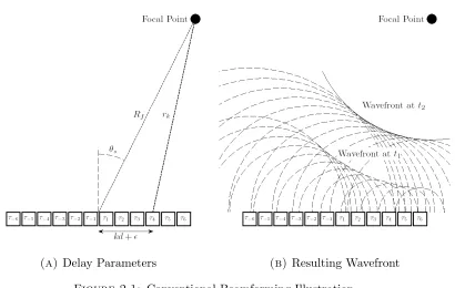
focal point. Figure 2.1 shows a one dimensional array that is focused at the focal

point shown. the elements are excited with a delay parameter according to the

(a) Delay Parameters (b) Resulting Wavefront

Figure 2.1: Conventional Beamforming Illustration

τk =

q

R2

f + (kd+)2−2Rfkdsin(θs))−Rf

c (2.1)

where τk is the time delay applied to the kth element, Rf is the distance between

the focal point and the center of the array as shown in Figure 2.1a, d is the pitch between the elements, θs is the angle between the normal to the array plane and

the focal point as shown in Figure 2.1a, and c is the speed of sound in the target

media.

Figure 2.1b shows the wavefront at times t1 and t2 after all elements have been

excited, where t1 < t2. It is clear that the waves from all elements will intersect at a later time at the focal point.

Such time delay scenario can be generalized to focus a 2-D array in a 3-D volume

Once the beam is focused onto a point in space, the energy of the constructively

interfered waves is high enough that a noticeable reflection can be observed if a

boundary is present. To image a volume, the ultrasonic array is focused at several

points in the target media, and the reflections are collected to compose a 2-D

image or a volume tomography.

In many cases this image needs further processing to clarify it in order for a

physician to make a diagnosis. This process is refereed to as post-processing and

has been tackled since the advent of ultrasonic imaging.

2.2

The convolution model

One of the major advancements in the field of post-processing in medical

ultra-sonography is the introduction of a convolution model from the standard wave

equation using the first-order Born approximation [30–36].

The convolution model states that the acquired B-Scan, which contains many

Radio-Frequency lines (RF-lines), y(n) can be displayed as:

y(n) =x(n)∗h(n) +η(n) (2.2)

wherex(n) is the Point Spread Function (PSF) that is produced by the transducer,

h(n) is the tissue response function representing the reflections at each boundary, andη(n) is any additive white noise present in the system. In many cases,η(n)≈0 and the noise in the system is convoluted noise present in h(n).

This model has been revolutionary in the field of ultrasonic digital signal

process-ing as solvprocess-ing for h(n) with the least amount of error results in a clear image of the target organ. It is important to note that the convolution model is a

The Point Spread function cannot be assumed to be the original transmitted

sig-nal. In ultrasonic imaging, the PSF exhibits a spatial dependency due to the

non-uniformity of focusing, diffraction effects, dispersive attenuation, and phase

aberrations [37–40]. Thus, the PSF has to be estimated in each B-scan in order

to acquire the tissue response function. In fact, in some cases PSF has to be

esti-mated in each section of the B-scan to accommodate for the spatial dependency

it exhibits.

The generalized convolution model also assumes a linear relation between the

acoustic field and the targeted biological tissue, which is not true as the linear

relation can only occur on conditions of weak scattering [41].

Even in the presence of the limitations to the Convolution Model mentioned above,

it can still provide a relatively accurate estimation. In order to solve for h(n), advanced digital signal processing techniques have to be applied instead of applying

conventional deconvolution.

Because of the nature of PSF in ultrasonography, the most effective way to

ex-tract the tissue response function in post-processing is through blind-deconvolution

[42]. Blind deconvolution can be achieved by either estimating the PSF first then

applying non-blind deconvolution[43], or by directly finding the tissue response

function.

In upcoming sections, the most commonly used post-processing techniques in

ul-trasonography are introduced. Section 2.2.1 and 2.2.2 follow the approach that

relies on finding an accurate estimation of the PSF, then applying non-blind

decon-volution. Section 2.2.3 explains the adaptive filtering tool, which many non-blind

and blind deconvolution methods use. Finally, Sections 2.2.4 and 2.2.5 show two

2.2.1

PSF estimation via statistical modeling: the ARMA

Process

The convolution model can be solved by means of system identification[44, 45].

More specifically, PSF can be estimated statistically through the autoregressive

moving average (ARMA) model[46, 47]. This approach considers the PSFx(n) to be the impulse response of a linear time-invariant system that is defined by the

generic difference equation as follows:

y(n) =

p

X

k=1

a(k)y(n−k) +

q

X

k=0

b(k)h(n−k) (2.3)

In the context of the theory of system identification, equation 2.3 is known as the

ARMA model. This method is a generalization of autoregressive (AR) and moving

average (MA) models. AR is obtained by setting q= 0, and MA by settingp= 0.

Using the ARMA model in ultrasonography means that the PSF can be

calcu-lated by estimating the ARMA parameters {a(k)}p_k=1 and {b(k)}q_k=1. After those parameters are estimated, the tissue response function can be found by means of

non-blind deconvolution.

Since the z-transform X(z)≡P∞

n=0x(n)z

−n _{of x(n) is given by:}

X(z) = B(z)

A(z) =

1 +Pq

k=0b(k)z −k

1 +Pp

k=0a(k)z−k

(2.4)

Estimating ARMA parameters can be done through maximum likelihood

estima-tion [45]. When the number of data points is relatively small, as is the case in

ultrasonography, this method proves inefficient. Other solutions that have been

proposed suggest minimizing the sum of squares of the one-step-forward prediction

error within the sampling range. The estimates are referred to as the Least square

It is important to note that although the ARMA process proves successful in many

cases in ultrasonic application, it assumes that the system is time-invariant. This

leads ARMA model to be susceptible to noise, and so it is important to either

filter the noise beforehand or restrict the use of the ARMA model to non-noisy

data.

2.2.2

Homomorphic estimation of PSF: the Cepstrum Model

The most common way to find PSF is using Homomorphic signal processing [49], or

more specifically, the cepstrum based methods for estimating PSF [35, 38, 46, 50–

52].

The method applies a Non-linear mapping to the cepstrum domain in which a

linear filter (referred to as a lifter) is applied and then a non-linear mapping is

applied to return the signal to the original domain.

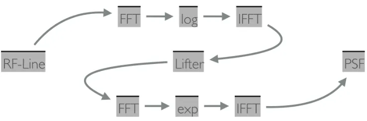
The cepstrum model, unlike the ARMA model, is a non-parametric model that is

used to extract PSF from RF-line or B-scan. The procedure is shown in Figure

2.2.

Consider the convolution model stated in equation 2.2 in the Fourier Domain:

Y(f) = X(f)·H(f) (2.5)

where upper case denotes their lower case counterparts after applying a Discrete

Fourier Transform[43]. In this case the pulse spectrum is convoluted with the

reflection spectrum. In order to separate the two, the logarithm is taken:

log(Y(f)) = log(X(f)·H(f))

=log(X(f)) +log(H(f))

=log|X(f)|+jarg(X(f)) +log|H(f)|+jarg(H(f))

In some simple cases, minimum phase can be assumed in X(f) and in H(f), and so, only the amplitude of those spectra are taken into consideration when

performing the following operations. This type of cepstrum analysis is referred to

as real cepstrum [50]. However, in ultrasonography, phase cannot be avoided due

to the non-negligible effects it has on the signal[35]; this is referred to as complex

cepstrum. To convert to the cepstrum domain, one must apply an inverse fourier

transform to the logarithm of the Fourier transform of the RF-line:

IF F T(log(Y(f))) = IF F T(log|X(f)|+jarg(X(f)) +log|H(f)|+jarg(H(f)))

= IF F T(log|X(f)|) +IF F T(jarg(X(f))) +IF F T(log|H(f)|

+IF F T(jarg(H(f)))

or

where the subscriptcrefers to the mapping of each of the variable in the spectrum domain to the cepstrum domain. Moreover, the subscript c, arg represents the phase contribution.

In the cepstrum domain, the PSF spectrum and the response function spectrum

are added instead of being convoluted. Thus, since the nature of the cepstrum

leaves the components of xc(n) at the lower portion of the cepstrum and the

components of hc(n) scattered across the sample, a simple low-pass lifter can be

applied to extract the signal xc(n) and its phase xc,arg(n).

Since a B-scan has multiple RF-lines, it is recommended to average all of the

results acquired after applying the lifter and before performing the mapping back

to the spectrum domain.

The conversion to the spectrum domain can be done by taking the Fourier

trans-form, applying the natural exponential, and taking the inverse Fourier transform.

Once PSF is acquired, deconvolution can be applied to reconstructh(n). At that point, the image is restored to a high quality. Deconvolution approaches that

can be used are ones acquired from a stable model, such as Lucy-Richardson

deconvolution and Weiner deconvolution.

2.2.3

Adaptive filtering tool and its application for

non-blind deconvolution

Adaptive filtering is a signal processing tool designed to converge on a solution for

an Unknown System given an input and the Desired Response as shown in Figure

2.3[3]. This tool relays on minimizing a cost function e(n), which is defined as the deference between the System Output and the “guessed” Network Response.

Figure 2.3: Basic Adaptive Filter for System Identification[3]

For example, in the case of non-blind deconvolution, xk can be considered the

estimation of the PSF, dk can be considered the RF-line y(n), and h(n) is the

unknown system.

To Identify the system, this process is taken:

1. xk is convoluted with some initial guess to produce the first Network

Re-sponse

2. The Error function is calculated by subtracting the Network Response from

the Desired Response and is inputted into the Adaptive Network

3. If the cost function has a large value, another guess is made. The new guess

is made using a learning algorithm that depends on both the value of the

cost function as well as other parameters

4. If the error function is small, then the Network Response is approximately

equal to the desired response, and so the guessed system is the unknown

There are many variables that can be changed to tailor the adaptive filter to one’s

needs. One of the main variables is the learning algorithm that is responsible of

changing the adaptive network in every iteration. The learning algorithm is most

commonly an intensive equation which takes into account the cost function, the

previous estimation of the network response, and many other variables. Chapter 3

shows that the learning algorithm is linear and the error function is not calculated

by simple arithmetic; rather, it is calculated after a mapping to a different domain

is done.

2.2.4

Blind-deconvolution via Single Input Multiple

Out-put Model (SIMO)

SIMO-based blind deconvolution is based on treating the echo response as a black

box whose input is the PSF and whose output is a collection of RF-lines[28]. In

this approach:

yk(n) =x(n)∗hk(n) (2.7)

Yk(f) =X(f)·Hk(f) (2.8)

X(f) = Yk(f)

Hi(f)

(2.9)

where the subscript k refers to the kth _{A-scan and the upper-case letters in 2.8}

refer to the DFT of their lower-case counterparts in 2.7. In this case, we do not

need information about X(n); we only need to solve for Hk(n). Thus, assuming

X(f) is a common variable for all A-scans:

Yi(f)

Hi(f)

= Yk(f)

Hk(f)

For N A-scans and N variables, this process produces N(N₂−1) equations. Since PSF may have spatial dependency, one can use only consecutive scans to estimate

the tissue response function.

2.2.5

Blind-deconvolution via Inverse Filtering

A popular Blind-deconvolution model is based on using the inverse filtering approach[53,

54]. Inverse filtering is based on restructuring the convolution model, then solving

for both the echo response and the inverse of PSF simultaneously. The convolution

model can be restructured as follows:

y(n) =x(n)∗h(n)

Y(f) =X(f)·H(f)

H(f) = 1

X(f) ·Y(f)

H(f) =S(f)·Y(f)

and so the restructured convolution model is:

h(n) = s(n)∗y(n) (2.10)

This restructured convolution model comes with two problems: the scale ambiguity

problem and phase ambiguity problem. The scale ambiguity arises from the fact

that the convolution model is

y(n) = 1

ax(n)∗ah(n) (2.11)

y(n) = x(n−no)∗h(n+n0) =x(n+n0)∗h(n−n0) (2.12)

wheren0 is an arbitrary constant. Those two problems can be solved by changing

the assumption of the restructured model to be

γh(n−n0)≈s(n)∗y(n) (2.13)

Estimating s(n) requires the assumption that h(n) is independent and identically distributed (i.i.d) and non-Gaussian random variable. This is essential as the

estimation method takes advantage of this assumption and builds on it.

Taking the central limit theorem into account, and because the PSF must be

Gaussian, the convolution between the Gaussian PSF and non-Gaussian h(n) is

always more Gaussian. The optimal inverse filter can then be determined using

this property to restore the non-Gaussianity of the data. To achieve this task, one

must minimize the entropy of the deconvolved result. This idea was first proposed

in [55] and implemented in [56].

In [55], maximizing the non-Gaussianity is done by the following:

sopt(n, m) = argmax s

P

n

P

m|(s(n, m)∗y(n, m))|

4

P

n

P

m|(s(n, m)∗y(n, m))|2

(2.14)

where m represents the mth _{RF-line and the corresponding tissue response}

func-tion. Although it has been proven to be an effective measure of non-Gaussianity,

using the forth moment in this manner may be problematic because of its inability

To improve the robustness of 2.14, [57] suggests generalizing the equation to find

an optimal filter using the following equation:

sopt(n, m) = argmax s

P

n

P

m|(s(n, m)∗y(n, m))|p

P

n

P

m|(s(n, m)∗y(n, m))|p/2

(2.15)

Another approach is the Claerbout’s measure and the resulting Claerbout’s

par-simonious deconvolution [58], which is based on inverse filtering with sopt defined

as:

sopt(n, m) = argmax s 1 N M X n X m

N M|(s(n, m)∗y(n, m)|2

P

n

P

m|(s(n, m)∗y(n, m)|2

×log

N M|(s(n, m)∗y(n, m)|2

P

n

P

m|(s(n, m)∗y(n, m)|2

(2.16)

Regardless which method is used from Equation 2.14, 2.15, or 2.16 the procedure

is always the same. An adaptive filter is used to carry out the calculation using

the steepest decent algorithm [59].

2.3

Conclusion: post-processing methods’

com-patibility for ultrasonic skull imaging

Methods mentioned in Section 2.2 are all outstanding approaches to the

convo-lution model in ultrasonography. However, in the case of skull imaging, these

methods encounter several difficulties. For example, the presence of the diploe

layer physically distorts the path of the beams. Thus, in the case of SIMO

(Sec-tions 2.2.4) and Inverse Filtering (Section 2.2.5), which relay on adjacent scans for

The most reliable approach for skull profile extraction is, therefore, to tackle each

RF-line separately, and filter out non-conclusive results. For this case, in order to

estimate h(n) as accurately as possible, a precise estimation of the PSF is criti-cal. Estimating the PSF can be done either through the ARMA Model (Section

2.2.1) or through homomorphic estimation using cepstrum (Section 2.2.2). After

estimating PSF it is necessary to perform deconvolution to acquire h(n). Adap-tive filtering shown in Section 2.2.3 is one of the most stable methods to perform

Non-blind deconvolution to acquire an accurate estimation of h(n). However, the deconvolution process proves more accurate for the cases where consecutive

reflec-tions are separated by a time delay larger than the pulse length. In skull imaging,

Adaptive filtering based deconvolution fails to locate the boundaries of the skull

since most of the reflections from the skull overlap.

In this study, a reliable and robust novel signal-processing technique, referred to as

the Selective Echo Extraction algorithm (SEE), is developed for the specific case of

ultrasonic skull imaging and accurate profile extraction. SEE does not relay on an

accurate pre-measurement of the PSF for clear results eliminating the effects of the

spatial dependence of PSF. In fact, only the acquisition system specifications and

a rough estimate of the skull’s acoustical properties are essential for the process.

The method is capable of disregarding the distortions caused by the diploe layer,

reviving reflections off of the skull-brain boundary, and accurately measuring the

skull’s inner boundary and its variable thickness across the examination area.

Additionally, a proposed method that utilizes SEE is shown to be able to measure

Theory and simulations

Acquiring skull profile from a distorted ultrasonic B-Scan proves quite difficult

using conventional signal processing techniques. This chapter introduces a novel

method for blind-deconvolution to acquire a clear image of the skull’s innermost

curvatures. The suggested Selective Echo Extraction Algorithm (SEE) can be used

to accurately detect both inner and outer curvatures of the skull. Furthermore,

SEE can be utilized to attain the average attenuation coefficient of the skull.

Chapter 3 is divided into four sections: Section 3.1 introduces the algorithm and

thoroughly discusses its details, Section 3.2 shows simulation results of B-Scans

processed through SEE and the custom-designed curve fitting method used to

acquire a correct curvature of the skull, Section 3.3 shows how SEE can be utilized

to determine the attenuation coefficient in the skull, and Section 3.4 discusses

the importance of SEE and the potential for its applications in ultrasonic

post-processing.

3.1

The Selective Echo Extraction algorithm

For the case of ultrasonic skull profile extraction, current conventional methods

for post-processing of RF data from the probed skull segment do not produce

accurate results as discussed in Chapter 2. For this reason, the Selective Echo

Extraction (SEE) algorithm has been developed and reported in this thesis. The

skull structure by nature, as discussed in Section 1.5, has three layers. The middle

layer which is referred to as “diploe” causes first and second strong reflections

that could be mistaken for the second boundary of the skull structure when using

conventional methods. SEE is a signal processing technique that is based on

extracting only useful information from a noisy ultrasound scan obtained from a

skull geometry.

The convolution model discussed in Chapter 2 states that:

y(n) = x(n)∗h(n) (3.1)

where y(n) is the collected A-Scan, x(n) is the point spread function, and h(n) is the tissue response function. The convolution model in the skull portion of the

A-Scan can be further expanded as follows.

y(n) = x(n)∗(hb(n) +hd(n) +hη(n)) (3.2)

where hb(n) represents the portion of the reflectivity function representing the

inner most and the outer most boundaries of the skull,hd(n) represents the

reflec-tions caused by diploe, and hη(n) represents the noise in the response function.

The goal of the SEE is to extract hb(n) and disregard all unnecessary information

included in the reflectivity function. In order to do so, SEE is created as per

the adaptive filter model and is tailored to the needs of the proposed convolution

in Algorithm 1 and each step in the Algorithm is thoroughly discussed to show

the physics and calculations performed to achieve the desired results.

Algorithm 1 The Selective Echo Extraction Algorithm

Input: y,Fc, BW, N,zf,d,W, cs, ρs,α,dmin, dmax

. y: Normalized RF-line in time domain.

. Fc,BW: The central frequency and bandwidth of the transducer [MHz]

. N,zf: The number of elements used to focus. and the focal distance [m]

. d,W: The pitch and element size of the transducer [m]

. cs,ρs, α: The speed of sound

_m

s

, density_mkg3

, and attenuation coefficient

N p mMHz

of the skull

. dmin, dmax: The minimum and maximum thicknesses of the skull.

Output: hb

. hb: The reflectivity function corresponding to outer boundaries of the skull

1: σω = _{2.67BW f}1 _c

2: xˆ=e−

t2

2σ_ω2

3: t1 = argmax(y) . the skull’s outermost boundary

4: fort=t1+ (dmin:dmax)/cskull do

5: reset ˆh

6: hˆ(t1) = 1

7: hˆ(t) = _N1 PN

n=1

sinc

W|N₂+1−n|dfc

tc2

s

e−2α

q

(|N+1 2 −n|d)

2

+(t−t1)2c2s

e−

t− q

(|N+1 2 −n|d)

2

−t2_c2

s−zf

/c

2

/(2σ2

ω)





2csρs

csρs+cwρw

2

csρs−ctρt

csρs+ctρt

8: yˆ= ˆx∗ˆh

9: cyyˆ=y ?yˆ

10: cyyˆ(n) =cyyˆ(n−argmax(cyyˆ))

11: e(t) =max|cyyˆ(t)−cyyˆ(−t)|

12: if e contains a global minimumthen

13: t2=t1 + argmin(e) . skull’s innermost boundary

14: reset ˆh

15: tˆ1= 1

16: ˆh(t2) = _N1 PNn=1

sinc

W|N+1₂ −n|dfc

t2c2s

e−2α

q

(|N+1 2 −n|d)

2

+(t2−t1)2c2s

e−

t2−

q

(|N+1 2 −n|d)

2

−t2 2c2s−zf

/c

2

/(2σ2

ω)





2csρs

csρs+cwρw

2

csρs−ctρt

csρs+ctρt

17: break

18: end if

In order for SEE to commence, only elementary information is needed along side

the A-Scan. Mainly, information related to experimental setup such as the

trans-ducer’s central frequency, bandwidth, pitch, element size, the number of elements

used for focusing, and the focal distance. Additionally, information is needed

about the target media, in this case the skull, such as the attenuation coefficient,

the speed of sound, and a rough estimation of the skull’s minimum and maximum

thicknesses. These properties, except the speed of sound, can be roughly estimated

and will not reduce the accuracy of the method. The speed of sound, however, is

a key property that is used to convert the samples from time based to distance

based via the basic formulad=ct, thus, must be provided with the least amount of error.

The behavior of the point spread function (PSF) is well known in ultrasound to be

a Gaussian modulated sinusoidal waveform [4]. The waveform of PSF is produced

by the vibration of a piezoelectric element as a response to an applied square

electric pulse.

In a blind deconvolution problem, as discussed in Chapter 2, it is essential to

estimate the PSF before applying deconvolution or to estimate the PSF

simulta-neously with the reflectivity function. However, Since SEE is a numeric method

rather than deterministic, it is unnecessary to estimate both aspects of the PSF:

Gaussian and sinusoidal. Therefore, additional processing can be avoided by only

estimating the portion of PSF with the dominant effect: the Gaussian portion.

The variance of the Gaussian portion of PSF can be calculated directly from the

frequency and bandwidth of the transducer as follows:

σω =

1 2.67BWfc

(3.3)

ˆ

x=e−

t2

2σω2 (3.4)

where σω is the pulse width of the excitation signal. It is important to note that

the estimated PSF is not claimed to fully represent the original PSF, rather is

used only for calculations inside the algorithm.

In an ideal experimental or clinical setup, reflections are expected to occur at the

following boundaries: the coupling medium and scalp boundary, the scalp and

skull boundary, the different layers of the skull, and the skull and brain boundary.

An estimation of the reflection at each boundary is described by the reflection

coefficient formula for normal incidence:

R = Z1 −Z2

Z1+Z2

(3.5)

whereZ1andZ2 represent the acoustic impedance of the first and second media at a specific boundary, respectively. The transmission coefficient, on the other hand,

is:

T = 2Z2

Z1+Z2

(3.6)

such that the R+T = 1. The acoustic impedance, Z, is defined as:

Z =ρc (3.7)

whereρ is the density in the medium, and cis the speed of sound in the medium.

In medical application, transducers are mostly designed to be water or tissue

cou-pled. Thus, at the coupling medium-scalp boundary, the impedance difference

most of the wave is transmitted. At the scalp-skull boundary, however, the

reflec-tion coefficient is rather high since the difference between the acoustic impedances

is high (Ztissue ≈ 1.6×106

kg m2_s

while Zbone ≈ 6.2×106

kg m2_s

)[65, 69]. Thus,

it is fair to state that the reflection with the highest amplitude in the A-Scan

occurs at the scalp-skull boundary. This fact is utilized in the algorithm at line 3,

where the first boundary of the skull is shown to be at the location of the highest

peak. Additionally, since the y is normalized, the amplitude of the first peak in the reflectivity function must be unity as shown in line 6.

To find the outermost boundary of the skull, the algorithm loops through various

proposed second boundary locations ranging from the minimum to the maximum

possible thickness provided. Thereafter, the algorithm performs calculations to

determine the most accurate estimation of the location of the second boundary.

The loop is performed in line 4 of Algorithm 1. Since in any given A-Scan the

acquired date is in units of time rather than distance, the loop is performed in the

time domain.

For each proposed location of the outermost boundary, the amplitude of the

re-flection must be calculated to properly perform comparison between the original

A-Scan and the proposed A-Scan. The amplitude of this reflection is dependent

on the distance from the first reflection, the nature of the skull, and the nature of

the wave. Each of these factors which contribute to the amplitude of the reflection

are discussed bellow.

Although the diploe layer of the skull is not considered to be a homogeneous

medium, the compact bone layers is composed from a dense homogeneous material

[2, 60]. Consider the propagation of a wave in a solid lossy medium [4, 61]. The

pressure,p, wave propagation in a homogeneous medium is expressed as follows:

∇2_p− 1 c2

∂2_p

Figure 3.1: Geometry defining the coordinate system for the Fraunhofer ap-proximation for a rectangular transducer.[4]

where cis the phase velocity at a reference frequency ofω, andL(t) is the convo-lutional loss operator that guarantees causality and which accounts for the effects

of dispersion and attenuation. The integral solution to this equation in the z

direction can be expressed as:

p(z :t) = 1 2π

Z ∞

−∞

p(0 : ω)e−i(ωc−iα(ω))zeiωtdω (3.9) wherepis the phasor pressure produced by the transducer andαis the attenuation coefficient as a function of angular frequency ω.

The phasor pressure can be calculated using the Fraunhofer Approximation [4].

For a rectangular transducer, The phasor pressure is given by:

p(x0, y0, z :w) = ωρ0c0

2πR e −ik

z+x

2 0+y20

2z

W Hsinc

W x0 λz

sinc

Hy0 λz

(3.10)

where W, H, R, x0,y0, and z are as shown in figure 3.1, and λ is the wavelength

Figure 3.2: One transducer element used to image a simple two media sample.

Thus the pressure produced by one rectangular element in a lossy medium with

attenuation coefficient α(ω) is:

p(x0, y0, z :t) = ωρ0c0 4π2_Re

−ik

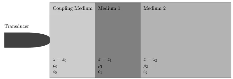
z+x

2 0+y20

2z

W Hsinc

W x0 λz

sinc

Hy0 λz

e−α(ω)z (3.11)

Equation 3.11 can be tailored to calculate the amplitude of peaks in A-Scans

undergoing certain conditions. For example, in a simple case shown in figure 3.2,

a transducer consisting of one rectangular element is used to acquire an A-Scan of

a system consisting of two media. In a normalized A-Scan, the amplitude of the

pressure at the first boundary is set to unity p(z1) = 1 such that the reflectivity

function at that location is 1: h(z1) = 1. Thus, to calculate the amplitude at the

boundary between Medium 1 and Medium 2 the following computations must be

incorporated: the pressure at z1, the pressure at z2, the transmission coefficient

at z1 and the reflection coefficient at z2. The observed second boundary location

corresponds to a reflection from normal incidence at x0 = 0 and y0 = 0. Since,

p(z) =e−α(ω)(z−z1) 2c1ρ1

c0ρ0+c1ρ1

(3.12)

The amplitude of the reflectivity function from a normalized A-Scan at z=z2 is:

h(z2) = e−2α(ω)(z2−z1)

2c1ρ1 c0ρ0+c1ρ1

2

c2ρ2−c1ρ1 c1ρ1+c2ρ2

(3.13)

The process discussed above can be extended to calculate the expected value of

the reflectivity function of more complex cases. In the case of an A-Scan acquired

from an N-element focused transducer, the pressure can be found by summing

over the pressure produced by each element. Note that if N is even, thexposition of the focal point at which the reflection is observed is between the central two

element, alternatively, if N is odd, thex position of the focal point is at the center of the central element. Thus, the x0 displacement between each element and the

observed point is:

xn=

N+ 1 2 −n

d (3.14)

where d is the pitch of the transducer. xn is substituted in equation 3.11 asx0 for

each transducer element. Additionally, it’s worth mentioning, that each element is

excited at different excitation time to produce a focal point as discussed in Section

2.1. The pressure of each element is also dependent on time of arrival and the pulse

width. Thus the pressure produced from N elements at a distance z1 < z < z2

and time t is given by:

p(z :t) = 1

N N X n=1 sinc

W xn

λz

e−2α(ω)

√

x2

n+(z−z1)2_e− (t−tn)2

2σ2_ω

2c1ρ1 c0ρ0+c1ρ1

where the time delay is given by:

tn =

p

x2

n+z2−zf

c (3.16)

where zf is the distance at which the transducer is focused. If z = z2 then the

reflection coefficient has to be considered as well a second transmission coefficient.

Thus, the amplitude of the reflectivity function from a normalized A-Scan atz =z2

is:

h(z2) =

1 N N X n=1  sinc

W xn

λz

e−2α

√

x2

n+(z−z1)2_e−

(z₂ c₁−tn)

2

2σ2ω





2c1ρ1 c0ρ0+c1ρ1

2

c2ρ2−c1ρ1 c1ρ1+c2ρ2

(3.17)

Line 7 of Algorithm 1, corresponds to an expanded form of equation 3.17 in terms

of the variables available in the algorithm. Line 7 states:

ˆ

h(t) = 1

N N X n=1 " sinc W

N₂+1 −n df_c

tc2

s

!

e−2α q

(|N+1 2 −n|d)

2

+(t−t1)2c2s

e−

t− q

(|N+1 2 −n|d)

2

−t2_c2

s−zf

/c

2

/(2σ2

ω)

#

2csρs

csρs+cwρw

2

csρs−ctρt

csρs+ctρt

(3.18)

This completes the estimation ofhb which is referred to as ˆhin the algorithm. The

estimate of the A-Scan corresponding to the two skull boundaries, ˆy, is calculated in line 8 as the convolution of ˆx and ˆh. In line 9, the cross correlation between the original and the proposed signals is calculated and in line 10 the cross correlation

function is centered about its maximum point. The centering is important to

ensure that the first reflections in the original and proposed A-Scans are perfectly

aligned.

g(t) at another time. Therefore, Cross-Correlation in line 9 provide a description of the similarity between the estimated signal and the original. Cross-correlation

is calculated as follows[3]:

rf g(τ) = lim T→∞

1

T

Z T

0

f(t)g(t+τ)dt (3.19)

whererf g(τ) is the cross correlation between the functions f and g at time τ, and

T is the total observation time. To show the necessity of using cross correlation to compare the original A-Scan and the proposed A-Scan two cases are shown bellow.

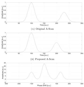
Consider a hypothetical A-Scans with a PSF of Gaussian nature and two distinct

reflections as shown in figure 3.3a. Assume the proposed estimation of the

A-Scan is as shown in figure 3.3b. Then the Cross-Correlation between the original

and the proposed A-Scan is given in figure 3.3c. The high peak in the center of

the cross-correlation is a product of the first reflection from each A-Scans added

to the product of the second reflections from each A-Scans. This is because the

highest correlation between the two A-Scans happens at zero shift. The peak on

the right side in the correlation, however, represents the product between the first

reflection of the proposed A-Scan and the second reflection of the original A-Scan

thus representing the behavior of the original A-Scan post the first peak. Similarly,

the peak on the left side represents the correlation between the first reflection of

the original with the second reflection of the proposed A-Scan.

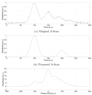
This convention is also shown in figure 3.4, where figure 3.4a contains the

origi-nal A-Scan including many reflections and uniformly distributed error, and figure

3.4b contains the proposed A-Scan including only two reflections. It is safe to

assume from these two cases that the right hand side of the correlation represents

the original A-Scan behavior post first peak while the left hand side represents

the proposed’s A-Scan’s behavior post first peak. Moreover, the cross-correlation

produces results with no error which is essential in scans with low signal to noise

(a) Original A-Scan

(b) Proposed A-Scan

(c) Cross-Corrolation between the original A-Scan and the proposed A-Scan

Figure 3.3: Cross-Correlation example for a hypothetical simple case of A-Scans with a Gaussian PSF

It is important to note that the similarity between the two sides of the correlation

is maximum when ˆy best describes the hb portion of the A-Scan. Therefore, the

two sides of the correlation can be effectively used to produce an error factor

between the proposed A-Scan and the Original. The error factor e(τ) is defined in line 11 as:

e(τ) = max|cyyˆ(t)−cyyˆ(−t)| (3.20)

(a) Original A-Scan

(b) Proposed A-Scan

(c) Cross-Corrolation between the original A-Scan and the proposed A-Scan

Figure 3.4: Cross-Correlation example for a hypothetical complex case of A-Scans constructed with a Gaussian PSF and added uniformly distributed

random error

A-Scan ˆy. e(τ) provides an illustration of the difference between the the original A-Scan and a proposed A-Scan where the proposed A-Scan contains only two

peaks separated by time shift τ.

In every iteration shown in line 4 of the algorithm, a new A-Scan is proposed and

the error for the time shift is calculated. After a few alterations, the process of

detecting the highest similarity (lowest error) starts.