Arithmetic Using Word-wise Homomorphic Encryption
Gizem S. C¸ etin1, Yarkın Dor¨oz1, Berk Sunar1, and William J. Martin1
Worcester Polytechnic Institute {gscetin,ydoroz,sunar,martin}@wpi.edu
Abstract. Homomorphic encryption has progressed rapidly in both efficiency and versatility since its emergence in 2009. Meanwhile, a multitude of pressing privacy needs — ranging from cloud computing to healthcare management to the handling of shared databases such as those containing genomics data — call for immediate solutions that apply fully homomorpic encryption (FHE) and somewhat homo-morphic encryption (SHE) technologies. Further progress towards these ends requires new ideas for the efficient implementation of algebraic operations on word-based (as opposed to bit-wise) encrypted data. Whereas handling data encrypted at the bit level leads to prohibitively slow algorithms for the arith-metic operations that are essential for cloud computing, the word-based approach hits its bottleneck when operations such as integer comparison are needed. In this work, we tackle this challenging prob-lem, proposing solutions to problems — including comparison and division — in word-based encryption via a leveled FHE scheme. We present concrete performance figures for all proposed primitives.
Keywords:Homomorphic encryption, word-size comparison, homomorphic division.
1 Introduction
Afully homomorphic encryption scheme (FHE scheme) is one which permits the efficient evaluation of any boolean circuit or arithmetic function on ciphertexts [21]. One easily checks that we can model a universal set of gates using addition and multiplication over any non-trivial ring convenient to us. Gentry introduced the first FHE scheme [9, 10] in 2009; this lattice-based scheme was the first to support the efficient evaluation of arbitrary-depth boolean circuits. This was followed by a rapid progression of new FHE schemes (e.g., [25, 4, 24]). In 2010, Gentry and Halevi [11] presented the first actual FHE implementation along with a wide array of optimizations to tackle the infamous efficiency bottleneck of FHE schemes. Further optimizations for FHE which also apply to somewhat homomorphic encryption (SHE) schemes followed including batching and SIMD optimizations; see, e.g., [12, 23, 13]. Nevertheless, bootstrapping [10], relinearization [5], and modulus reduction [5, 4] remain as indispensable tools for most HE schemes.
Most relevant to the present work, L´opez-Alt, Tromer and Vaikuntanathan proposed SHE and FHE schemes (which we denoteLTV) based on the Stehl´e and Steinfeld variant of the NTRU scheme [24]; LTVsupports inputs from multiple public keys [19]. Bos et al. [1] introduced a variant of the
LTV FHE scheme along with an implementation. The authors of [1] modify the LTV scheme by adopting a tensor product technique introduced earlier by Brakerski [3] thereby providing a security reduction to that of standard lattice-based problems. Their scheme affords enhanced flexibility by use of the Chinese Remainder Theorem on the message space and obviates the need for modulus switching. Dor¨oz, Hu and Sunar propose another variant of theLTVscheme in [8], putting forward a batched, bit-sliced implementation that features modulus switching techniques.
reduction, and thresholding. Meanwhile SHE tools, developed mainly to achieve FHE, have not been sufficiently explored for use in applications in their own right. In [20] for instance, Lauter et al. consider the problems of evaluating averages, standard deviations, and logistic regression which provide basic tools for a number of real-world applications in the medical, financial, and advertising domains. The same work also presents a proof-of-concept Magma implementation of an SHE scheme, offering basic arithmetic functionality, based on the ring learning with errors (RLWE) problem proposed earlier by Brakerski and Vaikuntanathan. Later, Lauter et al. show in [16] that it is possible to implement genomic data computation algorithms where the patients’ data are encrypted to preserve patient privacy. The authors used a leveled SHE scheme which is a modified version of [18] where they omit the costly relinearization operation. In [2] Bos et al. show how to privately perform predictive analysis tasks on encrypted medical data. These authors use the SHE implementation of [1] to provide timing results. Around the same time, Graepel et al. demonstrate in [14] that it is possible to homomorphically execute machine learning algorithms in a service while protecting the confidentiality of the training and test data. They, too, provide benchmarks for a small scale data set to show that their scheme is practical. Cheon et al. [7] present a method along with implementation results to compute encrypted dynamic programming algorithms such as Hamming distance, edit distance, and the Smith-Waterman algorithm on genomic data encrypted using a somewhat homomorphic encryption algorithm.
2 Motivation
With word size message domains we gain the ability to homomorphically multiply and add integers via simple ciphertext multiplications and additions, respectively. This significant gain comes at a severe price. We can no longer homomorphically compute a zero test via direct evaluation of a standard boolean comparator circuit, since the input bits are no longer accessible via our homo-morphic evaluation operations. The same applies to more complex operations such as comparison evaluations, thresholding and division. Division, in particular, requires heavy computations and is challenging to evaluate in either bit or higher characteristic encryption. Therefore, it is commonly avoided by selecting division free algorithms or by postponing the computation to the client side after decryption whenever possible.
Our Contribution. In this work we present an array of solutions to improve the versatility of higher characteristic SHE/FHE schemes along with new abilities, specifically:
– We compare three approaches to field inversion, each with its advantages; these naturally lead to algorithms for division, zero test and equality checking. The first method is exact but slower; the others produce rational approximations, which we scale to integers. Our approach based on Newton-Raphson iterations also gives us an algorithm for square roots. Our convergence-based approach performs better when the characteristic is large due to their amenability to residue number system-based optimizations. Particularly valuable by-products include comparison cir-cuits and threshold functions.
– We discuss the usage of residue number system (RNS) representation for proposed arithmetic operations to achieve a large message space. The operations that output encodings of rational approximations are not compatible with such economies: slight differences in such pre-rounded values can produce vastly different images under the CRT.
– We summarize with an overall comparison of word-wise homomorphic algebraic operations vis a vis their bit-wise counterparts for 32-bit integer domain.
– We implement the proposed methods using an LTV-based homomorphic encryption library and provide the execution times.
3 FHE Background
An FHE scheme is an encryption method where one is capable of performing these two primitive operations: Decrypt(c1+c2) = b1+b2 and Decrypt(c1·c2) =b1·b2 (where ci is the corresponding encryption ofbi). In general, all operations are performed over a ring of the formR=Zq[x]/hF(x)i with a prime modulus q and an irreducible polynomial F(x) with small coefficients. The schemes also specify an error distribution χ over R, typically a truncated discrete Gaussian distribution, for sampling random polynomials that are B-bounded whereB q. The term B-bounded means that the coefficients of the polynomial are selected in the range [−B, B] according to distribution χ: for g ← χ, we have kgk∞ ≤ B. There are usually four primitive functions, namely Keygen,
Encrypt,Decrypt andEval. Among these,Eval involves homomorphic multiplication, which creates significant noise growth in ciphertexts and in order to cope with this, there are also several noise cutting operations.
For advanced algebraic operations, we will build homomorphic circuits involving only additions and multiplications, hence our proposed algorithms are not designed for a particular FHE scheme. However, there are some optimization techniques that are specific to theLTV-variant DHS scheme that we used in our experiments.
3.1 DHS Variant of LTV Scheme and FLaSH Library
In 2012 L´opez-Alt, Tromer and Vaikuntanathan proposed a leveled multi-key FHE scheme (LTV) [19]. The scheme is based on a variant of the NTRU encryption scheme proposed by Stehl´e and Steinfeld [24]. The LTV scheme uses a new operation calledrelinearizationand existing techniques such as modulus switching for noise control. In this work, we use a customized single-key version of LTVproposed by Dor¨oz, Hu, and Sunar [8] along with key size reduction techniques. In this section, we describe an instance Lof FLaSH, the software library of the DHS scheme.
– L.Keygen first samples polynomials from B-bounded error distributionχ:f0 ← χ and g ← χ. Then it sets the secret key f = pf0 + 1, computes the public key h = pgf−1 and finally the
evaluation keysζτ =hsτ+peτ+wτf2 wheresτ, eτ ←χ,wis the relinearization block size and τ ∈[0,dlogq0/logwe −1]. All operations in this step are performed in ringR0.1
– L.Encrypt(m) =hs+pe+mwhere s←χ ande←χinR0.
– L.Decrypt(c(i)) = df c(i)cqi
p where c
(i) is the ith level ciphertext and the balancing operation
d·cqi reduces coefficients moduloq to lie between −q/2 andq/2. The last operation [·]p reduces the result modulo p to find the encrypted message. The operations are performed inRi. – L.Add(c(1i), c(2i)) =c(1i)+c(2i) inRi.
– L.Mult(c(1i), c(2i)) =c(1i)·c(2i) inRi. – L.Relin(c(i)) = P
τζτc
(i)
τ in Ri where c(i)(x) = Pτwτc(τi)(x) expands ciphertext c as a com-bination of polynomials with all coefficients in [0, w−1] for τ ∈ [0,dlogqi/logwe −1]. This operation simulates the homomorphic multiplication with the secret key, hence corrects the encryption mask hs after each multiplication, in addition to reducing the noise.
– L.ModSwitch(c(i)) = b˜c(i)/qep decreases the noise by logq bits by dividing the ciphertext coef-ficients by q. The operation b·ep refers to rounding so as to match all parities with respect to message domainp.
– L.Batch(m1, m2, . . . , mr) =
h Pr
i=1miFi
Fi−1
fi i
F packs multiple messages into a single plain-text polynomial for parallel evaluations as proposed by Smart and Vercauteren [23, 12]. For this purpose, we select a polynomial F(x) that factors over Fp into r irreducible polynomials fi(x) each of degree exactlyt. Then messages are embedded using the Chinese Remainder The-orem whereFi= fFi((xx)). When plaintext space p < n, we use F(x) =Ψm(x), hence we can batch r =n/tmessages into one polynomial, wheretis the smallest integer that satisfiespt−1m = 0 where m is the cyclotomic degree and ϕ(m) = n. When p > n, we use F(x) = xn+ 1 where [p−1]2n= 0.
For further details of the scheme, noise growth and security analysis, we refer readers to [8].
4 Beyond Additions and Multiplications
Most homomorphic encryption schemes provide, as basic functionality, addition and multiplication of ciphertexts which encrypt elements in some ring, with the caveat that multiplication gates are considerably “more expensive” than addition gates. At face value, this equips us with the ability to evaluate multivariate polynomials on inputs with a strong preference for low degree polynomials.
In applications such as machine learning, other fundamental operations become essential: di-vision,zero test,thresholding and comparison. Bit-level encryption excels at functions with Boolean output but incurs prohibitive cost when required to perform arithmetic even in moderate-sized message domains. Approaching this from the other end, we seek out algebraically efficient algorithms for the operations in the above list. Our solutions fall generally into three categories:
– algebraic and exact algorithms;
– approximation-based algorithms with variable precision outputs;
1
Note that due to the choice of moduliqi, all keys can be promoted to the next levels using modular reduction, i.e. h(i)= [h]
qi,f (i)= [f]
qi andζ (i) τ = [ζτ]q
– an ad hoc technique for efficient division of polynomial coeffcients by a prescribed constant.
We begin with three approaches to inversion, which become the basis for more advanced operations later in the section. Section 5 concludes with a summary of how and when RNS-based techniques can be employed to parallelize and/or speed up the execution of these tools as well as expand the message space to avoid overflow.
4.1 Multiplicative Inverse and Division
One of the most difficult, and currently open, questions is how to implement homomorphic division efficiently. With bit-level encryption, one could implement a parallel division circuit by unrolling the shift and subtract operations. However the depth of this division circuit would be very high; the best we can do is to use a costly carry-lookahead subtraction circuit and emulate a serial shift division algorithm with depth complexity O(nlog(n)). In the case of higher characteristic, we run into the aforementioned comparison and sign-detection problems.
The problem is as follows: Given two inputs a and b which are both defined in Zp, can we
find a polynomial function, P(x, y) say, such that P(a, b) = a/b? This question can be reduced to this: Can we find a polynomial P(x) such that P(b) = 1/b? Because if there exists such P(x), then in order to find a/b, we can computeaP(b) =a/b. Furthermore the same polynomial can be used to execute a simple zero test which we will describe later. In this section we will construct such a polynomial using three different methods. The first one gives an exact algebraic solution, but works as a modular operation, whereas the next two use approximation algorithms and they output real-valued results with respect to a preinitialized precision.
Fermat’s Little Theorem We can obtain a polynomial function via Fermat’s Little Theorem that permits homomorphic evaluation of the multiplicative inverse b−1 of a number b, modulo p. Note that a generalization of Fermat’s Little Theorem states thatbα≡bβ mod pas long as α≡β mod ϕ(p), whereb andp are coprime. If we pickpa prime, bcan be any number fromZp and it is known that ϕ(p) =p−1. It follows thatb−1 modϕ(p)=bp−2 mod p. Hence we define P(x) =xp−2
and P(x) is defined over Zp.2
Lemma 1 (Modular Inverse and Modular Division). Let L=LTV(p, q) where p ∈ Z is prime. For c = L.Encrypt(b), we compute c˜= cp−2. Then L.Decrypt(˜c) = b−1 mod p. For c1 = L.Encrypt(a), c2=L.Encrypt(b), if we computec˜=c1cp2−2, then L.Decrypt(˜c) =ab−1 mod p.
As we have a polynomial of degree p −2, this method is not very efficient due to the fact that we have to compute a homomorphic exponentiation of multiplicative depth O(log(p)). Unless p is small without further customization this approach will not be very practical. Additionally note that this method does not provide a multiplicative inverse over real numbers since this is a modular operation. On the bright side, the output is an exact arithmetic solution, i.e., there is no approximation, no fractions or precisions to handle. In the next approach we will find the reciprocal, not simply modulop, but as a real number using a root finding algorithm.
2
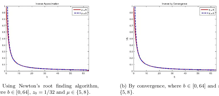
Newton’s Root Finding Algorithm We can find the multiplicative inverse of any arbitrary numberbusing Newton’s root finding algorithm. The functionf(z) = 1/z−bhas a root atz= 1/b, hence if we can find the root of f(z), we obtain the reciprocal for b. Iterations start with an initial guess z0 and follow by finding zi+1 = zi− ff0((zzi)i) = zi(2−bzi). Assuming b lies within the range [0,2k], we set the initial valuez0 to 21−k and fix the number of iterations toµ; the approximation
can be seen in Figure 1a.
For this and upcoming algorithms, we employvariable precisionrepresentations. More precisely, our ciphertexts will encrypt integers which give correct results only when scaled down and rounded to the nearest integer. We therefore implicitly have a new data type for homomorphic computation. An ordered pair (c, u), where c = Encrypt(m) and u is a non-negative integer, is viewed as an encryption of the integer dm/2uc obtained by rounding Decrypt(c)/2u. The integer u specifies the location of the (binary) precision point; bits to the right of this point are viewed as a sort of noise. Adding or subtracting two such ciphertexts requires us to align their precision points: for (c, u) and (c0, u0) with u0 > u, the sum is represented by (c2u0−u +c0, u0). Likewise, multiplication of ciphertexts (c, u) and (c0, u0) yields (cc0, u+u0). In what follows, the u+u0 fractional bits of the corresponding plaintext will be rounded to the nearest integer. Note that, with Zp as our message domain, we have u≤logp.
Applying this framework to our Newton iterates, we encode/represent z0 = 21−k as (1, k) and
set ¯z0 = 1. With ρ = 2k−1, we then represent the rational number z1 = z0(2−bz0) as (¯z1,2k)
where ¯z1= ¯z0(2ρ−bz¯0) so decryption gives the rounded valuedDecrypt(¯z1)/22kcuz1 after the 2k
fractional bits are removed. Continuing in this manner, we represent z2 =z1(2−bz1) as (¯z2,4k)
where ¯z2 = ¯z1 2ρ2−bz¯1
again doubling the number of fractional bits. The general form is then to represent zi+1 as (¯zi+1,2i+1k) where ¯zi+1 = ¯zi
2ρ2i−bz¯i
.
Lemma 2 (Approximate Inverse). Let L=LTV(p, q) and c = L.Encrypt(b) with 0 < b < 2k.
We set ¯c0= 1 and iteratively computec¯i+1= ¯ci
2ρ2i−c¯ci
, whereρ= 2k−1. Then for sufficiently large µ, L.Decrypt(¯cµ) u (1/b)ρ2
µ−1
mod p. Let d = L.Encrypt(a), we compute d¯= d¯cµ. Then
L.Decrypt( ¯d)u(a/b)ρ2
µ−1
mod p.
The depth of this approximation depends on the number of iterations µ, i.e., it is independent of p. Consider the equation ¯ci+1 = ¯ci2ρ2
i
−¯c2ic, the depth of the function comes from the product ¯
c2ic. Initially ¯c0 is a constant, hence the exponent ofc in ¯c1 becomes 1. In the next iterations, the
(a) Using Newton’s root finding algorithm, whereb∈[0,64],z0= 1/32 andµ∈ {5,8}.
(b) By convergence, whereb∈[0,64] andη∈ {5,8}.
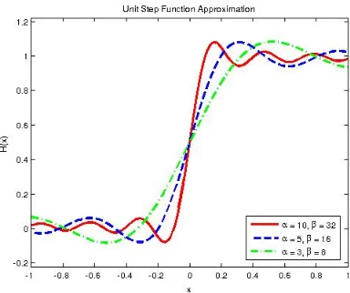
Fig. 1: Multiplicative inverse approximation functionP(x) = 1/x
Goldschmidt’s Convergence Method We briefly and informally describe how to find the inverse by convergence as follows: Assume we want to compute the reciprocal 1/b. The algorithm works by multiplying both the numerator and denominator by a series of valuesr0, r1, . . .so as to make the
denominator converge to 1. Thus, at the end of the computation the numerator yields the desired division result:
1 b =
1 b ·
r0
r0
·r1 r1
· · ·rη rη
, b·r0r1· · ·rη →1 .
The standard approach starts by normalizing 1 and b to become fractions in the unit interval, in particular b ∈ [12,1). Then we can write z = 1−b where z ∈
0,12. Then setting r0 = 1 +z,
r1 = 1 +z2, . . . , ri = 1 +z2
i
will yield the desired result. We can show that b·r0 ∈ [1−2−2,1],
b·r0r1∈[1−2−4,1], b·r0r1r2∈[1−2−8,1], etc., with productsb·r0· · ·rη converging to one. The approximated inverse values for differentη can be seen in Figure 1b.
Given ` and c = Encrypt(b) and setting σ = 2`, we can mimic the inversion by convergence algorithm to effect a homomorphic division operation. Our variable precision encoding associates the ordered pair (c, `) to b0 = b/σ. Next z = 1−b/σ is represented by (¯z, `) where ¯z = σ −c. Likewise, our representation for ri = 1 +zi is (¯ri,2i`) where decryption of ¯ri is close toσ2
i
ri. Putting this all together, we find that 1/bur0·r1· · ·rη/σis well approximated by P(b)/σ2
η+1
whereP(x) =Qη
i=0
σ2i+ (σ−x)2i
. So our variable precision approach represents our encryption of 1/bas (P(c),2η+1`) where the fractional part ofP(c) consists of the last 2η+1` bits.
For the most significant ` bits to stabilize, we need log(`) + log log(`) = O(log(`)) iterations which also represents the depth of the computation. Now if we cannot estimate the magnitude of b, due to repeated squaring the power ofz will double in precision in every iteration moving bit by bit closer to the end of the precision window3. Therefore, we will need another O(`) iterations for the denominator to reach 2i`−1 ≤br0r1. . . ri<2i`. In practice the number of iterations required by the division by convergence algorithm will depend on the distribution of the data. For uniformly distributed data of precision `, the expected value of the deviation in the magnitude will be in
the order of 2O(log(`)). Therefore, the average case and worst case complexities of the division by convergence algorithm are in the order ofO(log(`)) andO(`), respectively.
Lemma 3 (Approximate Inverse). Let L=LTV(p, q) and c =L.Encrypt(b). We compute ˜c =
Qη
i=0
σ2i+ (σ−c)2i
, for a chosen number of iterations η, which depends on the predetermined
precision factor`, with inputsb∈[0,2`]andσ = 2`. We haveL.Decrypt(˜c)u(1/b)σ2
η+1−1
mod p. Let d=L.Encrypt(a), we compute d˜=d˜c. ThenL.Decrypt( ˜d)u(a/b)σ2
η+1−1
mod p.
The polynomialP(x) has degreePη
i=02i = 2η+1−1 requiring a circuit of depth log 2η+1−1
= η+ 1. As in the previous approximation method, this is also independent of the message space size p. But both algorithms suffer from the growth in the fractions, i.e. p should be large enough to cover the magnitude of the end result in order to avoid overflows. Even with small precision, after a few iteration steps we end up with a large fraction. This is a generic problem in any approximation-based algorithm where we have to use real numbers. Thus, later in Section 5.2, we propose a method to make these schemes that require large p more practical using RNS. We also propose another solution, where we describe a homomorphic constant division method, so that we can adjust the precision before decryption. This method decreases the magnitude of p on the fly, hence there are advantages and disadvantages that will be discussed later. (See Section 5.1.)
4.2 Zero Test and Equality Check
We can obtain a polynomial function that permits homomorphic evaluation of a zero test. The test returns a zero or one depending on whether or not the ciphertext is (or rounds to) an encryption of zero. Let this polynomial beZ(x). Then we want to have Z(a) = 0 if ais equal to zero, Z(a) = 1 otherwise. We can retrieve this functionality using Fermat’s Little Theorem by computing xp−1 mod p. This can be interpreted as multiplying the input x with its inverse modulo p, which is xp−2 modp. Inspired by the same idea, we can create a zero test polynomial by using any inverse polynomial as follows: Z(x) = xP(x). Then the output will give us a 0 or ω depending on the chosen inverse finding method.
The zero test may be used trivially to homomorphically perform an equality check on two messagesa,b by computing Z(a−b). Note that this is a much simpler operation than magnitude comparison which we will address later in Section 4.3.
Lemma 4 (Zero Test and Equality Check). Let L=LTV(p, q) and c = L.Encrypt(b). We compute ˜c=cP(c). Then L.Decrypt(˜c) = 0 if b= 0 mod p and L.Decrypt(˜c)uω if b6= 0 mod p.
Let c1 =L.Encrypt(a) and c2=L.Encrypt(b), then if we computec=c1−c2 and ˜c=cP(c), we will retrieveL.Decrypt(˜c) = 0 if a=b modp andL.Decrypt(˜c)uω if a6=b mod p.
The degree of Z(x) is always one more than the degree of P(x). Thus, the complexity of a zero test depends on the underlying inverse polynomial. Due to the same reason, the zero test also suffers from the same problems of the chosen inverse method.
4.3 Thresholding and Comparison
a polynomial to represent this operation. Let it be T(x, t), then we want T(a, t) = 0 when a < t whereas T(a, t) = 1 otherwise. We can devise this algorithm by testing the equality over the range of integersi= 0, . . . , t−1 and aggregate the result as4 T(x, t) =P
i∈[t](ω−Z(x−i)) where Z(x)
is a zero test polynomial that is described in the previous section. Clearly, we can instead compute the complement if tis closer top than to 0.
If we compute it using Fermat’s Little Theorem, although it is not efficient, this presents a viable and exact technique for evaluating thresholds. A significant positive aspect of the formulation is that the multiplicative depth of the threshold computation is independent of the threshold constant tand is the same as the depth of an equality check: O(log(p)). On the other hand, the summation becomes computationally expensive — with complexityO(tlog(p)) — aspand the range oftgrow. Lookup tables and selection of special moduli can be used to increase the efficiency.
Unlesspis small without further customization this approach will not be very practical. To gain some economy over the primep case, we may chosep to be highly composite p=Q
i∈[k]pi in such a way that the zero test simply becomescϕ(p) =cQϕ(pi). Then the multiplicative depth complexity of a zero test (or comparison) becomesP
i∈[k]log(pi−1).
Approximation Methods In order to retrieve a threshold polynomialT(x), we will make use of the Unit Step Function, i.e H(x) = 0 when x < 0 and H(x) = 1 when x > 0, then we can just computeT(x) =H(x−t) wheretis a fixed cleartext threshold. Furthermore, the same polynomial can be used to compare two encrypted valuesa,bby computingH(a−b). We propose two different methods to create a step function.
For the first approach we will make use of logistic function and the equation is given as follows, H(x) = lim
k7→∞
1
1+e−2kx u (ex) 2k
1 + (ex)2k
−1
. By limiting k to a small constant, we can get a smooth approximation and we can use Taylor Series approximation to compute the exponential function ex
u P∞i=1 x i
i!, and we can also use one of the inverse functions that we found in
Sec-tion 4.1. Thus H(x) becomes: H(x) u
P∞
i=1 x i
i! 2κ
P
1 +P∞
i=1x i
i! 2κ
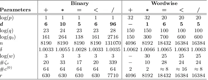
. Even though we can get a threshold polynomial using this approach, it is computationally expensive considering the in-put to the inverse function has already a large exponent. Therefore, we use another approach which is constructing a square wave using sine waves. Square wave functionS(x) can be approximated as, S(x)uP∞i=1
sin((2i−1)x)
(2i−1) For sinus values we can use the approximation, sin(x)u P∞
j=1
(−1)j−1x2j−1 (2j−1)! .
Embedding this in the previous equation we will have,S(x)uPj∞=1P∞i=1 (−1)
j−1(2i−1)2j−2 (2j−1)! x
2j−1
The output of the square wave function is in the range of [−0.8,0.8] in a period, thus we compute H(x) as: S(x1)+0.6 .8. The degree of H(x) depends on the upper limit for j. If we define i∈[1, α] and j∈[1, β], then the largest exponent of inputx, i.e., the degree ofH, becomes 2β−1. Consequently, the depth of the approximation algorithm becomesdlog (2β−1)e=dlogβe+ 1. For different values of α andβ the unit step approximation can be seen in Figure 2.
To make use of this approximation algorithm, we also need to associate message space elements to discrete samples of the input range [−1,1] of H(x). Assume we handle elements of precision ` bits and we want to findH(b−t), where b, t∈[0,2`). Then we have an inputx=b−t∈ −2`,2`
and we have to normalize it withω = 2`, so that the normalized value lies in the input range, i.e.
Fig. 2: Unit step functionH(x) for various approximation degrees.
x/ω ∈ (−1,1). As in the previous approximation methods, we need to represent` fractional bits with a binary point placed right after leaving a single bit for the integer part. During evaluation we need to keep track of the precision point which moves to the left, with each multiplication byx. Once the evaluation is completed the approximation result resides in the most significant precision bit(s) ready to be used for subsequent evaluation and the maximum number of fraction bits can be found in the term with the highest exponent,ω2β−1.
4.4 Square Root
We can find an approximation to the square root of a number by using a root finding algorithm. As before, we seek a polynomial, R(x) say, such that R(b) = √b. The function f(y) = y2 −b
has a root at y = √b, hence if we can find the root of f(y), we obtain the square root of b. If we use Newton’s Root Finding method as in Section 4.1, we can iterate through the values yi+1 = yi − ff0((yyi)i) = 12
yi+ybi
with an initial guess of y0. For the inverse computation ybi, we
can use the inverse approximation polynomial that we retrieved before, yi+1 = 12(yi+bP(yi)). In order to handle fractions, again we need to consider an imaginary precision point. The depth of the algorithm depends on the number of iterations, κ say; then total depth will be κ times the depth of the inverse computation P(x). Thus this is a much more costly operation relative to inversion.
5 Making Word Arithmetic More Practical
As mentioned before, most of the proposed methods require a largep. By increasing the size of p, we incur a high noise growth in the ciphertexts. As a consequence, this leads to the use of larger coefficient size for the ciphertexts, i.e., the ring R = Zq[x]/hF(x)i with a larger q. Increasing q
5.1 Constant Division - Adjusting the Precision
Here we introduce a technique that may be used to remove excess bits (at decryption) after division and thresholding operations. We consider L=FLaSH(C, p, d, B) with private key f =pf0+ 1 and public keyh=pgf−1 and we will examine decryption using ˜L=FLaSH(C,p, d, B˜ ) where ˜p|p and ˜L
uses the same private key f (along with the samenand q-sequence) as does L.
Lemma 5 (Constant Division).Suppose the plaintextmis LTV-encrypted usingLasc=c(x) = hs+pe+m so thatL.Decrypt(c) =m. Supposep=d·p˜and q≡1 (mod p). Letu=gs+f e+f0m
and write m =d·m˜ +r where 0 ≤ mi < p,0 ≤ m˜i < p,˜ 0 ≤ ri < d . Then, as long as kuk∞ ≤
(q−1−2p)/2p, the scaled ciphertextc˜=d−1·c in R satisfies ˜L.Decrypt(˜c) =Pn−1
i=0 mˆixi where
ˆ mi =
(
˜
mi, if 0≤ri ≤d/2 +2kuuik∞; ˜
mi+ 1, otherwise.
When decrypted we obtain our results with reduced precision afforded by ˜p. However, we can perform deeper computations with as much precision allowed by dp˜. We may choose to divide the message by any divisor sof dby multiplying it withs−1∈
Zq.
5.2 Using RNS with Approximation Algorithms
As shown in Sections 4.1 and 4.3, we can efficiently compute divisions and approximate thresholds using convergence. While asymptotically efficient, both require many levels of multiplication and a large message space, i.e.p, to prevent overflow. This is where the residue number system (RNS) can make a significant difference. Since both algorithms use only constant scaling, additions and multiplication operations and therefore can be used in conjunction with RNS representation. For this, we create parallelLTVencryptions of the same message by computing its residues using a set of distinct prime modulip1, p2, . . . , pk. The productp=
Q
pishould be large enough to contain the result even after division or thresholding and any subsequent evaluations. This creates k parallel evaluation paths where the same evaluation is performed including any divisions and threshold computations. The resulting ciphertexts are decrypted individually. The result is recovered using CRT. With this approach noise growth can be curbed and parameter sizes can be kept in a rea-sonable range. Finally, we note that the precision adjustment techniquecannot be used along with RNS since CRT cannot recover from rounding errors that occur during decryption.
6 Comparison with Binary Artihmetic
In this section, we will make an overview of all the proposed methods with comparison to their binary equivalents. These operations includeaddition (+),multiplication (∗),division (/),equality check(=) and comparison (<).
For binary addition we can use a parallel prefix adder such as Kogge-Stone that has a (1 + logk) depth wherekis the bit size of the inputs. For multiplication we can build a Wallace tree multiplier using full and half adders and the circuit has at least
1 + log3/2k/2
arithmetical operations on binary domains. In order to divide a 2kbit number by a k bit divisor, we can build a binary division circuit that involves k cycles of conditional k-bit subtractions. For subtraction, we can use the parallel prefix adders with a delay of (1 + logk). The condition statement adds one level in each step, thus resulting in an overall circuit depth of (k(2 + logk)). For the last two operations we use simple boolean circuits from [6], where equality check has (log(k)) and less than check has (log(k) + 1) depth.
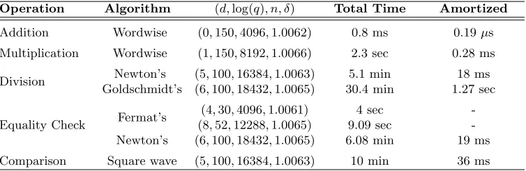
For 32 bit integer inputs, the parameters that are used in LTV setup can be seen in Table 1. For further details on selection of the security and noise parameters, we refer users to [8].
Binary Wordwise
Parameters + ∗ = < / + ∗ = < /
log(p) 1 1 1 1 1 32 32 20 20 20
d 6 10 5 6 96 − 1 6 5 5
log(q) 23 24 23 23 28 150 150 100 100 100
log(q0) 161 264 138 161 2716 150 300 700 600 600 n 8190 8190 8190 8190 131070 4096 8192 18432 16384 16384 δ 1.0033 1.0055 1.0028 1.0033 1.0035 1.0062 1.0066 1.0065 1.0063 1.0063
log(w) 3 3 3 3 3 − 30 25 25 25
#ζτ 20 33 17 20 339 − 10 28 24 24
#c(0) 64 64 64 64 64 2 2 ≈8 ≈16 ≈8
r 630 630 630 630 7710 4096 8192 18432 16384 16384
Table 1: Leveled DHS parameters for bit-wise and word-wise encryption. Key to parameters: log(p): bit size of the plaintext space; d: multiplicative depth of the circuit; log(q): bit size of the noise cutting factor; n: degree of the polynomial ring; δ: Hermite factor with respect to the maximum q and n; log(w): bit size of each relinearization block; #ζτ: number of relinearization blocks/evaluation keys for the first level; #c(0): number of total ciphertexts for two operands; r: number of message slots in case of batching enabled.
7 Implementation Results
withµ= 5 and inputs in the range [0,64], we used the RNS method with 4 different 20-bitpvalues, because p needs to be larger than 2(k−1)(2µ−1) = 280. In this test, we have a total execution time (including ring operations and relinearizations) of 5.1 minutes. Next, we evaluated Goldschmidt’s division by convergence algorithm forη = 5 and inputs in the range [0,64], in this case we used 20 different 20-bit p values, because p must be larger than 2`(2η+1−1) = 2378. We also evaluated the equality checks (and/or zero check) using both Fermat’s Little Theorem and division by Newton’s root finding method. We used two different setup (p, d) = (17,4) and (p, d) = (257,8) and disabled batching for this test. For the last test, we computed a comparison with inputs in the range [0,32] and α = 5, β = 16. In order to have p > 2`(2β−1) = 2155, we set 8 different 20-bitp values. Total
execution times can be seen in Table 2.
Operation Algorithm (d,log(q), n, δ) Total Time Amortized
Addition Wordwise (0,150,4096,1.0062) 0.8 ms 0.19µs Multiplication Wordwise (1,150,8192,1.0066) 2.3 sec 0.28 ms
Division Newton’s (5,100,16384,1.0063) 5.1 min 18 ms Goldschmidt’s (6,100,18432,1.0065) 30.4 min 1.27 sec
Equality Check Fermat’s
(4,30,4096,1.0061) 4 sec -(8,52,12288,1.0065) 9.09 sec -Newton’s (6,100,18432,1.0065) 6.08 min 19 ms Comparison Square wave (5,100,16384,1.0063) 10 min 36 ms
Table 2: Parameters and timings for: Zero Test using Fermat’s Little Theorem with a single message; Division first using root finding, then convergence algorithm for multiple packed data; Comparisonusing Square Wave approximation for multiple packed data.
8 Conclusion
This paper explores advances in word-based homomorphic encryption. Directly addressing the weakest points of the current word-based approach, we propose an assortment of solutions to chal-lenging algorithmic bottlenecks that have hampered existing systems from exploiting the full utility of ring operations in large characteristic. As our starting point, we have proposed three distinct approaches to inversion. These lead to efficient algorithms for division, zero test, equality check, thresholding, comparison, and square root, mostly in terms of approximation-based algorithms. We also introduce an extremely efficient technique for constant division and bring in the Chinese Remainder Theorem as a tool to improve the scalability of the proposed approximation algorithms. While many of these operations involve unsurprisingly high degree polynomials (hence require eval-uation of deep circuits), our implementation experiments give impressive amortized timings when batching is employed. The most practical use of these techniques remains in applications where all but a small number of gates are addition and multiplication gates, with approximation based algorithms applied only just before decryption.
References
1. Bos, J.W., Lauter, K., Loftus, J., Naehrig, M.: Improved security for a ring-based fully homomorphic encryption scheme. In: Stam, M. (ed.) Cryptography and Coding, Lecture Notes in Computer Science, vol. 8308, pp. 45–64. Springer Berlin Heidelberg (2013)
2. Bos, J.W., Lauter, K., Naehrig, M.: Private predictive analysis on encrypted medical data. Journal of biomedical informatics 50, 234–243 (2014)
3. Brakerski, Z.: Fully homomorphic encryption without modulus switching from classical gapSVP. IACR Cryptol-ogy ePrint Archive 2012, 78 (2012)
4. Brakerski, Z., Gentry, C., Vaikuntanathan, V.: Fully homomorphic encryption without bootstrapping. Electronic Colloquium on Computational Complexity (ECCC) 18, 111 (2011)
5. Brakerski, Z., Vaikuntanathan, V.: Efficient fully homomorphic encryption from (standard) LWE. In: Ostrovsky, R. (ed.) FOCS. pp. 97–106. IEEE (2011)
6. C¸ etin, G.S., Dor¨oz, Y., Sunar, B., Sava¸s, E.: Depth optimized efficient homomorphic sorting. In: Lauter, K., Rodr´ıguez-Henr´ıquez, F. (eds.) Progress in Cryptology – LATINCRYPT 2015, Lecture Notes in Computer Sci-ence, vol. 9230, pp. 61–80. Springer International Publishing (2015)
7. Cheon, J., Kim, M., Lauter, K.: Homomorphic computation of edit distance. In: Brenner, M., Christin, N., Johnson, B., Rohloff, K. (eds.) Financial Cryptography and Data Security, Lecture Notes in Computer Science, vol. 8976, pp. 194–212. Springer Berlin Heidelberg (2014)
8. Dor¨oz, Y., Hu, Y., Sunar, B.: Homomorphic AES evaluation using the modified LTV scheme. Designs, Codes and Cryptography pp. 1–26 (2015)
9. Gentry, C.: A Fully Homomorphic Encryption Scheme. Ph.D. thesis, Stanford University (2009)
10. Gentry, C.: Fully homomorphic encryption using ideal lattices. In: Proceedings of the Forty-first Annual ACM Symposium on Theory of Computing. pp. 169–178. STOC ’09, ACM (2009)
11. Gentry, C., Halevi, S.: Implementing Gentry’s fully-homomorphic encryption scheme. In: Paterson, K.G. (ed.) Ad-vances in Cryptology–EUROCRYPT 2011. Lecture Notes in Computer Science, vol. 6632, pp. 129–148. Springer (2011)
12. Gentry, C., Halevi, S., Smart, N.P.: Fully homomorphic encryption with polylog overhead. IACR Cryptology ePrint Archive Report 2011/566 (2011),http://eprint.iacr.org/
13. Gentry, C., Halevi, S., Smart, N.P.: Homomorphic evaluation of the AES circuit. IACR Cryptology ePrint Archive 2012 (2012)
14. Graepel, T., Lauter, K., Naehrig, M.: Ml confidential: Machine learning on encrypted data. Cryptology ePrint Archive: Report 2012/323 (June 2012)
15. Lagendijk, R., Erkin, Z., Barni, M.: Encrypted signal processing for privacy protection: Conveying the utility of homomorphic encryption and multiparty computation. Signal Processing Magazine, IEEE 30(1), 82–105 (Jan 2013)
16. Lauter, K., L´opez-Alt, A., Naehrig, M.: Private computation on encrypted genomic data. In: Aranha, D.F., Menezes, A. (eds.) Progress in Cryptology - LATINCRYPT 2014, Lecture Notes in Computer Science, vol. 8895, pp. 3–27. Springer International Publishing (2015)
17. Lindner, R., Peikert, C.: Better key sizes (and attacks) for lwe-based encryption. In: CT-RSA. pp. 319–339 (2011) 18. L´opez-Alt, A., Naehrig., M.: Large integer plaintexts in ring-based fully homomorphic encryption. in preparation
(2014)
19. L´opez-Alt, A., Tromer, E., Vaikuntanathan, V.: On-the-fly multiparty computation on the cloud via multikey fully homomorphic encryption. In: Proceedings of the Forty-fourth Annual ACM Symposium on Theory of Computing. pp. 1219–1234. STOC ’12, ACM (2012)
20. Naehrig, M., Lauter, K., Vaikuntanathan, V.: Can homomorphic encryption be practical? In: Proceedings of the 3rd ACM Workshop on Cloud Computing Security Workshop. pp. 113–124. CCSW ’11, ACM (2011)
21. Rivest, R.L., Adleman, L., Dertouzos, M.L.: On data banks and privacy homomorphisms. Foundations of Secure Computation pp. 169–180 (1978)
22. Shoup, V.:http://www.shoup.net/ntl/, NTL: A Library for doing Number Theory
23. Smart, N.P., Vercauteren, F.: Fully homomorphic SIMD operations. IACR Cryptology ePrint Archive 2011, 133 (2011)
24. Stehl´e, D., Steinfeld, R.: Making NTRU as secure as worst-case problems over ideal lattices. In: Paterson, K.G. (ed.) Advances in Cryptology EUROCRYPT 2011, Lecture Notes in Computer Science, vol. 6632, pp. 27–47. Springer Berlin Heidelberg (2011)
Appendix
Proof of Lemma 5.
Remark 1. We note that cases 2ri ≡ 0 (mod d) become simpler in the case when distribution χ generates only polynomials with non-negative coefficients.
Proof. Setq =p`+ 1 and U = `2−1 so thatkuk∞≤U. Observe that d0 =q−p`˜ is the inverse of
dinZq and write m0 =d0m.
We begin by expanding f˜cand, where possible, reducing modulo q to find
˜
c=d0hs+d0pe+d0m= ˜pgf−1s+ ˜pe+d0m
f˜c= ˜pgs+ ˜pf e+ (pf0+ 1)d0m= ˜pgs+ ˜pf e+ ˜pf0m+d0m= ˜pu+d0m .
Next, we substitutem=dm˜+randd0=q−˜p`as above:f˜c= ˜pu+d0dm˜+d0r= ˜pu+ ˜m+(q−p`˜ )r= ˜
pu+ ˜m−p`r˜ inZq[x]. So we can write ˜
L.Decrypt(˜c) =df˜ccq mod ˜p=dpu˜ + ˜m−p`r˜ cqmod ˜p
That is, ˆm=dMcqmod ˜pwhereM(x) = ˜pu(x)+ ˜m(x)−˜p`r(x) with coefficientsMi = ˜pui+ ˜mi−p`r˜ i for 0≤i < n. We will consider various cases and compute dMicqmod ˜p in each case.
First we observe that, in all cases, −q < Mi < q/2. Since ui ≥ −U, ˜mi ≥0 and ri ≤d−1, we haveMi ≥ −˜pU−p`˜(d−1) =−˜pU−p`d˜ + ˜p`= ˜p(`−U)−(q−1)>−q sinceU < `by hypothesis. Likewise, ui ≤ U and ˜mi < p˜ give Mi < q/2. So the balanced reduction modulo q takes a very simple form:
dMicq=
(
Mi+q, ifMi ≤ −q/2;
Mi, if −q/2< Mi ≤q/2.
(1)
Case 1:ri= 0 : Here,Mi = ˜pui+ ˜mi >−˜pU >−q/2 so thatdMicq=Mi anddMicqmod ˜p= ˜mi. Case 2:deven, ri=d/2 : First note that Mi is close to our boundary−q/2:
Mi = ˜pui+ ˜mi− p`
2 = ˜pui+ ˜mi− q−1
2 .
If ui ≥0, we obtain−q/2 < Mi < q/2 and dMicq =Mi. Since dis even, 2˜p dividesq−1 and we have dMicq mod ˜p= ˜mi. On the other hand, ifui <0, ˜mi <p˜gives ˜pui+ ˜mi<0 and Mi<−q/2 so that dMicq=Mi+q and
dMicqmod ˜p=
˜
pui+ ˜mi− p`
2 +p`+ 1
mod ˜p= ˜mi+ 1.
This dependence on ui is reflected in the statement of the theorem by replacingri by ri−ui/2U.
Case 3: 0 < ri < d/2 : Since U < 2` and d ≥ 2, ˜pU + ˜p`bd−21c < q2 and ˜pU + ˜p`ri < q2, thus Mi= ˜pui+ ˜mi−p`r˜ i >−q2 .So dMicq=Mi anddMicqmod ˜p= ˜mi in this case.