ABSTRACT
WHITE, KYLE ROSS. Model-Agnostic Variable Selection Through Measurement Error Model Selection Likelihoods. (Under the direction of Leonard A. Stefanski and Yichao Wu.)
A new wrapper method of variable selection is developed that can be applied to any “black-box” prediction model without the requirement of a likelihood. We first establish a connection between measurement error attenuation and L1- and L2-penalized linear regression by showing that weak model features may be viewed as contaminated with measurement error. Then, we force “false” measurement error into a fitting procedure and optimize the distribution of the errors across the predictors such that in-sample black-box predictions are impacted the least. The least important variables will absorb the most error. Using an inverse measurement error variance parameterization, we achieve variable selection by allowing features to absorb an infinite amount of error. We call this approach Measurement Error Model Selection Likelihoods, MEMSEL.
We define a four-step outline to MEMSEL and demonstrate it in the familiar context of linear regression. We prove the equivalence between MEMSEL and LASSO in the linear model. Thus, MEMSEL is a penalty-free generalization of LASSO. We apply it to the problem of variable selection in nonparametric classification, resulting in a new kernel-based classifier with LASSO-like variable shrinkage and selection properties. Finite-sample performance of the new classification method is studied via simulation and real-data examples, and consistency of the method is studied theoretically.
explored via Monte Carlo experiments and applications to data.
© Copyright 2017 by Kyle Ross White
Model-Agnostic Variable Selection Through Measurement Error Model Selection Likelihoods
by
Kyle Ross White
A dissertation submitted to the Graduate Faculty of North Carolina State University
in partial fulfillment of the requirements for the Degree of
Doctor of Philosophy
Statistics
Raleigh, North Carolina 2017
APPROVED BY:
Dennis Boos Eric Laber
Leonard A. Stefanski Co-chair of Advisory Committee
Yichao Wu
DEDICATION
BIOGRAPHY
ACKNOWLEDGEMENTS
First and foremost, thank you Dr. Stefanski. I will never forget the day in January 2012 that you convinced me to cancel my job search and stick with research. Thank you for the opportunity to work on this project with you. Thank you for believing in me and always being a source of encouragement and motivation.
To both of my advisors, Dr. Stefanski and Dr. Wu, thank you for your wisdom, guidance, and endless patience. I truly appreciate all of time you spent with me on this research and as mentors. Thank you for all the thoughtful discussions and comments that greatly improved my work. And I cannot thank you enough for the flexibility to allow me to balance research with my career and personal life.
To Dr. Boos, Dr. Laber, and Dr. Healey, thank you for serving on my committee and providing feedback on this dissertation.
To Dr. Davidian and Dr. Wu, thank you for funding me through portions of your grants (NIH T32HL079896; NIH P01CA142538; NSF DMS-1055210).
To the DCRI, thank you for the internship opportunity and invaluable experience. Special thanks to Karen Pieper for her incredibly selfless mentorship.
To Republic Wireless, thank you for giving me the freedom to finish this dissertation. To The Fifth Moment, thank you for all of the memorable performances (and practices). To my first-year cohort, thank you for making my transition to Raleigh easy and for the lifelong friendships. I was lucky to start at the same time as the rest of you.
To my closest friends—Joe and Jesse—thank you for your companionship and support, and for providing many welcome distractions.
To mom, dad, and bro, thank you for being there for me since day one.
TABLE OF CONTENTS
LIST OF TABLES . . . vii
LIST OF FIGURES . . . ix
Chapter 1 INTRODUCTION . . . 1
Chapter 2 MEASUREMENT ERROR MODEL SELECTION LIKELIHOODS 4 2.1 Introduction . . . 4
2.2 Variable Selection and Measurement Error . . . 6
2.2.1 Attenuation, Shrinkage, and Selection . . . 6
2.2.2 Oracle Heuristics . . . 8
2.2.3 MEM Selection Likelihoods . . . 9
2.3 Linear Model Selection Likelihoods . . . 11
2.3.1 Linear Regression . . . 11
2.3.2 Relationship to LASSO . . . 13
2.4 Nonparametric Classification . . . 15
2.4.1 Selection Likelihoods for Classification . . . 15
2.4.2 Multicategory SKDA . . . 18
2.4.3 Simulation Studies . . . 18
2.4.4 Illustrations with Real Data . . . 29
2.4.5 Consistency of SKDA . . . 32
2.5 Summary . . . 35
2.6 Appendix (Supplemental Files) . . . 36
2.6.1 Equivalence of LASSO andLbSEL1-MESSO . . . 36
2.6.2 Generating Sparse Classification Data . . . 45
2.6.3 Proofs of Asymptotic Results . . . 45
Chapter 3 MEKRO. . . 50
3.1 Introduction . . . 50
3.2 Measurement Error Kernel Regression Operator . . . 52
3.2.1 Example . . . 54
3.2.2 Tuning and Solution Paths . . . 55
3.3 Extension to Categorical Predictors . . . 57
3.4 Method Comparison and Numerical Results . . . 58
3.4.1 Simulation Preliminaries . . . 59
3.4.2 Simulation Results . . . 61
3.5 Asymptotic Results . . . 72
3.6 Discussion . . . 72
3.7 Appendix . . . 74
3.7.1 MEKRO Selection Likelihood Derivation . . . 74
3.7.2 Asymptotic Selection Consistency . . . 76
Chapter 4 GENERAL MEASUREMENT ERROR MODEL SELECTION
LIKE-LIHOODS . . . 82
4.1 Introduction . . . 82
4.2 Selection Information Criterion . . . 83
4.2.1 Comparing Tuning Criteria Penalties . . . 84
4.2.2 Tuning Method Simulation Study . . . 86
4.2.3 SIC Sensitivity Analysis top . . . 93
4.3 MEMSEL . . . 96
4.3.1 Contamination Via Pseudo-Measured Predictors . . . 97
4.3.2 MEMSEL Objective, Optimization, and Tuning . . . 100
4.4 MEMSEL in Linear Models . . . 102
4.4.1 Simulation Study Setup . . . 106
4.4.2 Simulation Study Results . . . 107
4.5 MEMSEL in Random Forests . . . 113
4.5.1 Motivation . . . 113
4.5.2 Selection Using Variable Importance . . . 113
4.5.3 Simulation Study Setup . . . 115
4.5.4 Software Considerations . . . 116
4.5.5 Simulation Study Results . . . 116
4.5.6 Real Data Example – Concrete Workability . . . 119
4.6 Summary . . . 121
4.7 Appendix . . . 122
4.7.1 Centering and ScalingZ . . . 122
4.7.2 Derivation of MEMSEL in Linear Models . . . 123
LIST OF TABLES
Table 2.1 Predictor selection frequencies for SKDA and SLDA for the study in Section 2.4.3.1. . . 20 Table 2.2 Predictor selection frequencies for SKDA and SLDA for the study in Section
2.4.3.2. . . 22 Table 2.3 Frequency ofX1 andX2 and the average frequency of X3, . . . , X50 being
selected by SKDA and SLDA. . . 25 Table 2.4 Predictor selection frequencies for MSKDA for the study in Section 2.4.3.3. 25 Table 2.5 Predictor selection frequencies for MSKDA for the study in Section 2.4.3.4. 28 Table 2.6 Test error summary for 40 random splits of the WBCD data. . . 29 Table 2.7 Predictor selection frequencies for SLDA and SKDA for the WBCD data
example. Asterisks indicate variables selected using the entire data set. . . 30 Table 2.8 Test error summary for 40 random splits of the chemical signature data. . 31 Table 2.9 Predictor selection frequencies for SLDA and SKDA for the chemical
signature data. Asterisks indicate variables selected using the entire data set. 33 Table 3.1 Selection error rates for Model 1. MC standard errors for all cells≤0.03. . 62 Table 3.2 Selection error rates for Model 2. MC standard errors for all cells≤0.03. . 64 Table 3.3 Selection error rates for Model 3. MC standard errors for all cells≤0.03. . 66 Table 3.4 Selection error rates for Model 4, withX1inZ(·) andX4classified irrelevant.
MC standard errors for all cells≤0.04. . . 67 Table 3.5 Main effect selection rates (not errors) for Model 5, averaged over the
four simulation settings. The IRR row is the average selection rate for the four irrelevant predictors that were independently generated. MC standard errors for all cells ≤0.03. . . 69 Table 3.6 Main effect selection rates (not errors) for the prostate data. ‘Avg Model’
is the method’s average model size; ‘Corr’ is the selection rate correlation of each method with LAS. MC standard errors for all selection rates≤0.07 and all average model sizes≤0.55. . . 70 Table 3.7 Selection error rates for the model in Appendix C. MC standard errors for
all cells≤0.03. . . 81 Table 4.1 Simulation setup to study effects of n, p, p1 on SIC. Both p and n are
explicitly chosen as simulation factors. The number of non-zero coefficients p1 is implied by the choice of β and r. There are 84 total simulations created from full crosses ofr,p, and nin each row. . . 93 Table 4.2 Selection and prediction errors for random forest MEMSEL (XM1, XM2),
LIST OF FIGURES
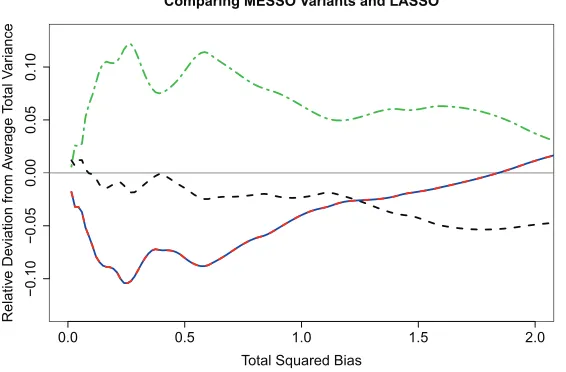
Figure 2.1 Plot of relative deviations from the average total variance versus total squared bias. LASSO (red-dashed); MESSO estimator from LbSEL1 (solid
blue); full-conditional MESSO estimator from LbSEL1LbSEL2 (black dashed);
and the full-unconditional MESSO estimator from LbSEL1LbSEL2LbSEL3 (green
dot-dash). Because of their equivalency the LbSEL1-MESSO and LASSO
lines overlap and appear as a single alternating red/blue dashed line. . . 13 Figure 2.2 Plots of typical training samples and boxplots of test errors for data
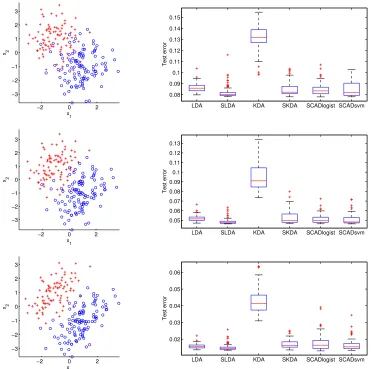
generated with ρ= 0 (top), 0.3 (middle), and 0.6 (bottom), from Section 2.4.3.1. . . 21 Figure 2.3 Plot of one training sample (left) and boxplots of test errors (right) for
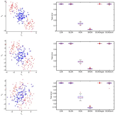
the study in Section 2.4.3.2 with p= 10 and three values ofρ: 0 (top), 0.3 (middle), and 0.6 (bottom). . . 23 Figure 2.4 Plot of one training sample (left) and boxplots of test errors (right) for
the study in Section 2.4.3.2 with p= 50 and three values ofρ: 0 (top), 0.3 (middle), and 0.6 (bottom). . . 24 Figure 2.5 Plot of one training sample (left) and boxplots of test errors (right) for
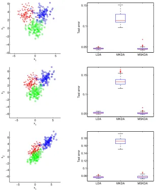
the study in Section 2.4.3.3. . . 26 Figure 2.6 Plot of a training sample (left) and boxplots of test errors (right) for the
discrete predictor simulation study in Section 2.4.3.3. . . 27 Figure 2.7 Plot of one training sample (left) and boxplots of test errors (right) for
the study in Section 2.4.3.4. . . 28 Figure 2.8 Boxplots of test errors for the WBCD example . . . 30 Figure 2.9 Chemical data heat map. First 50 columns (left to right) are the “Y = 0”
group. Columns within groups randomly ordered. Rows identify compounds X1, . . . , X38. . . 32 Figure 3.1 LbSEL(λ) contours and gradient vector fields of example model (3.5) for
λ = (λ1, λ2, λ3 = τ −λ1 −λ2) and τ ∈ {1,2,3}; global maxima are denoted with solid circles and the neutral starting values λstart = (τ /p)1p are denoted with solid diamonds. . . 55 Figure 3.2 Solution paths of bλτ versusτ for Section 3.2.1 example with two active
(solid) and three irrelevant (open) predictors. Dashed line: scaled AICc(τ),
τ ∈τ∗ ={0,0.5, . . . ,7}. . . 56 Figure 3.3 AISEs for Model 1. Note the scale differences. Out of the 400 MC samples,
3 AISE outliers are omitted from M3. . . 62 Figure 3.4 Study of AMKR estimates for Model 1, n= 400. . . 63 Figure 3.5 AISEs for Model 2. Note the scale differences. Out of the 400 MC samples,
19 and 6 AISE outliers are omitted from M3 and M2, respectively. . . 64 Figure 3.6 AISEs for Model 3. Note the scale differences. Out of the 400 MC samples,
Figure 3.7 AISEs for Model 4; units for Z(·) plots are 103 and units for φ(·) plots are 10−3. Note the scale differences. Dashed lines indicate methods with AISEs too large to display. . . 67 Figure 3.8 ASPEs (average squared prediction errors) for Model 5. Note the scale
differences. Out of the 400 MC samples, 3 ASPE outliers are omitted from both M3 and M2. . . 69 Figure 3.9 ASPEs (average squared prediction errors) for the prostate data. Out of
the 100 MC samples, 2 and 4 ASPE outliers are omitted from M3 and M2, respectively. . . 71 Figure 3.10 AISEs (average integrated squared errors) for Appendix C Model. Note
the scale differences. Out of the 400 MC samples, 2 AISE outliers are omitted from both M2 and M3. . . 81 Figure 4.1 Comparing overfitting penalties in AIC (dashed line), BIC (solid line),
GCV (dash-dot-dash line), and SIC (dotted lines) as model degrees of freedom (k) increase. Left pane: n = 50. Right pane: n = 100. Larger penalties for the same model degrees of freedom result in sparser models. 85 Figure 4.2 Comparison of perfection selection rates (higher is better). 100 MC
repli-cates are used for each model. Paired t-tests of SIC versus other methods are displayed in teal if statistically different from SIC and red otherwise atα = 0.05. . . 90 Figure 4.3 Comparison of perfection rates with increased n (higher is better). 100
MC replicates are used for each model. Paired t-tests of SIC versus other methods are displayed in teal if statistically different from SIC and red otherwise at α= 0.05. . . 91 Figure 4.4 Comparison of test errors in SIC simulation study (lower is better). 100
MC replicates are used for each model. Paired t-tests of SIC versus other methods are displayed in teal if statistically different from SIC and red otherwise at α= 0.05. . . 92 Figure 4.5 Results of sensitivity analysis of SIC. Each of the 84 points coincides with
one simulation described in Table 4.1. Results are the tuning method that had the best perfect selection rate over 100 MC replicates. The results “best,” “tied,” and “not best” are judged with a paired t-test atα= 0.05. 95 Figure 4.6 Comparing AIC curves against coefficient size between LASSO (gray
solid line) and the equivalent MEMSEL variant, (W,W) with m = 1 (red dashed line). Left: a grid size of 10 is used in MEMSEL modified coordinate descent. Right: a grid size of 100 is used in MEMSEL modified coordinate descent. Identical data are used for both plots. Discrepancies occur when optimizedλbτ values are not global minimizers. The gray (red)
circle denotes the minimum AIC value for LASSO (MEMSEL). . . 108 Figure 4.7 Results from linear Model 1. Estimation methods are along the horizontal
Figure 4.8 Results from linear Model 2. Estimation methods are along the horizontal axis and selection errors and test loss are along the vertical axis separated by panes. Tuning methods are grouped within fitting method and show a 95% confidence interval. Note the test loss axis is truncated. . . 111 Figure 4.9 Results from linear Model 3. Estimation methods are along the horizontal
axis and selection errors and test loss are along the vertical axis separated by panes. Tuning methods are grouped within fitting method and show a 95% confidence interval. Note the active selection error and test loss axes are truncated. . . 112 Figure 4.10 Distribution of RMSEs from concrete data. The thin solid vertical line
CHAPTER
1
INTRODUCTION
We study an algorithm to achieve variable selection generally, agnostic to the choice of model describing observed data. A common approach to variable selection adds an L1-penalty term to the likelihood to encourage coefficient sparsity. This is not straightforward or even sensible on complex models or models without coefficients or a likelihood. We propose a “wrapper method” variable selection approach to apply to any black-box method that produces a prediction function from input data. The idea is closely related to the coefficient attenuation observed when predictors are contaminated with measurement error, coining this approach broadly as Measurement Error Model Selection Likelihoods (MEMSEL). The acronym MEMSEL may be used to describe either the proposed variable selection method or the selection likelihood itself.
• Chapter 2. Taken verbatim (with minor stylistic edits) from [68],
Stefanski, L. A. et al. “Variable Selection in Nonparametric Classification Via Measurement
Error Model Selection Likelihoods.” Journal of the American Statistical Association
109.506 (2014), pp. 574-589.
This chapter describes the relationship between measurement error and variable selection. It outlines a four-step approach for building measurement error selection likelihoods and proves the equivalence between (one variant of) MEMSEL in the linear model and LASSO. MEMSEL is applied to kernel-based discriminant analysis to produce Sparse Kernel Discriminant Analysis (SKDA) that demonstrates favorable performance over other sparse classifiers. Two real-data examples regarding breast cancer and gas well classification are given. Selection consistency for the MEMSEL classifier is proved.
• Chapter 3. Taken verbatim (with minor stylistic edits) from [79],
White, K. R. et al. “Variable Selection in Kernel Regression Using Measurement Error
Selection Likelihoods.” Journal of the American Statistical Association (accepted, to
appear).
This chapter extends the work from Chapter 2 and applies MEMSEL to kernel density-based regression. The result is the Measurement Error Kernel Regression Operator (MEKRO). It has the same form as the Nadaraya-Watson estimator [53, 78] but with smoothing parameters determined by the MEMSEL variable selection algorithm. A method of handling categorical input variables is defined. Simulations demonstrate that MEKRO has superior selection and predictive performance to other selection-capable nonparametric regression approaches on models with many interactions. Real-data examples on robot arm movement and prostate cancer are provided. An argument for selection consistency is given.
for selection. The four-step method from Chapter 2 is then generalized to include different forms of predictor contamination. As an aid to understanding how the new approach works, general MEMSEL variants are applied to linear models in detail via theory and simulation. A subset of general MEMSEL variants coupled with a random forest black-box estimator are then compared to other random forest selection estimators. MEMSEL shows favorable selection and prediction results. Random forest MEMSEL is illustrated on a real data set regarding wet concrete workability.
CHAPTER
2
MEASUREMENT ERROR MODEL
SELECTION LIKELIHOODS
2.1
Introduction
Adopting a measurement-error-model-based approach to variable selection, we propose a non-parametric, kernel-based classifier with LASSO-like shrinkage and variable-selection properties. The use of measurement error model (MEM) ideas to implement variable selection is new and provides a different way of thinking about variable selection, with potential for applications in other nonparametric variable selection problems. Thus we also describe what we call mea-surement error selection likelihoods in addition to our main methodological results on variable selection in nonparametric classification.
methods is in its infancy. Our research helps fill that gap with a sparsity-seeking kernel method,
sparse kernel discriminant analysis (SKDA), obtained by implementing the MEM-based ap-proach to variable selection. SKDA is kernel-based with a familiar form, but with a bandwidth parameterization and selection strategy that results in variable selection. We provide additional background and introductory material at the start of the main methodological section on classification, Section 2.4.
In response to a suggestion by the Associate Editor we end this section with remarks relating to the potential benefits of approaching variable selection problems via measurement error models. The fact that a version of our MEM-based approach to variable selection applied to linear regression results in LASSO estimation is of independent interest. Knowing different paths to the same result and the relationships among them, enhances understanding even when it does not lead to new methods. However, our approach is more than just another LASSO computational algorithm. It is a useful conceptualization and generalization of the LASSO that has potential to suggest new variable selection methods.
Penalizing parameters is not always intuitive simply because it is not always the case that variables enter a model through easily intuited parameters; as with nonparametric models and algorithmic fitting methods. However, it is always possible to intuit the case that a variable has (a lot of) measurement error in it. Admittedly, turning the idea that a variable contains measurement error into a variable selection method may require additional, creative modeling, and perhaps extensive computing power to simulate the measurement error process when analytical expressions are not possible. However, the key point is that the MEM-based approach provides another way for researchers to think about variable selection in nonstandard problems. Although variable selection in nonparametric classification is the primary methodological contribution of the paper, the idea of approaching variable selection via measurement error modeling may have broader impact because of the possibility of adapting the strategy to other problems not readily handled by traditional penalty approaches.
the new approach to variable selection are discussed in Section 2.2. The new approach is illustrated in the context of linear regression in Section 2.3. The main results on variable selection in nonparametric classification are in Section 2.4, which includes performance assessment via simulation studies, applications to two data sets, and asymptotic results. Concluding remarks appear in Section 2.5 and technical details in the online supplemental materials.
2.2
Variable Selection and Measurement Error
We now describe the connection between measurement error and variable selection that is used to derive the nonparametric classification selection method studied in Section 2.4.
2.2.1 Attenuation, Shrinkage, and Selection
We begin with the connections between measurement error attenuation, ridge regression, and LASSO estimation in linear models Yn×1 =Xβp×1+.
Measurement error attenuation.Measurement error attenuation is usually introduced in the case of simple linear regression in terms of ‘true’ {Yi, Xi}, and measured{Yi, Wi} data,
i= 1, . . . , n, where Wi =Xi+σUZi, andZi iid
∼ N(0,1) with theZi independent of (Xi, Yi) [8, 11, 24]. The least squares slope ofY onW, βbATTEN =syw/s2w
p
−→σyw/σ2w= σx2+σ2U
−1
σyx. Attenuation results from the inequality σx2+σU2 > σ
2
x. The multi-predictor version of this result for the error model W =X+D{σ
U}Z, with D{σU} = diag(σU,1, . . . , σU,p) and Z∼ N(0, I) is
b
βATTEN=Vb −1
W VbWY ≈
b
VX +D
σ2U
−1 b
VXY =
b
VX +D−1
1/σ2 U
−1 b
VXY. (2.1)
Notes. i) The approximation “≈” in (2.1) is valid in large samples because Vb
−1
W VbWY −
b
VX+D
σ2U
−1 b
VXY converges in probability to0. ii)We use 1/σ2U to denote componentwise division, i.e., 1/σ2U = (1/σ
2
U,1, . . . ,1/σ 2 U,p)
(or square-root precisions). iv) We use D{v} to denote a diagonal matrix with vector v on its diagonal. v) For any vector z, |z| denotes the vector of componentwise absolute values. Similarly,zm denotes the vector of componentwisemth powers.vi) Finally,Vb denotes a sample
variance/covariance matrix of the subscripted variables.
Ridge shrinkage.Ridge regression [38] is much studied and well known. Thus we simply note that after scaling the ridge parameters ν it has the form
b
βRIDGE =
b
VX+D{ν}
−1 b
VXY =
b
VX +D−1{1/ν} −1
b
VXY. (2.2)
LASSO shrinkage and selection. The LASSO has an attenuation-like representation that follows from the iterated-ridge computation algorithm; see [74] and Section 2.3.2. The iterated ridge solution to the penalty form of the LASSO optimization is
b
βLASSO = argmin
β1,...,βp
1
n−1kY −Xβk 2+η
p
X
j=1 |βj|
(2.3)
= I +Dn
|βbLASSO|/η
oVbX !−1
Dn
|βbLASSO|/η
oVbXY (2.4)
= VbX +D−1n
|βbLASSO|/η o
!−1 b
VXY. (2.5)
Notes: i)Expressions (2.4) and (2.5) are not computational solutions to the LASSO optimization problem, but rather equations satisfied by the solution.ii)Both are included to show that the inversion of a singular matrix in (2.5) when some components ofβbLASSO are zero is not necessary;
however, we use expressions like that in (2.5) for their compactness.
the sameformof attenuation, with equality in the case that
1 σ2 U,j
= 1 νj
= |βbLASSO,j|
η .
Measurement error attenuation results from uncontrollable and undesirable measurement error in the predictors, whereas ridge and LASSO attenuation is analyst-controlled to manipulate sam-pling properties of the estimators. In Section 2.2.3 we show that measurement error attenuation can also be controlled to accomplish shrinkage and selection. For another interesting example of creatively using measurement error to impart favorable sampling properties on estimators in a different context, see [62].
2.2.2 Oracle Heuristics
We motivate our measurement error approach to variable selection using a toy example, imagining an oracle’s solution to a simple challenge. Suppose that the regression of Y on predictors X1, . . . , X5 satisfies
E(Y |X1, X2, X3, X4, X5) =E(Y |X2, X5).
The nullity ofX1, X3, and X4 is unknown to a statistician, but not to the oracle. However, sup-pose the oracle agrees to play a game wherein s/he must add a nonzero, total amount of measure-ment error, (σU,1Z1, σU,2Z2, σU,3Z3, σU,4Z4, σU,5Z5), to the predictors (X1, X2, X3, X4, X5) in a manner that minimizes the loss of their collective predictive power (“a nonzero, total amount of measurement error” means thatP
jσU,2j >0).
Because the oracle knows that
E(Y |X1, X2, X3, X4, X5) =E(Y |X2, X5) =⇒
the oracle’s solution is to setσU,2=σU,5= 0 and letσU,1, σU,3, andσU,4be nonzero. A statistician seeing the oracle’s solution would know the identity of the null and informative predictors. In the next section we show that this oracle game can be mimicked using a (pseudo-profile) likelihood to replace the omniscience of the oracle, and constraints to ‘force’ the addition of measurement error to the data.
2.2.3 MEM Selection Likelihoods
We now give a general description of the construction and use of measurement error model (MEM) selection likelihoods. As an illustration of the approach, we then implement it for linear models in Section 2.3, where it is shown to lead to the LASSO for linear models. This equivalency lends credibility to the new approach in the sense that it can be viewed as a generalization of the LASSO that reduces to the LASSO in the case of linear regression. In Section 2.4 we implement the approach in the context of nonparametric classification obtaining the new method,sparse kernel discriminant analysis (SKDA). The latter is the main methodological contribution of the paper. However, Section 2.4 also demonstrates the utility of the measurement error approach to variable selection for identifying and deriving variable selection strategies in nonparametric/nonstandard models.
Denote the data as (Yi, Xi), i= 1, . . . n, and let (Y, X) represent a generic observation. The MEM selection likelihood construction proceeds in four basic steps:
1. Start with an assumed ‘true’ likelihood for (Xi, Yi), i = 1, . . . , n, denoted LTRUE(θ) where θ could be finite (parametric) or infinite dimensional (nonparametric).
2. Construct the associated MEM likelihood under the ‘false’ assumption that the components ofX are measured with independent error. That is, assume that W is observed in place of X whereW |X ∼ NX, D
σ2 U
with σ2U= σ 2
U,1, . . . , σ 2 U,p
. The resulting likelihood depends onθ andσ2
U and is denotedLMEM(θ,σ 2
3. Replaceθ inLMEM(θ,σ2U) with an estimatebθ, resulting in the pseudo-profile likelihood
b
LpMEM(σ2U) =LMEM(θb,σ 2
U). Note thatbθis an estimator forθ calculated from the observed data without regard to the ‘false’ measurement error assumption, e.g., bθ could be the
maximum likelihood estimator fromLTRUE(θ).
4. Reexpress the pseudo-profile likelihood LbpMEM(σ2U) in terms of precision (or square-root
precision) λ = (λ1, . . . , λp) where λj = 1/σU,2j (or λj = 1/σU,j), resulting in the MEM
selection likelihoodLbSEL(λ).
b
LSEL(λ) is maximized subject to: λj ≥ 0, j = 1, . . . , p; and Pjλj ≤ τ. Setting the tuning parameterτ <∞ in the latter constraint ensures that the harmonic mean of the measurement error variances (or standard deviations) is ≥ p/τ > 0. This is how the approach ‘forces’ measurement error into the likelihood. Maximizing LbSEL(λ) subject to the constraint ensures
that the measurement error is distributed to predictors optimally in the sense of diminishing the likelihood the least. The idea is that null predictors tend to be assigned large measurement error variances, whereas informative predictors tend to be assigned relatively small ones. Thus maximizing LbSEL(λ) plays the role of the oracle. The constrained maximum can have some b
λj = 0 for small τ, indicating that the data are consistent with predictorXj containing infinite measurement error, and therefore is uninformative. Note thatbλj = 0 =⇒ bσ2U,j= 1/0 =∞, see
(2.6).
Standardization was not mentioned previously. Doing so facilitates interpretation, numerical calculation, and comparison with other estimators, thus we assume henceforth that predictor variables are centered and scaled to unit variance. Viewed from the measurement error perspective, standardization ensures that the measurement error variances referred to in the development in Section 3,σ2U,1, . . . , σ
2
U,p, are all on the same scale.
familiar context of linear regression, which also serves to justify the approach since we show it leads to the LASSO. In Section 2.4 we show that the approach leads to a useful new variable selection method for kernel-based classification rules.
2.3
Linear Model Selection Likelihoods
2.3.1 Linear Regression
We start with the assumption that (Y, X) is multivariate normal with mean µY, µXT T
and partitioned variance matrix VY,VXTY,VXY,VX
. Under the ‘false’ assumption that the predictor is measured with error, the distribution is multivariate normal with the same mean, but with partitioned variance matrix
VY,VXTY,VXY,VX+D
σ2 U
. Thus
LTRUE(θ) = Y i
ΨYi,Xi; µY, µXT T
, VY,VXTY,VXY,VX
,
LMEM(θ,σ2U) =
Y
i
ΨYi,Xi; µY, µXT T
,VY,VXTY,VXY,VX+D
σ2U
,
where Ψ(y,x;µ,Ω) is the multivariate normal density with meanµand variance matrix Ω, and θ = (µY,µX, VY,VXY,vech(VX)). We set bθ equal to the sample moments of (Yi, Xi), i=
1, . . . n, i.e., bθ=
b
µY, µbX, VXY, VbXY, vech(VbX)
. Then with βb(λ) =
b
VX +D{−1λm} −1
b
VXY, where λm = λm1 , . . . , λmp
, and m = 1 for λj = 1/σ2U,j and m= 2 for λj = 1/σU,j, it follows that
b
where
b
LSEL1 =
n b
VY −VbXTYβ(λ)b o−n/2
,
b
LSEL2 = exp
− n 2 b
VY −VbXTYβ(λ) +b n
b
β(λ)TVbXβ(λ)b −VbXTYβ(λ)b o
b
VY −VbXTYβ(λ)b
,
b
LSEL3 =
det
b
VX+D{−1λm}
−1n/2
exp −n 2tr b VX b
VX +D−1{λm}
−1
. (2.6)
FactoringLbSEL as in (2.6) facilitates discussion of the linear model in Section 2.3.2. Although
b
VX +D−1{λm} −1
is more succinct, when a component of λ is 0, we use either of the equivalent expressions,
I+D{λm}VbX −1
D{λm} or D{λm}
I+VbXD{λm} −1
(compare to (2.4) and (2.5)). These identities imply that
b
β(λ) =
b
VX+D{−1λm}
−1 b
VXY =D{λm}
I+VbXD{λm} −1
b
VXY =I+D{λm}VbX
−1
D{λm}VbXY, (2.7)
from which it is apparent that λj = 0 implies that the jth component of βb(λ) = 0. The
simple identity D{v
1}v2 = D{v2}v1 shows that βb(λ) = D{∆}λ
m where ∆ = ∆(λ) =
I+VbXD{λm} −1
b
VXY. Under common distributional assumptions onY1, . . . , Yn, the compo-nents of∆are nonzero almost surely. In this case it follows thatλm=D−1{
∆}βb(λ) almost surely,
and thus thejth component of βb(λ) = 0 if and only if λj = 0.
We now study MEM selection likelihood method for linear regression in the case thatλj is parameterized in terms of precisions (m= 1). The main results in the following section are: i) maximizingLbSEL1 is a convex optimization problem that yields an estimator equivalent to the
LASSO; ii) maximizing the full-conditional likelihoodLbSEL1LbSEL2 with m= 1 is not equivalent
to the LASSO, and in terms of variance per shrinking bias, can be less variable than the LASSO; and iii) maximizing the full likelihoodLbSEL1LbSEL2LbSEL3 can never result in bλj = 0 and thus is
MESSO (Measurement Error Shrinkage and Selection Operator) to identify estimators derived from the selection likelihoods in Section 2.3.1.
2.3.2 Relationship to LASSO
In the supplemental Appendix Section 2.6.1 we prove that constrained maximization of LbSEL1
in (2.6) results in LASSO solution paths as functions of τ. The proof establishes convexity of bσ2(λ) =
b
LSEL1
−2/n
and equivalence of KKT conditions. Note that although the MESSO selection likelihood in Section 2.3 was derived starting with an assumption of multivariate normality, the equivalency to the LASSO does not depend on that assumption.
We now consider the relationship of LASSO to other MESSO versions obtained by maximizing the full-conditional likelihood,LbSEL1LbSEL2, and the full likelihoodLbSEL1LbSEL2LbSEL3 forλj = 1/σj2
andλj = 1/σj. A detailed comparison is beyond the scope of this paper. However, we make a
0.0 0.5 1.0 1.5 2.0
−0.10
−0.05
0.00
0.05
0.10
Comparing MESSO Variants and LASSO
Total Squared Bias
Relativ
e De
viation from
A
v
er
age T
otal V
ar
iance
Figure 2.1 Plot of relative deviations from the average total variance versus total squared bias.
LASSO (red-dashed); MESSO estimator fromLbSEL1 (solid blue); full-conditional MESSO estimator
fromLbSEL1LbSEL2 (black dashed); and the full-unconditional MESSO estimator fromLbSEL1LbSEL2LbSEL3
(green dot-dash). Because of their equivalency the LbSEL1-MESSO and LASSO lines overlap and appear
few brief, relevant observations. Figure 2.1 displays plots of relative deviations from average total prediction error variance versus total squared prediction error bias from a small simulation study comparing LASSO and the three MESSO estimators when λj = 1/σ2j. That is, the plot displays {TV-Ave(TV)}/Ave(TV) versus TB, where: TB={Eb(β)b −β}TΩ{Eb(β)b −β};
TV=tr{Var(d β)Ω};b Ω is the predictor covariance matrix; Ave(TV) is TV averaged over the
three unique estimators; andEb andVar denote Monte Carlo expectation and variance. The plotd
allows differentiation of the estimators based on total variance for equivalent total squared bias. Data were simulated according to a design in [74]: Yi =XTi β+σi,i= 1, . . . , n, where Xi are iidN(0p×1, AR1(ρ)), i are iidN(0, 1), with n= 20,p= 8,β= (3,1.5,0,0,2,0,0,0)T, ρ=.5, and σ = 3. This model calls for a mix of selection and shrinkage. Figure 2.1 shows that the LASSO is less variable (as measured by tr{Var(d β)Ω}) for small total squared bias (as measuredb
by {Eb(β)b −β}TΩ{Eb(β)b −β}), but not for larger values of TB. For reference, we obtained
TB=1.27 for the LASSO estimator tuned using 10-fold cross validation, which corresponds very closely to the value of TB for which the black-dashed and red-blue curves intersect. Thus in a region of total squared bias of known practical importance, the LASSO and the full-conditional MESSO estimator have similar total variance.
Examination of LbSEL3 in (2.6) reveals that if any λj = 0, then the determinant term is
zero and the maximizer of the full likelihood LbSEL1LbSEL2LbSEL3 never contains zero elements, i.e.,
selection is not possible. Finally, when λis parameterized as square-root precisions, λj = 1/σj, the MESSO optimization is no longer convex, and results in greater selection.
Our comparison to the LASSO is not because we consider MESSO to be a competitor to the LASSO for linear models, but rather to establish the viability of the new approach in a familiar context. In the next section we show that it leads
2.4
Nonparametric Classification
Classification has a long and important history in statistics. Several methods are widely used: Fisher’s linear discriminant analysis [LDA, 19]; logistic regression [52]; support vector machine [13, 76]; and boosting [20]. LDA is the estimated Bayes rule under within-class normality and equal covariance matrices [3], whereas with unequal covariances the estimated Bayes rule is quadratic discriminant analysis (QDA).
A nonparametric Bayes rule obtained by replacing conditional densities in the theoretical Bayes rule with kernel density estimates [77] is known as kernel density-based discriminant analysis (KDA) [12, 27]. See [14] and [36] for recent reviews of KDA.
With multiple predictors, variable selection is important. Some predictors may not carry useful information and their inclusion can deteriorate performance of an estimated classification rule. [6] studied how dimension affects performance and showed that LDA behaves like random guessing when the ratio of pto n is large. Thus motivated, they proposed an independence rule by using a diagonal variance/covariance matrix. [15] selected a set of important predictors via thresholding, and applied the independence rule to the selected predictors, calling the method an annealed independence rule. [51] proposed variable selection for LDA by formulating it as a regression problem. [10] studied a direct estimation approach for variable selection in LDA. For other methods of variable selection for classification, see [33], [81], [63] and references therein.
2.4.1 Selection Likelihoods for Classification
The true model is defined via the conditional distributionsX |(Y = 0)∼f0(x),X |(Y = 1)∼ f1(x), and the marginal probability P(Y = 1) =π1 = 1−π0. It follows that
P(Y = 1|X =x) =PTRUE(x;π0, π1, f0, f1) = π1f1(x)/(π0f0(x) +π1f1(x)) =
1 +π0 π1
f0(x) f1(x)
−1
Under the ‘false’ measurement error model assumptionW |X ∼ NX, Dσ2 U
, the conditional distributions are, usingφ() to denote the standard normal density,
W |(Y =k)∼fk(x,λ) =
Z . . . Z p Y j=1 1 σU,j
φ
xj −tj
σU,j
fk(t) dt1. . . dtp.
It follows that the MEM selection likelihood is determined by
P(x;π0, π1, f0, f1,λ) =
1 +π0 π1
R(x;f0, f1,λ)
−1
, (2.8)
where:
R(x;f0, f1,λ) =
R
. . .R Qpj=1λcjφ
λcj(xj−tj)
f0(t) dt1. . . dtp
R
. . .R Qpj=1λcjφ
λcj(xj−tj)
f1(t) dt1. . . dtp
=
R
. . .R Qp
j=1φ
λcj(xj−tj)
dF0(t)
R
. . .R Qp
j=1φ
λc
j(xj−tj)
dF1(t) ;
c= 1/2 whenλj = 1/σU,2j, and c= 1 when λj = 1/σU,j) respectively; Fk() is the distribution corresponding tofk(); and the common factorQpj=1λcj is deleted in the final ratio. For our work on classification we take c= 1.
Replacing π1 with bπ1 =Y,π0 with πb0 = 1−bπ1, and F0 and F1 with their nonparametric
MLEs (empirical distribution functions) in P(x;π0, π1, f0, f1,λ) in (2.8) results in
b
P(x;λ) =
1 +bπ0 b
π1
b
R(x;λ)
−1
where
b
R(x;λ) =
n−10 Pn i:Yi=0
Qp
j=1φ
λcj(xj−Xj,i)
n−11 Pn i:Yi=1
Qp
j=1φ
λcj(xj−Xj,i)
=
n−10 Pn
i:Yi=0 Qp
j:λj6=0φ
λc
j(xj−Xj,i)
n−11 Pn
i:Yi=1 Qp
j:λj6=0φ
λc
j(xj−Xj,i)
, (2.10)
with nk=nbπk. The second expression in (2.10) is displayed to emphasize the fact that for every
λj = 0 there is a common factorφ(0) in the numerator and denominator ofRb(x;λ) that cancels,
in which case Rb(x;λ) does not depend on Xj,1, . . . , Xj,n.
Because Yi is binary a suitable MEM selection likelihood for this model is
b
LSEL(λ) = n
X
i=1
Yilog(Pb(Xi;λ) ) + (1−Yi) log( 1−Pb(Xi;λ) ),
resulting in the optimization problem
max λ1,λ2,...,λp
n
X
i=1
Yilog(Pb(Xi;λ) ) + (1−Yi) log( 1−Pb(Xi;λ) ) (2.11)
subject to
p
X
j=1
λj =τ; λj ≥0, j= 1,2, . . . , p;
Maximizing LbSEL(λ) subject to the constraints λj ≥0,j = 1, . . . , p, and P
jλj ≤τ results in some bλj = 0 whenτ is small enough. In this case Rb(x;λ) is a ratio of kernel density estimates
of only those components of X corresponding to nonzeroλj. That is, bλj = 0 implies that the
jth predictor is selected out of the model, just as in the linear model. Finally we note that (2.9) corresponds to the estimated Bayes rule classifier. For an estimated maximum likelihood classifier setbπ0 =bπ1 = 1/2. The tuning parameterτ can be selected by minimizing classification
2.4.2 Multicategory SKDA
SKDA is readily extended to multicategory classification. In multicategory classification withK classes, we label the response as 1,2, . . . , K. The training data set is {(Xi, Yi}:i= 1,2, . . . , n} with Xi ∈IRp and Yi ∈ {1,2, . . . , K}.
With a slight abuse of notation define ˜fk(x;λ) = Pi:yi=k Qp
j=1K(λj(xj −Xij))/nk and
b
πk =nk/n, k= 1,2, . . . , K with nk being the number of observations in classk andPbk(x;λ) = b
πkf˜k(x;λ)/(PKm=1πbmf˜m(x;λ)). The log-likelihood is Pn
i=1log( ˜Pyi(Xi;λ)) and the
multicate-gory SKDA (MSKDA) requires solving
max λ1,λ2,...,λp
n
X
i=1
log(Pbyi(Xi;λ)) (2.12)
subject to
p
X
j=1
λj =τ, λj ≥0, j= 1,2, . . . , p.
The MSKDA rule for X = x is given by argmax k
b
Pk(x;λ). As definedb Pbk(x;λ) yields the
estimated Bayes rule classifier. For the maximum likelihood classifier set all bπk= 1/K.
2.4.3 Simulation Studies
In this section, we evaluate the performance of SKDA and MSKDA via simulation, comparing them with LDA, sparse LDA (SLDA) [51], and KDA (resp. MKDA, the multicategory extension of KDA). For the binary case, we also compare with the SCAD penalized logistic regression [16] and SCAD penalized support vector machine (SVM) [86]. Note that only LDA does not depend on a tuning parameter. The other methods require the determination of a single tuning parameter. In their most general form, KDA and MKDA each require the estimation ofp tuning parameters (bandwidths). In our numerical work we replace the p bandwidths with a single common bandwidth. This simplification is necessary given the large dimensions studied.
and the log-likelihood as the selection criterion for the kernel-based methods and SCAD logistic regression.
We includedπk, the prior probability of classk, and its estimatorπbk in the proposed methods
and their theoretical development for generality. However in the simulation examples, we consider simulation settings with equal prior probabilities for all classes and thus we set all bπk to be
1/K. The same simplification is used in the real data examples, thus we study the maximum likelihood classification rule rather than the Bayes rule.
Our simulation study design requires generating multivariate observations of which only a subset of the (correlated) variables appear in the Bayes classifier. In the supplemental Appendix Section 2.6.2 we give a proposition explaining how to accomplish the data generation.
2.4.3.1 Two-group, Normal Linear Discriminant Model
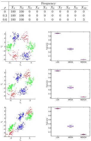
Our first simulation study is two-group classification for which LDA and SLDA are specifically de-signed: Xp×1|(Y =k)∼MVNp(µk,Σ) for k= 0,1,p= 10 predictors, andY ∼Bernoulli(0.5). The means were set as µ0= (−1,1,0T8×1)T and µ1= (1,−1,0T8×1)T, and Σwas the equicorrela-tion matrix with parameterρ, for levels ofρ given by 0, 0.3, and 0.6. A test set of size 20,000 was fixed to evaluate the performance of the classification methods. Training sets of sizen= 200 are used in the simulation, and 10-fold cross validation was used to select the tuning parameters for KDA, SKDA, SLDA, SCAD-Logistic, and SCAD-SVM. Results for 100 simulated data sets are in Table 2.1 and Figure 2.2.
Table 2.1 gives predictor selection frequencies by SKDA, SLDA, SCAD logistic regression, and SCAD SVM over 100 repetitions. Note that, onlyX1 andX2 are important for this example according to Proposition 1 in Section 2.6.2. Table 2.1 shows that the new nonparametric method SKDA performs competitively in terms of variable selection, even though the data generation strongly favors LDA and SLDA.
Table 2.1 Predictor selection frequencies for SKDA and SLDA for the study in Section 2.4.3.1.
Frequency
ρ X1 X2 X3 X4 X5 X6 X7 X8 X9 X10
0 SKDA 100 100 10 14 6 15 11 9 9 6
SLDA 100 100 1 1 3 1 2 2 3 3
SCADlogist 100 100 13 11 10 10 7 12 12 11
SCADsvm 100 100 13 14 11 15 18 12 9 10
0.3 SKDA 100 100 7 15 16 10 10 7 8 10
SLDA 100 100 2 0 0 1 1 0 0 0
SCADlogist 100 100 10 12 7 5 6 10 11 14
SCADsvm 100 100 6 6 5 5 9 5 7 9
0.6 SKDA 100 100 16 12 9 8 6 14 13 10
SLDA 100 100 0 0 0 0 0 0 0 0
SCADlogist 100 100 0 0 1 0 2 1 0 3
SCADsvm 100 100 0 2 1 1 0 2 0 3
over the independent test set across 100 repetitions are in the right panels. The top, middle, and bottom rows correspond toρ= 0, 0.3 and 0.6, respectively. As the setting is ideal for LDA, and SLDA, and only marginally less so for SCAD-Logistic and SCAD-SVM, these methods perform very well with SLDA having a slight edge. KDA neither exploits the marginal normality of the data, nor does it do variable selection, and thus performs poorly. However, although SKDA does not exploit the marginal normality, its performance in terms of classification error and selection is competitive.
2.4.3.2 Two-Group Mixtures of Equicorrelated Normals
−2 0 2 −3 −2 −1 0 1 2 3 x2 x 1
LDA SLDA KDA SKDA SCADlogist SCADsvm 0.08 0.09 0.1 0.11 0.12 0.13 0.14 0.15 Test error
−2 0 2
−3 −2 −1 0 1 2 3 x2 x 1
LDA SLDA KDA SKDA SCADlogist SCADsvm 0.05 0.06 0.07 0.08 0.09 0.1 0.11 0.12 0.13 Test error
−2 0 2
−3 −2 −1 0 1 2 3 x2 x 1
LDA SLDA KDA SKDA SCADlogist SCADsvm 0.02 0.03 0.04 0.05 0.06 Test error
Figure 2.2 Plots of typical training samples and boxplots of test errors for data generated withρ= 0
(top), 0.3 (middle), and 0.6 (bottom), from Section 2.4.3.1.
X1 and X2 (according to Proposition 1 in Section 2.6.2). Training sets of size 200 and a test set of size 20,000 are used. We setp= 10 and consider three different ρ values 0, 0.3, and 0.6. Results over 100 repetitions are reported in Table 2.2 and Figure 2.3 in a similar way as the previous example.
Table 2.2 Predictor selection frequencies for SKDA and SLDA for the study in Section 2.4.3.2.
Frequency
ρ X1 X2 X3 X4 X5 X6 X7 X8 X9 X10
0 SKDA 100 100 9 9 8 6 14 10 7 8
SLDA 0 0 5 4 3 5 6 6 4 8
SCADlogist 0 0 8 10 9 7 12 11 8 11
SCADsvm 38 38 50 54 55 56 59 56 53 57
0.3 SKDA 100 100 3 1 3 5 8 6 4 5
SLDA 0 0 4 5 5 3 6 6 6 9
SCADlogist 4 0 4 11 10 5 8 11 12 9
SCADsvm 46 39 52 52 51 54 56 60 60 60
0.6 SKDA 100 100 6 0 4 0 1 2 3 4
SLDA 2 1 4 5 7 3 4 3 7 6
SCADlogist 4 6 6 7 9 6 10 4 13 7
SCADsvm 51 54 46 52 52 53 56 56 60 59
poor performance of these methods is not unexpected in light of the data generation model. Variables X1 and X2 from one simulated training data set are plotted in the left panels of Figure 2.3 for three values ofρ: 0 (top), 0.3 (middle), and 0.6 (bottom). There is no good way to linearly separate the two classes well. Test error results are consistent as shown in the right panels of Figure 2.3. SKDA performs well whereas LDA, SLDA, SCAD logistic regression, and SCAD SVM perform like random guessing.
High dimensional case: We repeated the study changing only p= 10 to p= 50. Boxplots of the test errors over 100 repetitions are shown in right panels of Figure 2.4 for different methods and three values of ρ: 0 (top), 0.3 (middle), and 0.6 (bottom). Out of 100 repetitions, the frequency of X1 and X2 and average frequency of X3, . . . , X50 being selected by SKDA and SLDA are reported in Table 2.3.
The true classifier in this example is nonlinear, and thus LDA, SLDA, SCAD logistic regression, and SCAD SVM are misspecified. SKDA is nonparametric and thus more flexible. hence it performs well at both variable selection and classification accuracy.
−5 0 5 −5
0 5
x2
x 1
LDA SLDA KDA SKDA SCADlogist SCADsvm
0 0.1 0.2 0.3 0.4 0.5
Test error
−4 −2 0 2 4
−4 −3 −2 −1 0 1 2 3 4
x2
x 1
LDA SLDA KDA SKDA SCADlogist SCADsvm
0.1 0.2 0.3 0.4 0.5
Test error
−2 0 2
−3 −2 −1 0 1 2 3
x2
x 1
LDA SLDA KDA SKDA SCADlogist SCADsvm
0.15 0.2 0.25 0.3 0.35 0.4 0.45 0.5
Test error
Figure 2.3 Plot of one training sample (left) and boxplots of test errors (right) for the study in
Sec-tion 2.4.3.2 withp= 10 and three values ofρ: 0 (top), 0.3 (middle), and 0.6 (bottom).
−5 0 5 −5 0 5 x2 x 1
LDA SLDA KDA SKDA SCADlogist SCADsvm
0 0.1 0.2 0.3 0.4 0.5 Test error
−4 −2 0 2 4
−4 −3 −2 −1 0 1 2 3 4 x2 x 1
LDA SLDA KDA SKDA SCADlogist SCADsvm
0.05 0.1 0.15 0.2 0.25 0.3 0.35 0.4 0.45 0.5 Test error
−2 0 2
−3 −2 −1 0 1 2 3 x2 x 1
LDA SLDA KDA SKDA SCADlogist SCADsvm
0.15 0.2 0.25 0.3 0.35 0.4 0.45 0.5 Test error
Figure 2.4 Plot of one training sample (left) and boxplots of test errors (right) for the study in
Sec-tion 2.4.3.2 withp= 50 and three values ofρ: 0 (top), 0.3 (middle), and 0.6 (bottom).
2.4.3.3 Three-group, Normal Linear Discriminant Model
This is a 3-class example with p = 10 and an AR(1) correlation Σ = (σij) with σij = ρ|i−j|. We partition predictors with p1 = 2 and p2=p−2. Data are generated in two steps: generate Y uniformly over {1,2,3}. Conditional on Y, predictors are generated as X | (Y = 1) ∼ N(0,Σ); X | (Y = 2) ∼ N((θT12Σ11,θT12Σ12)T,Σ) with θ12 = (2,2
√
3)T; X | (Y = 3) ∼ N((θT13Σ11,θT13Σ12)T,Σ) with θ13= (−12,2
√
Table 2.3 Frequency ofX1 andX2 and the average frequency ofX3, . . . , X50being selected by SKDA and SLDA.
ρ Method (Average) Frequency X1 X2 X3, . . . , X50
0 SKDA 100 100 2.5
SLDA 1 0 4.2
SCADlogist 0 0 4.8
SCADsvm 31 23 44.6
0.3 SKDA 100 100 1.5
SLDA 1 0 4.4
SCADlogist 1 1 4.6
SCADsvm 28 37 41.8
0.6 SKDA 100 100 6.0
SLDA 1 2 2.1
SCADlogist 2 0 2.2
SCADsvm 47 43 45.7
the Bayes classification rule depends only onX1 and X2.
Table 2.4 Predictor selection frequencies for MSKDA for the study in Section 2.4.3.3.
Frequency
ρ X1 X2 X3 X4 X5 X6 X7 X8 X9 X10
0 100 100 1 1 1 0 1 1 0 0
0.3 100 100 0 0 0 1 0 0 0 0
0.6 100 100 1 0 0 0 0 0 0 1
−5 0 5 −6
−4 −2 0 2 4 6
x2
x
1
LDA MKDA MSKDA
0.05 0.1 0.15
Test error
−5 0 5
−6 −4 −2 0 2 4 6
x2
x
1
LDA MKDA MSKDA
0.05 0.1 0.15
Test error
−5 0 5
−6 −4 −2 0 2 4 6
x2
x
1
LDA MKDA MSKDA 0.08
0.1 0.12 0.14 0.16 0.18
Test error
Figure 2.5 Plot of one training sample (left) and boxplots of test errors (right) for the study in
Sec-tion 2.4.3.3.
in Figure 2.5. MSKDA reduces the test error in comparison to MKDA as a result of its variable selection. Because MSKDA performs variable selection very well, its performance is similar to that of LDA even though it is nonparametric.
{1,2,3,4,5}, and replacing the noninformative continuous X7 with the ‘new’ noninformative discreteX7 ∼Poisson(4). The selection frequencies for variablesX1, . . . , X10over 100 simulated data sets were 100, 100, 0, 1, 0, 1, 0, 1, 0, 1, respectively (compare to the top row of Table 2.4). A training sample and boxplots of test errors for this discrete case are displayed in Figure 2.6 (compare to the top row of Figure 2.5). These results are promising although far from a thorough study of SKDA and MSKDA with discrete predictors. The latter will likely prove fruitful just as the study of discrete predictors in the framework of kernel regression without variable selection has been; see [58] and [47] and the reference therein.
−5 0 5
0 2 4 6 8 10 12
x2
x
1
LDA MKDA MSKDA 0.06
0.08 0.1 0.12 0.14 0.16 0.18
Test error
Figure 2.6 Plot of a training sample (left) and boxplots of test errors (right) for the discrete
predic-tor simulation study in Section 2.4.3.3.
2.4.3.4 Three-Group, Mixtures of Equicorrelated Normals
This is another 3-class example with p= 10 and an AR(1) correlation Σ = (σij) withσij =ρ|i−j|. We also partition predictors with p1 = 2 and p2 = p−2. Data are generated in two steps: generateY uniformly over{1,2,3}. Conditional onY =k, predictors are generated asX |(Y = k)∼0.5N((θT1kΣ11,θT1kΣ12)T,Σ) + 0.5N(−(θT1kΣ11,θT1kΣ12)T,Σ), a mixture of two multivariate Gaussian distributions, for k = 1,2,3. Here θ11 = (5,0T9)T, θ12 = (2.5,5
√
3/2,0T8)T, and θ13= (2.5,−5
√
Table 2.5 Predictor selection frequencies for MSKDA for the study in Section 2.4.3.4.
Frequency
ρ X1 X2 X3 X4 X5 X6 X7 X8 X9 X10
0 100 100 0 0 0 0 0 0 0 0
0.3 100 100 0 0 0 0 0 0 0 0
0.6 100 100 0 0 1 0 0 0 1 3
−5 0 5
−6 −4 −2 0 2 4 6 x2 x 1
LDA MKDA MSKDA
0 0.1 0.2 0.3 0.4 0.5 0.6 0.7 Test error
−5 0 5
−6 −4 −2 0 2 4 6 x2 x 1
LDA MKDA MSKDA
0 0.1 0.2 0.3 0.4 0.5 0.6 0.7 Test error
−5 0 5
−8 −6 −4 −2 0 2 4 6 8 x2 x 1
LDA MKDA MSKDA
0.1 0.2 0.3 0.4 0.5 0.6 0.7 Test error
Figure 2.7 Plot of one training sample (left) and boxplots of test errors (right) for the study in
Sec-tion 2.4.3.4.
generation model, LDA is badly misspecified. Consequently LDA performs close to random guessing as seen in by Figure 2.7. MSKDA improves upon MKDA in terms of classification error due to its variable selection ability.
2.4.4 Illustrations with Real Data
2.4.4.1 Wisconsin Breast Cancer Data
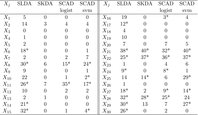
We apply SKDA to the Wisconsin Breast Cancer Data (WBCD) containing information on 569 patients, including a binary indicator of tumor malignancy (malignant/benign) and thirty purported predictors.1 We standardized each predictor to mean zero and variance one. In each repetition, we randomly select 300 observations as the training set and the remaining 269 are used as the test set to report performance by calculating the classification error for each method. Ten-fold cross validation was used for estimating tuning parameters. Test error results over 40 repetitions are reported in Table 2.6 and displayed in Figure 2.8. SKDA had a test error comparable to LDA, KDA, SCAD logistic regression, and SCAD SVM but a smaller test error than SLDA.
Table 2.6 Test error summary for 40 random splits of the WBCD data.
LDA SLDA KDA SKDA SCADlogit SCADsvm
Test Error Average 0.049 0.130 0.043 0.045 0.045 0.038 Test Error Std Dev 0.011 0.020 0.010 0.011 0.014 0.010
The average number of predictors selected by SKDA, SLDA, SCAD logistic regression, and SCAD SVM are 3.8, 11.0, 6.63, and 8.3, respectively. Predictor selection frequencies for SLDA and SKDA for this example are given in Table 2.7. SKDA selects far fewer predictors yet is competitive in terms of classification error.
LDA SLDA KDA SKDA SCADlogist SCADsvm 0.02
0.04 0.06 0.08 0.1 0.12 0.14 0.16 0.18
Test error
Figure 2.8 Boxplots of test errors for the WBCD example
Table 2.7 Predictor selection frequencies for SLDA and SKDA for the WBCD data example.
Aster-isks indicate variables selected using the entire data set.
Xj SLDA SKDA SCAD SCAD Xj SLDA SKDA SCAD SCAD
logist svm logist svm
X1 5 0 0 0 X16 19 0 3* 4
X2 14 3 4 4 X17 12* 0 0 0
X3 0 0 0 0 X18 4 0 0 0
X4 1 0 0 0 X19 10 0 0 0
X5 2 0 0 0 X20 7 0 7 5
X6 18* 0 0 1 X21 38* 40* 32* 40*
X7 2 0 2 7 X22 25* 37* 36* 37*
X8 30* 6 15* 24* X23 1 0 4 6
X9 9 0 0 1 X24 9* 0 8* 1
X10 22 0 1 2* X25 14 14* 6 29*
X11 26* 7 35* 17* X26 1 0 0 0
X12 10 0 2 2 X27 18* 2 9* 14*
X13 2 1 0 0 X28 32* 28* 25* 24
X14 21* 0 0 0 X29 30* 13 7 27*
X15 32* 0 1 4* X30 26* 0 2 0
2.4.4.2 Chemical Signatures
sites. We illustrate the application and performance of SKDA using data collected during the development of a remote measuring technology [73]. The data contain measurements of 38 chemical compounds recorded at each ofn= 170 sites. Secondary to the remote-sensing method development research, the data were clustered usingk-means clustering with k= 2 (and using all 38 compounds) ostensibly aligning with well type (dry, wet). We are not concerned with the accuracy or interpretation of this initial clustering. Rather for our illustration we take the classification as given and address the question of whether a smaller subset of the 38 compounds explains it. Because the study is still in progress, we identify the chemical compounds only as X1, . . . , X38.
The heat map in Figure 2.9 illustrates the data and classification. The figure is too small for the well labels, 1, . . . ,170, to be legible on the heat map plot. However, it is sufficient to know that the first 50 columns correspond to the “Y = 0” group, and that the last 120 columns correspond to the “Y = 1” group. Chemical compound labels, identified here only asX1, . . . , X38, are legible on the right vertical axis.
To assess the relative performance of methods on this data set we used 40 random splits of the data into training and test sets of sizes 136 and 34 respectively. The training data were analyzed using eight-fold cross validation to select tuning parameters where required. Average test errors (with standard errors) are reported in Table 2.8.
Table 2.8 Test error summary for 40 random splits of the chemical signature data.
LDA SLDA KDA SKDA SCADlogit SCADsvm
Test Error Average 0.15 0.38 0.17 0.02 0.31 0.02 Test Error Std Dev 0.06 0.07 0.06 0.03 0.03 0.03
1 2 3 4 5 6 7 8 910 11 12 13 14 15 16 17 18 19 20 21 22 23 24 25 26 27 28 29 30 31 32 33 34 35 36 37 38 39 40 41 42 43 44 45 46 47 48 49 50 51 52 53 54 55 56 57 58 59 60 61 62 63 64 65 66 67 68 69 70 71 72 73 74 75 76 77 78 79 80 81 82 83 84 85 86 87 88 89 90 91 92 93 94 95 96 97 98 99
100 101 102 103 104 105 106 107 108 109 110 111 112 113 114 115 116 117 118 119 120 121 122 123 124 125 126 127 128 129 130 131 132 133 134 135 136 137 138 139 140 141 142 143 144 145 146 147 148 149 150 151 152 153 154 155 156 157 158 159 160 161 162 163 164 165 166 167 168 169 170
x1 x2 x3 x4 x5 x6 x7 x8 x9 x10 x11 x12 x13 x14 x15 x16 x17 x18 x19 x20 x21 x22 x23 x24 x25 x26 x27 x28 x29 x30 x31 x32 x33 x34 x35 x36 x37 x38
0.1 0.3 0.5
Value Color Key
Figure 2.9 Chemical data heat map. First 50 columns (left to right) are the “Y = 0” group. Columns
within groups randomly ordered. Rows identify compoundsX1, . . . , X38.
regard to possible sparsity in a good classification rule.
2.4.5 Consistency of SKDA
We now establish consistency of SKDA. Below we establish the notation used for the statements of the results below, and in the proofs in the appendix Section 2.6.3.
Table 2.9 Predictor selection frequencies for SLDA and SKDA for the chemical signature data. Aster-isks indicate variables selected using the entire data set.
Xj SLDA SKDA SCAD SCAD Xj SLDA SKDA SCAD SCAD
logist svm logist svm
X1 26* 3 0 0 X20 11 0 0 0
X2 40* 40* 40* 40* X21 22* 0 0 0
X3 28* 0 0 0 X22 3 0 0 0
X4 29* 8 2 24* X23 10* 0 0 0
X5 23* 33* 15* 18 X24 23* 0 0 0
X6 13* 0 0 0 X25 11* 0 0 0
X7 19* 0 0 0 X26 9 0 0 0
X8 21* 0 0 0 X27 10 0 0 0
X9 25* 0 0 0 X28 19* 0 0 0
X10 20* 0 0 0 X29 23* 0 0 0
X11 21 0 0 1 X30 14* 0 0 0
X12 14* 0 0 0 X31 24* 0 0 0
X13 10 1 0 0 X32 20 0 0 1
X14 4 0 0 0 X33 17* 5 0 4
X15 16* 0 0 0 X34 22* 0 0 2
X16 10 0 0 0 X35 20* 3 1 10
X17 19* 2 0 1 X36 18* 0 0 0
X18 15 0 0 0 X37 14* 0 0 0
X19 10* 0 0 0 X38 16* 0 0 0
P(x)≡P(xI,xU) = π1f1(xI,xU)
π0f0(xI,xU)+π1f1(xI,xU). Note thatXU being unimportant means
P(xI,xU) =P(˜xI,xU˜ ) as long as ˜xI =xI. (2.13)
Note further that this partition is not unique since I ∪ {j} and U \ {j} is another partition of important and unimportant predictors for any j∈ U as long asI and U satisfy (2.13). To ensure uniqueness, assume thatI has minimal cardinality among all such partitions.
Extending the partition notation to ˜P(x)≡P˜(x;λ) =πb1f˜1(x)/(πb0f˜0(x)+bπ1f˜1(x)), we define
˜
P(xI,xU)≡P˜(xI,xU;λI,λU) =πb1f˜1(xI,xU)/(bπ0f˜0(xI,xU)+bπ1f˜1(xI,xU)), and`(λI,λU) = Pn
i=1
n
yilog( ˜P(xiI,xiU;λI,λU)) + (1−yi) log(1−P˜(xiI,xiU;λI,λU))
o
.
denotexA to be the subvector of xwith indices inA. We use this notation often. For example, sB andcB are subvectors ofs andcwith indices in B, and so on. By slight abuse of notation, letfk(xA) be the conditional density function of XA givenY =k fork= 0,1. For a symmetric kernelK(·), denoteµ2 =
R
t2K(t)dt and ν0 =
R
K2(t)dt.
Lemma 1 Consider an index subset A ⊂ {1,2, . . . , d}. Ifλj → ∞ asmink{nk} → ∞when j∈ Aandλj = 0otherwise, andmaxk
n Q
j∈Aλj/nk
o
→0, thenfbk(xA) =
1 nk
X
i:yi=k Y
j∈A
λjK(λj(xj−
xij)) is a consistent estimator of fk(xA) for k= 0,1. Asymptotically, the bias and variance
are given by Efbk(xA)−fk(xA) = µ2
2
P
j∈Af (2)
k;jj(xA)/(λ2j) +o(
P
j∈Aλ −2
j ) and Var(fbk(xA)) =
fk(xA)Qj∈A(ν0λj)/nk+o(n1kQj∈Aλj).
Lemma 1 shows that the estimator for the conditional density is consistent when all nonzero elements of λ diverge to infinity when n → ∞. We establish next that the estimator of the conditional density is not consistent when some elements ofλconverges to finite positive numbers while n→ ∞.
Lemma 2 Consider subsets A and B of {1,2, . . . , d}. If λj → ∞ as n → ∞ when j ∈ A,
λj → cj for some constant cj > 0 when j ∈ B, and λj = 0 otherwise, fbk(xA,xB) =
1 nk
X
i:yi=k Y
j∈A∪B
λjK(λj(xj −xij)) is not a consistent estimator of fk(xA,xB) for k = 0,1.
Asymptotically, we have Efbk(xA,xB) = R
sB( Q
j∈BK(sj))fk(xA,xB+D{cB}sB)dsB+
µ2 2
P
j∈Aλ12
j R
sB( Q
j∈BK(sj))fk,jj(2)(xA,xB+D{cB}sB)dsB+o(1 + P
j∈Aλ −2
j )and Var(fk(xA)) =
Q
j∈B(λj)
R
sB( Q
j∈BK(sj))fk(xA,xB+D{cB}sB)dsB
Q
j∈A(ν0λj)/nk+o(1 +n1kQj∈Aλj). The extra 1 in the little-o terms is due to the assumption thatλj →cj >0 for j∈ B.
Theorem 1 Assume that the domain X is compact andτ → ∞ and τd/n→ 0 as n→ ∞in (2.11). Then the optimizerλb = (λb1,λb2, . . . ,λbd)T is such that λbj → ∞ for j∈ I andbλj →0 for
j∈ U.
Corollary 1 Assume that the domain X is compact andτ → ∞ and τd/n→0 as n→ ∞ in
(2.12). Then the optimizer λb = (λb1,λb2, . . . ,λbd)T satisfies that bλj → ∞ for j ∈ I and bλj →0
for j∈ U.
2.5
Summary
We introduced a new approach to variable selection that adapts naturally to nonparametric models. The method is derived from a measurement error model likelihood, and exploits the fact that a variable containing a lot of measurement error is not useful for modeling. When the approach is applied to linear regression, the resulting new method is closely related to the LASSO, yielding a novel interpretation for the LASSO and lending credibility to the new MEM selection likelihood approach. When the approach is used for variable selection in nonparametric classification, a new method is obtained, sparse kernel discrimination analysis(SKDA). SKDA was shown to be competitive with existing methods in the case that the true classifier is linear (the case for which the existing methods were derived), and generally superior in cases where
the true classifier in nonlinear.
In Section 2.3.2 we showed that for linear regression with λj parameterized in terms of precisions, MESSO optimization is convex and amenable to efficient computation algorithms. For other cases that of interest MESSO optimization is not convex. For the simulation results and examples in this paper we used the MATLAB constrained minimization functionfmincon.2 We have also had good results with coordinate descent (modified to handle the sum-to-τ constraint) and a standard BFGS iteration after reparametrization to eliminate constraints, e.g., setting λj =τ η2j/(η12+· · ·+ηp2). A web search of“parallel coordinate descent”returns numerous recent technical reports describing promising modifications of coordinate descent that take advantage of parallel processing. We are investigating the use of these algorithms to enable MESSO to be routinely used with even larger-dimension problems than those studied in Section 2.4.3.2 (p= 50, 100).
to this dilemma in the MEM literature isregression calibration [11]. It provides a ready-made (approximate) solution to the construction of the MEM likelihoods (Step 2 of the algorithm in Section 2.2.3). Our initial attempts at using regression calibration to implement our MEM-based variable selection in generalized linear models are promising. Additionally, unlike in 1986, it is now feasible to compute likelihoods even when explicit forms are not available. Thus we anticipate that a second route to realizing the full potential of the MEM-based approach to variable selection will likely entail numerical (Monte Carlo) evaluation of MEM likelihoods.
Acknowledgments. The authors thank the entire review team and especially the Associate Editor and Editor for suggestions and comments that lead to substantial improvements in the paper. K. White was funded by NIH training grant T32HL079896 and NSF grant DMS-1055210; Y. Wu by NSF grant DMS-1055210 and NIH/NCI grant R01-CA149569; and L. Stefanski by NIH grants R01CA085848 and P01CA142538, and NSF grant DMS-0906421.
2.6
Appendix (Supplemental Files)
This section contains details provided in the supplemental files of [68]. Sections 2.6.2 and 2.6.3 are copied verbatim from the supplemental files. Section 2.6.1 contains additional details that are not in the supplemental files, but that facilitate presentation and understanding of the key convexity proof.
2.6.1 Equivalence of LASSO and LbSEL1-MESSO
We now prove the solution-path equivalence between maximizing LbSEL1 in (2.6) and LASSO.
We consider the transformation bσ2(λ) =
b
LSEL1−2/n, so that
b
σ2(λ) =VbY −Vb
T
XY
b
VX+D−1{λ} −1
b
VXY. (2.14)
MaximizingLbSEL1 is equivalent to minimizing bσ2(λ).