ABSTRACT
MOHAMED SAYEED. A parallel optimization framework for inverse problems. (under the direction of Dr. G. Mahinthakumar)
AN EFFICIENT PARALLEL OPTIMIZATION FRAMEWORK FOR INVERSE
PROBLEMS
by
MOHAMED SAYEED
A dissertation submitted to the Graduate Faculty of North Carolina State University
in partial fulfillment of the requirements for the Degree of
Doctor of Philosophy
DEPARTMENT OF CIVIL, CONSTRUCTION AND ENVIRONMENTAL ENGINEERING
Raleigh 2003
APPROVED BY:
_________________________ _________________________
(Dr. Ranji S. Ranjithan) (Dr. Abhinav Gupta)
BIOGRAPHY
ACKNOWLEDGEMENTS
I would like to thank all my committee members, teachers, colleagues and friends for all their help and understanding.
I would like to thank my advisor and co-chair Dr. G. Mahinthakumar for his valuable advice and support. He is the force behind this research and was always available for discussion.
I would like to thank Dr. John W. Baugh for being my co-chair and being supportive. I thank Dr. Ranji S. Ranjithan for being on my committee and for the valuable discussions we had on the optimization approaches. I appreciate Dr. Abinav Gupta for being my committee member.
I thank Emily Zechman for her help on MGA approach and Baha Mirghani for creating an animation of the GA performance.
I thank Dongju Choi and Leesa Breiger from SDSC, for doing the multi-cluster runs on the TeraGrid.
I wish to acknowledge North Carolina Supercomputing Center, Oak Ridge National Laboratory, National Center for Supercomputing Applications, San Diego Supercomputer Center and National Energy Research Supercomputing Center for providing the supercomputer resources necessary for this work.
I acknowledge the support indirectly provided by the PERC (Performance Evaluation Research Center) project (Dept. of Energy’s Scientific Discovery through Advanced Computing Program) subcontracted through ORNL from September 2001.
TABLE OF CONTENTS
LIST OF TABLES ...VI
LIST OF FIGURES ... VII
CHAPTER 1 – INTRODUCTION ... 1
1.1 INVERSE PROBLEMS... 2
1.2 COMPUTATIONAL METHODS FOR SOLVING INVERSE PROBLEMS... 3
1.3 ROLE OF HIGH PERFORMANCE COMPUTING... 6
CHAPTER 2 – RELATED RESEARCH IN GROUNDWATER INVERSE MODELING ... 9
2.1 NON-HEURISTIC APPROACHES... 9
2.2 HEURISTIC APPROACHES... 12
2.3 HYBRID OPTIMIZATION APPROACHES... 16
CHAPTER 3 – OPTIMIZATION METHODOLOGIES... 18
3.1 OVERVIEW OF GENETIC ALGORITHMS... 18
3.1.1 Genetic Algorithms for inverse modeling... 22
3.1.2 Binary/Integer GA Implementation... 23
3.1.3 Real Genetic Algorithm (RGA) Implementation ... 24
3.2 LOCAL SEARCH METHODS... 25
3.2.1 Nelder-Meade Simplex method (NMS)... 25
3.2.2 Hooke - Jeeves pattern search method (HKJ)... 27
3.2.3 Powell’s Method of conjugate directions (PWL) ... 28
3.2.3 Fletcher - Reeves conjugate gradient method (CG)... 29
CHAPTER 4 - PARALLEL IMPLEMENTATION ... 30
4.1 COUPLED FEM-GA-LS IMPLEMENTATION... 31
4.1.1 Hybrid GA-LS-FEM implementation ... 34
4.2 GRID IMPLEMENTATION... 35
CHAPTER 5 - TESTING AND EVALUATION ... 39
5.1 DESCRIPTION OF THE FEM TRANSPORT SIMULATOR... 39
5.2 BIOLOGICAL ACTIVITY ZONE IDENTIFICATION PROBLEMS... 40
5.2.1 Description of test problems ... 41
5.2.2 GA Encoding scheme ... 42
5.2.3 GA performance results ... 43
5.2.4 Integer encoding problem ... 46
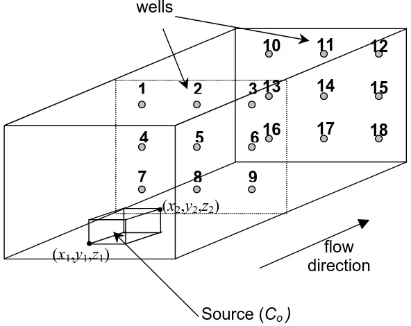
5.3 SOURCE IDENTIFICATION PROBLEMS... 47
5.3.1 Description of test problems ... 49
5.3.2 Hybrid GA-LS performance results ... 50
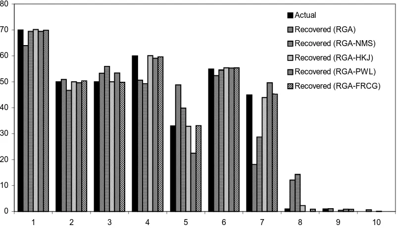
5.4 SOURCE RELEASE HISTORY RECONSTRUCTION PROBLEMS... 53
CHAPTER 6 - PARALLEL ARCHITECTURE AND PERFORMANCE ... 62
6.1 IBM SP3... 63
6.2 TERAGRID ITANIUM2 CLUSTERS... 64
6.3 PARALLEL PERFORMANCE... 65
6.3.1 Speedup ... 65
6.3.2 Load balance ... 67
6.3.3 Scalability analysis of hybrid approach... 68
6.4 GRID COMPUTING... 70
6.4.1 Results ... 71
CHAPTER 7 – RESEARCH CONTRIBUTIONS AND TOPICS FOR FURTHER RESEARCH... 75
7.1 RESEARCH FINDINGS... 75
7.2 RESEARCH ACCOMPLISHMENTS... 75
7.3 TOPICS FOR FURTHER RESEARCH... 76
BIBLIOGRAPHY ... 78
APPENDIX - A ... 85
PRELIMINARY INVESTIGATION OF NOISY-GA... 85
A.1 CURRENT APPROACH... 85
A.2 EXPERIMENTS... 86
A.3 RESULTS... 86
A.4 CONCLUSIONS... 87
APPENDIX - B ... 93
PRELIMINARY INVESTIGATION OF MODELING TO GENERATE ALTERNATIVES (MGA)... 93
B.1 MGA APPROACH... 93
B.2 TEST PROBLEM... 97
LIST OF TABLES
Table 5.1 Error in solutions obtained using various methods for the 3D source identification problem with ±10% noise in observation data. ... 53
Table 6.1 MPI Bandwidth for single and cross site run ... 72
Table 6.2 Runtimes for single and cross-site RGA-FEM simulations (using VMI1) 74
Table A.1 Results obtained for the single source release history reconstruction problem using noisy-RGA approach with multiple realizations and
heterogeneous hydraulic conductivity field. ... 89
LIST OF FIGURES
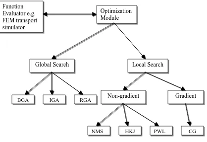
Figure 3.1 Different optimization algorithms available in the module for solving inverse problems... 19
Figure 3.2 Flowchart of genetic algorithms (GA)... 21
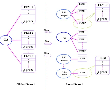
Figure 4.1 Schematic layout of parallel hybrid GA-LS-FEM optimization framework. The GA solution or the MGA alternatives are passed as initial starting guess to local search methods. The GA has P tasks (individuals)
evaluating using p processors for each function evaluation. The local search can be performed with n different/same methods using same or different initial starting points. ... 37
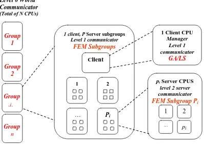
Figure 4.2 Three levels of MPI communicator hierarchy with multiple groups (n) performing GA/LS operations, and each group using different number of processors in a group (Pi.pi + 1). Pi is the number of server subgroups for group
i using pi processors for each FEM forward function evaluation. One processor
in each group is dedicated for GA or LS operations... 38
Figure 5.1 Problem setup for the biological activity zone identification problem. ... 41
Figure 5.2 Two types of zone encoding... 42
Figure 5.3 GA convergence history for 3-zone problem using uniform crossover. .. 44
Figure 5.4 GA convergence history for 3-zone problem using simple crossover ... 44
Figure 5.5 GA convergence history for 10-zone problem using uniform crossover. 45
Figure 5.6 GA convergence history for 10-zone problem using simple crossover. ... 46
Figure 5.7 GA convergence history for integer encoding problem. Encoding type B and simple crossover are used... 46
Figure 5.8 3D domain with a single source and observation well locations... 48
Figure 5.9 Concentration extrapolation scheme for a 2D problem. A similar
approach is applied to 3D cases. ... 48
method refer to every reduction in RSE value with forward function
evaluation. ... 51
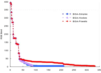
Figure 5.12 Convergence history of Hybrid BGA-LS approach for 3D source identification problem with ±10% noise in observation data. Iterations for Hooke’s and Powell’s method refer to every reduction in RSE value with
forward function evaluation... 52
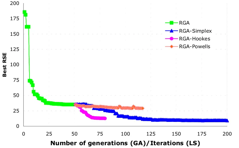
Figure 5.13 Convergence history of Hybrid RGA-LS approach for 3D source identification problem with ±10% noise in observation data. Iterations for Hooke’s and Powell’s method refer to every reduction in RSE value with
forward function evaluation... 52
Figure 5.14 Show’s the 2D source release history problem... 54
Figure 5.15 (a) Performance of the hybrid approach for a single source release history reconstruction problem without noise... 57
Figure 5.15 (b) Performance of the hybrid approach for a single source release history reconstruction problem with 10% random white noise in observation data. ... 57
Figure 5.16 (a) Performance of the hybrid approach for three sources release
history reconstruction problem without noise in observation data... 58
Figure 5.16 (b) Performance of the hybrid approach for three sources release
history reconstruction problem with 10% white noise in observation data. ... 58
Figure 5.17 (a) Performance of the hybrid (RGA-HKJ) approach for five-source release history reconstruction problem. Each curve represents a source... 59
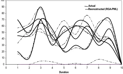
Figure 5.17 (b) Performance of the hybrid (RGA-PWL) approach for five sources release history reconstruction problem. Each curve represents a source... 59
Figure 5.17 (c) Performance of the hybrid (RGA-C.G) approach for five sources release history reconstruction problem. Each curve represents a source... 60
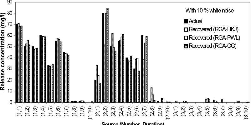
Figure 5.18 (a) Performance of the hybrid (RGA-HKJ) approach for five sources release history reconstruction problem with 10% random white noise added to the observation data. Each curve represents a source... 60
Figure 5.18 (b) Performance of the hybrid (RGA-PWL) approach for five sources release history reconstruction problem with 10% random white noise added to the observation data. Each curve represents a source... 61
Figure 6.1 Block diagram showing functional units of a power3-II architecture. .... 64
Figure 6.2 Standalone fine grained FEM simulation performance. ... 66
Figure 6.3 Total time taken by 129 processors to complete 10 generations using 1, 2, 4, and 8 processors per individual on the IBM SP. Population size is 128. ... 66
Figure 6.4 Time taken for 10 GA generations on the IBM SP using 2 processor per FEM simulation ... 67
Figure 6.5 Load balancing efficiency of self-scheduling algorithm. Processor speed is artificially simulated by varying number of time steps. ... 68
Figure 6.6 The scalability of hybrid approach using different processor count for local search, namely simplex. ... 69
Figure 6.7 Performance of single vs. cross-site fine grained parallelism ... 73
Figure A.1 Variation in RSE values shown for the different noisy-GA realization solutions using the full hydraulic conductivity sample set (100)... 89
Figure B.1 Distribution of MGA solutions for 50 runs. Solutions marked with circles are the MGA solutions. ... 99
Figures B.2 (a) and (b) Difference between MGA alternatives 1 and 2 for selection based on fitness for two different runs. ... 100
CHAPTER 1 – INTRODUCTION
Inverse problems that are governed by large-scale partial differential equations (PDE) require significant computational resources and can be several orders of magnitude more computationally challenging than the corresponding forward problem (i.e., prediction) because repeated solutions of the forward problem are necessary. These problems are particularly challenging in subsurface contaminant characterization because the forward model can consist of several coupled large-scale nonlinear partial differential equation systems that can vary in three-dimensional space and time. Recent advances in search techniques such as genetic algorithms (GAs) and emergence of advanced computing resources such as the computational grid (networked supercomputers), have opened up new possibilities for solving these inverse problems. The most common approach for solving subsurface characterization inverse problems is the use of gradient-based optimization methods. While these methods are very powerful and are appropriate in many situations, they lack the generality of non-gradient approaches (e.g. genetic algorithms, simulated annealing) and are less suited for emerging parallel computing environments.
GAs are popular global search procedures for discrete as well as continuous problem domains, but yet under-explored for solving these problems. The GA search process is enhanced by the use of local search (hybrid approach). The main themes for the proposed research are to investigate: (i) hybrid optimization approaches (global and local searches) and, (ii) parallel computing techniques to solve inverse problems (in the groundwater area).
chapter presents the results of testing and validating the hybrid optimization methodology. Information on parallel architecture, parallel performance results and grid-computing results are discussed in 6th chapter. The 7th and final chapter summarizes research contributions and topics for further research work. In Appendix – A, the noisy-GA approach is investigated for problems with parameter uncertainty. In Appendix B, a preliminary investigation of the modeling to generate alternatives (MGA) approach is carried out for addressing the non-uniqueness problem.
1.1 Inverse Problems
An inverse problem involves the estimation of certain quantities based on indirect measurements of other dependent quantities. This research focuses on groundwater inverse problems. Inverse problems also arise in other diverse fields such as geophysical exploration, medical imaging, non-destructive evaluation, inverse heat conduction or diffusion problems, and signal processing. In signal and image processing one tries to recover the original (uncorrupted) signal from the filtered signal with noise. Use of computer aided tomography and magnetic resonance imaging in medical diagnosis, has lead to the development of algorithms for the inversion of the Radon transform. The exploration of oil is often facilitated by knowledge of the electrical conductivity structure of a rock formation. The conductivity itself is ascertained from establishing a magnetic field in the rock formation by measuring the induced currents. Seismic exploration yields measurements of vibrations recorded on the surface. These measurements are only indirectly related to the subsurface geological formations that are to be determined.
Other inversion examples are: loading a concrete specimen and measuring its deformation to determine material properties such as Young’s modulus and Poisson ratio, or the deflection of the bridge is measured to access the condition of cables and deck [Bui 1993]. A performance based dynamic structural design approach using inverse problem formulation has been developed [Takewaki 2000].
A number of groundwater problems such as estimating hydraulic conductivity distributions, biological activity zones (BAZ), dense non-aqueous phase liquids (DNAPL), or contaminant sources location and release history have been solved using the inverse problem formulation. A very good reference for inverse problems in ground water modeling is by Sun, 1994.
While common enough in practice, groundwater problems such as these are notoriously difficult to solve because of several factors namely, insufficient observation data, error in model or input data, etc. During the past several year’s significant developments in probability and control theory methods have helped solve such complex inverse problems [Sun 1994]. Most of the inverse problems are characterized by an unusually high sensitivity to perturbations (deterministic as well as stochastic) in the data so that a small change in the measurements results in disproportionate error in the recovered signal. Techniques such as regularization methods have been developed to deal with this Ill-Posedness. Thus, solving such inverse problems is not only numerically challenging, but they also demand large computational resources.
1.2 Computational methods for solving inverse problems
As stated earlier, before solving an inverse problem a mathematical model for solving the forward problem should exist. So a concise discussion on mathematical modeling of forward problems is provided next. Mathematical models can be broadly classified in to four types: (i) Deterministic models and stochastic models depending on whether random variables appear in the model; (ii) Linear models and nonlinear models depending on whether the equations are linear or nonlinear; (iii) Stationary and dynamic models, depending on if the time variable is included and, (iv) Lumped parameter models and distributed parameter models depending on whether the space variables are included. In groundwater modeling distributed parameter modeling is preferred because it is more general, more accurate and more suitable for the planning and management of groundwater resources. A distributed parameter model is often described by a PDE or a set of PDEs and may be classified in to one or several of the above types. Generally, the distributed parameter model involves the following components: it may have both spatial and temporal properties, system parameters that characterize the geometry and/or physical nature of the system, initial condition of the system described by one or more subsidiary conditions, control variables representing excitation of the system such as pumping, artificial recharge etc., and state variables that describe the state of the system, such as head, concentration etc. Solving a forward problem implies to determine state parameters when the time-space region, system parameters, subsidiary conditions and control variables are known. The solution can be obtained analytically or using a numerical approach. Analytical solutions are however available only for simple problems. The solutions can be obtained by superposition of fundamental solutions, separation of variables, Laplace transformation, Fourier transformation and other integral transformations. Numerical methods use discretization of the time-space domain in to elements and nodes. The governing system of equations (PDEs) is then discretized and replaced at these nodes by a system of algebraic equations. The solution of the equations can be obtained using different methods such as finite difference methods, finite element methods, boundary element methods and their variants and hybrids, including the hybrids
If a mathematical model is available to solve a forward problem then it can be used in an iterative fashion to solve the inverse problem. However the accuracy of the forward model is no guarantee for the quality of the solution obtained in the inverse approach. This is normally referred to as the Ill-Posedness of the inverse problem. Three main criteria describe the Ill-Posedness of the inverse problem
Non-existence: The solution may not exist for the observation data.
Non-uniqueness: The solution may not be unique because different conditions may give same observation data.
Instability: A small change in input results in a disproportionate output.
The above three properties are associated with many of the inverse problems encountered in real applications.
As stated earlier inverse problems can be solved in both deterministic and stochastic frameworks by direct or indirect methods. Indirect methods require repeated solutions of the forward problem. Many of the methods solve the problem by using an output least squares criterion, which is a measure of the error between the measured and the computed values. In general, direct methods can only be used for solving inverse problems governed by linear system of equations. The commonly used direct methods are the matrix method and the linear programming method. The matrix method reformulates the linear least squares problem as a set of matrix equations and solves it directly. The matrix method normally yields highly ill conditioned matrices and is very sensitive to measurement errors. Linear programming methods can be used to solve inverse problems governed by linear equations. Direct methods have very limited applicability to groundwater inverse problem due to the distributed nature of the parameter space, non-linearity in the governing equations and measurement errors.
Levenberg-Marquadt, Gauss-Newton, conjugate gradients and sequential quadratic programming methods. The gradient-based approaches use the gradients to find the solution and hence require the decision space to be continuous (smooth). Thus, the gradient methods are not suitable for discrete optimization problems. However, the gradient methods tend to converge faster than non-gradient based approaches if: (i) the objective function is continuous and differentiable, (ii) the search space is fairly smooth and not convoluted and (iii) the quadratic assumption is valid near the optimum (for some approaches).
Non-gradient methods start with one or more initial guesses and follow a set of rules to move towards the solution. These optimization methods can be global or local. Examples of global approaches are genetic algorithms (GAs) [Holland 1975, Goldberg 1989], simulated annealing, particle swarm optimization (PSO) [Kennedy and Ehart 1995], and the DIRECT method [Floudas and Pardalos 2001]. Examples of local non-gradient approaches are, Nelder-Meade simplex method, Hooke-Jeeves pattern search method, and Powell’s method of conjugate directions. Non-gradient based techniques such as GAs offer great flexibility in problem formulation and can handle discontinuities in the search space. Furthermore, they can generally explore a larger search space than gradient-based approaches. As stated earlier GAs are generally preferred for discrete or discontinuous domains and is the global method of choice for this research. GAs can also be used effectively (real GAs) for problems that are not inherently discrete. The focus of this research is to establish a parallel optimization framework for solving groundwater inverse problems.
1.3 Role of high performance computing
and offered challenges for the development of new and efficient mathematical models. High performance computing (HPC) offers the ability to compute solutions to problems not possible on desktop machines. It provides the ability to: (i) use larger and more detailed computational grids, (ii) develop more complete computational models of physical processes, and (iii) perform large number of simulations under different conditions. HPC is enabled by large parallel computers, powerful vector processors, or a network of individual workstations. These parallel computers link processors or individual workstations together to increase computational power and use high-speed, large-memory-capacity computers. Algorithmic improvements with state-of-the-art numerical techniques such as adaptive meshing, multigrid, and particle methods are needed in the next generation of high-performance simulation codes (e.g., groundwater).
For problems that require significant computational resources, parallel computing on supercomputers or newly emerging “grid computing” on a network of geographically distributed heterogeneous supercomputers connected by high-speed network can be used. Also, distributed computing on cluster of networked workstations can be helpful. Parallel computing requires knowledge of parallel machine architectures for efficient implementation of parallel applications and efficient parallel numerical algorithms. One or more parallel programming tools such as MPI [Message Passing Interface, Gropp et al. 1999; Dongarra et al. 1994], OPENMP [www.openmp.org], PVM [Parallel Virtual Machine; Giest et al 1994], etc., are available on high performance computers for use. Currently MPI has emerged as the de-facto standard and is available on almost all supercomputers. Parallel codes using MPI are portable. MPI implementations supporting many languages including popular HPC languages such as Fortran and C are available.
Parallel programming is notoriously difficult because it lacks the single thread of control that one would have in a conventional serial program. In addition, the data used in parallel computation are probably spread across a number of distributed computer systems. This is done to capitalize on locality by leveraging faster local data accesses against more costly remote data accesses. Often, the data “decompositions” that make a parallel program the fastest are the ones that are the most complicated [Kohl 1997].
CHAPTER 2 – RELATED RESEARCH IN GROUNDWATER
INVERSE MODELING
Much of the previous work in groundwater inverse modeling has been in model calibration aimed at fitting a few parameters (determine a few parameters in the forward model based on observation data). With the development of sophisticated forward models in recent years inverse modeling can now be used for obtaining detailed information about the subsurface. This subsurface information is critical to the efficacy and cost efficient groundwater management strategies. The following sections provide an overview of previous research using optimization approaches for groundwater modeling.
2.1 Non-heuristic approaches
A large amount of research has been done in using gradient-based approaches for solving groundwater inverse problems (e.g. Gorelick et al 1983, Wagner 1992, Sciortino et al. 2000, Mahar and Datta 2000). Gorelick et al (1983) used least squares regression and linear programming for solving a hypothetical two-source groundwater contaminant problem. They assumed a linear model and incorporated the solute transport model as constraints in a response matrix approach [Gorelick 1982; Gorelick and Remson 1982b] for solving. Two hypothetical scenarios were studied: (1) locating unknown pollutant sources under steady state from concentration data collected at a few well locations, and (2) reconstructing the release history and location of a source using a complex two dimensional (2-D) transient system with several monitoring wells. For the steady state case there were more unknowns than the number of constraining equations. A mixed integer programming method with additional restrictions was used. The results obtained were spurious and detracted from true values. For the transient case both methods identified the pollution source and the disposal episodes, but contained some errors in determining the disposal flux magnitudes. The method is restricted to cases where data are available in the form of break through curves.
minimum relative entropy approach - MRE [Woodbury and Ulrych 1996, Skaggs and Kabala 1998, Woodbury et al. 1998], Tikhonov regularization - TR [Skaggs and Kabala 1994, Liu and Ball 1999], constrained nonlinear optimization [Mahar and Datta 2000, 2001], and Levenberg-Marquadt minimization [Sciortino et al. 2000] have been used. A paper by Atmadja and Bagzoglou (2001), gives a state of the art report on mathematical methods for groundwater pollution source identification.
The regularization methods such as TR and MRE try to alleviate the problem of ill-posedness and computational complexity of inverse problems. For example, the TR method removes discontinuity in the solution space by smoothing the objective function (either directly or indirectly). This addresses the problem of instability (small changes in decision variables lead to large variations in objective function) and non-uniqueness (multiple solutions) by forcing the convergence to the ‘simplest’ solution (solution that has the smoothest structure). There is no guarantee, however, that this is the best solution. MRE method treats each element of the release history as a random variable. The MRE inversion is a method of statistical inference. It constructs a probability density function (pdf) for the random variables representing the solution based on prior information and measurement data; the solution is the mean of this pdf. Neupaur et al. (2000) made a comparative study of TR and MRE methods for different source release history recovery problems. The results show the quality of solutions obtained by these methods to be input and problem dependent.
convex even in the absence of observation errors. Also, the results produced by the model varied according to the number and location of the observations.
Datta et al. (1989) developed an expert system using statistical pattern recognition techniques to identify sources of groundwater pollution for hypothetical example problems. The model developed by Gorelick et al. (1983) was used as a preliminary screening model within the expert system. Performance of their method was found encouraging in general for the example problems and specifically good under conditions of missing observed-concentration data. Bagtzoglou (1992) presented the application of a random walk based model for identification of pollutant sources in groundwater. Wagner (1992) combined nonlinear maximum likelihood estimation with ground-water flow and solute transport simulation to simultaneously estimate the aquifer parameters and a distributed pollutant source term.
real-life scenarios when initially the potential source locations are unknown and where measurements and parameter estimates are erroneous and/or uncertain. However their study did not address the effect of parameter uncertainty and only a limited numbers of cases were tested.
Following their work in 1996, Mahar and Datta (1997, 2000 and 2001) solved different types of source identification problems using non-linear programming approach. They used finite differences and the finite difference equations as constraints to model two-dimensional forward flow with steady state or transient and transport problems. The governing equations for the physical processes were embedded in the optimization model. They solved the resulting nonlinear programming problem by a quasi-Newton constrained optimization method. The model is tested for 2 or 3 potential source locations, both with and without perturbed observation data and also with data gaps. The model was not very robust because of the nonconvex and nonunique nature of the inverse problem and because the results were dependent on the initial guess provided to the method. They extended the model to simultaneously estimate the aquifer parameters (2001).
2.2 Heuristic approaches
While heuristic techniques such as GAs have been used widely for groundwater management problems [McKinny and Lin 1994; Wang and Zheng 1998], or for optimal placement of monitoring wells [Cieniawski et al. 1995, Ritzel et al. 1994, Huang and Mayer 1997, Katsifarakis et al. 1999] they have not been used as extensively for solving groundwater inverse problems.
with data gaps, for both without noise and random noise in the synthetically generated reference data cases. Based on their study they concluded that their IGA provides an efficient and robust means for solving any quadratic optimization problems with linear equality constraints.
Katsifarakis et al. (1999) used boundary element method (BEM) approach for modeling groundwater flow and transport and coupled it with GA to solve common groundwater management and inverse problems. The application examples studied are (1) determination of transmissivities in zoned aquifers, both with and without field measurement errors, (2) minimization of pumping cost from a group of wells, and (3) hydrodynamic control of a contaminant plume. They claimed that the method performed satisfactorily.
Mahinthakumar et al. (1999) used GAs for identifying zones of biological activity in the subsurface. They used a parallel computing environment for solving, as repeated three-dimensional finite-element forward function evaluations are required for every individual in a GA population. The simulations performed showed the effective application of GAs in inverse groundwater modeling.
reasonably accurate results, noisy genetic algorithms perform best without extensive sampling [Miller and Goldberg, 1996]. On the basis of Aizawa and Wah’s (1994) sampling strategy for noisy GA’s, the following approach was used. For the first four generations sampling size was set to 5 and was increased by five sample sets every four generations. After twelve generations fittest four designs from the previous four generations (i.e., 9-12) were tested by simulating each with five hundred sample sets. If any of the four designs are successful in meeting the risk criteria for at least 90% of the realizations, then sample size was not increased and the optimization process continued for four more generations before termination. Otherwise, the sample size is increased by five sample sets in the same manner described above with a test for four fittest designs from the previous four generations every four generations until successful termination or until a maximum number of generations was reached. Based on a case study, the authors concluded that noisy GA was capable of generating highly reliable designs from relatively small number of sample sets and efficient for computationally intensive groundwater management models. The authors suggested the need for further investigation of sampling strategies and termination criteria that affect GA efficiency, the values of the decision variables for the optimal design, and the reliability of the optimal design.
Yoon and Shoemaker (2001) proposed an improved real-coded GA (RGA) for bioremediation. They proposed a new technique for crossover and selection (replacement) process of GA. The RGA developed was tested for two hypothetical aquifers developed by Minsker (1995). Based on the study they reported RGA was efficient and computationally accurate than binary encoded GAs used in previous groundwater research.
problems with explicit linearized constraints, which are then solved by GA. In the search stage GA is used to search for local optimal solution with in the subdomain and closer to the previous solution. The authors applied the methodology to test several groundwater applications for a single source in a heterogeneous unconfined aquifer system. They solved the release history reconstruction problem for known source location, unknown source location, and release history with some observation data missing (gap). Based on their study of the above problems they claimed PGA technique as robust and computationally efficient. Several observations about the factors that influence the solution of the source identification problem were also reported.
Giacobbo et al. (2001) solved the inverse problem of parameter estimation by GA for groundwater contaminant transport. They analyzed the sensitivity of the model to the unknown input parameters from the speed of convergence and stabilization of the GA. They showed that the GA evolves towards convergence by stabilizing first the most important parameters (parameters that influence the model output most) and later the parameters that influence the output less.
Shieh and Peralta (2003) used parallel recombinative simulated annealing (PRSA) for optimizing in-situ bioremediation system design. PRSA is a global optimization algorithm with convergence properties of simulated annealing (SA) and parallelism of GA. The proposed model uses BIOPLUME II model to simulate aquifer hydraulics and bioremediation, and PRSA to search for an optimal design. They solved for an optimal pumping (extraction/injection) strategy that minimizes total system cost, reduces contaminant concentration to the cleanup standard, and prevents contaminant plume migration. For the test problem the PRSA approach performed better than SA and GA. They claimed the approach to be efficient and flexible for optimizing system installation design and time-varying pumping.
2.3 Hybrid optimization approaches
Very limited amount of work has been done to date using hybrid optimization approaches for solving groundwater inverse problems [Heidari and Ranjithan 1998, Pan and Wu 1998]. Heidari and Ranjithan used a hybrid GA- truncated Newton search for a two-search approach for a two dimensional hydraulic conductivity estimation problem. Pan and Wu (1998) used a simulated annealing – simplex approach for estimating unsaturated flow parameters for a one-dimensional column experiment.
process. In general the hybrid approach performed better. Also, SAHGA is more robust than NAHGA because local search is applied only when it is necessary and the performance does not change for a broad range of different parameter values.
CHAPTER 3 – OPTIMIZATION METHODOLOGIES
This chapter describes the optimization methodologies used in this research. The research uses hybrid optimization approaches for solving inverse problems. The sections that follow discuss GA methodology (both binary/integer and real GA) and the four local search methods, Nelder-Meade simplex (NMS) method, Hookes and Jeeves pattern search (HKJ) method, Powells conjugate directions (PWL) method, and Fletcher and Reeves conjugate gradient (CG) method. Figure 3.1 shows the optimization algorithms implemented in this research.
3.1 Overview of Genetic Algorithms
Figure 3.1 Different optimization algorithms available in the module for solving inverse problems.
During the GA search process, the population is subjected to several probabilistic operators that are analogous to natural selection, mating (including genetic recombination), and mutation. In the selection step, pairs of solutions are selected for reproduction from the population, with fitter individuals being selected more frequently. Each pair of solutions may then undergo mating, or crossover, in which their vectors are recombined to form new solutions, which are placed into a new population. The selection and mating steps continue until the new population is the same size as the previous population, which is then discarded. After the new population has been generated, mutation is used to modify a small number of genes in the population. This step introduces new traits that may not have been present in the initial population. Mutation may also reintroduce good traits that may have been lost through the probabilistic selection operator. An additional operator called elitism is used in most GA applications. Elitism, which generally occurs after mutation, is used to guarantee that the best individual in a population is not lost.
Function Evaluator e.g. FEM transport simulator
Optimization Module
Global Search Local Search
BGA IGA RGA Non-gradient Gradient
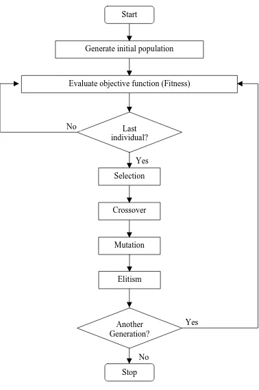
The flowchart for GA is shown in figure 3.2. The steps of evaluating the population, selection, mating, mutation, and elitism constitute one iteration, or generation. Because fitter solutions are more likely to be selected for mating, the incidence of good traits in the new population generally increases with each additional generation. Crossover serves to test these traits in many different combinations. GA schema theorem predicts the frequency of good traits (and good combinations of traits) to increase exponentially as new generations are formed. As this occurs, the GA converges to increasingly better solutions. Improvements in fitness, however, diminish as the population diversity decreases and the population converges towards a good solution. Stopping criteria such as “10 generations without improvement” and a minimum population diversity are often used to terminate the algorithm when improvements are sufficiently small and infrequent. These concepts are well described in many texts, including Goldberg (1989), Davis (1991), and Michalewicz (1996).
Figure 3.2 Flowchart of genetic algorithms (GA).
Start
Generate initial population
Evaluate objective function (Fitness)
Last individual?
Selection
Crossover
Mutation No
Yes
Another Generation?
Stop No
3.1.1 Genetic Algorithms for inverse modeling
As described earlier, GA starts with a set of potential solutions, or population and the performance of each solution is characterized by a fitness value. In the context of inverse problems, fitness is calculated using a forward solve and is inversely proportional to the difference between computed and observed values. One of the drawbacks of GA is that it is computationally intensive if the fitness evaluation (or objective function) is expensive. In this application, the objective function to be minimized is the root square error (RSE) between the observed and the computed output concentration signals at a few selected points in the domain. RSE is given by
2
1
( )
n
obs calc
i i
i
RSE C C
=
=
∑
−Where Ciobs is the observed concentration and calc i
3.1.2 Binary/Integer GA Implementation
The BGA and IGA implementations are required for the BAZ identification problem (see section 5.2). A slightly enhanced version of the Simple Genetic Algorithm (SGA) presented in Goldberg (1989) is used for the BGA and IGA implementations. The primary modifications are elitism (always retain the best solution in the new population), additional selection procedures (tournament selection in addition to the original roulette wheel selection), additional crossover strategies (uniform and multi-point crossovers in addition to the original simple crossover), and support for both binary and integer encoding. An adaptive mutation operator is implemented so that the mutation probability can be progressively reduced when the RSE of the best individual drops below an arbitrary threshold value (if the correct solution is known a priori then this threshold value can be set close to zero). A restart option is implemented so that the simulation can be restarted from the last completed generation.
In the simulations performed the following steps are involved:
(1) Encode the unknown zone locations as binary or integer strings.
(2) Generate an initial random ensemble of strings (with a user-defined bias) equal to the number of individuals in a population or population size.
(3) Perform transport simulation for each individual by decoding the strings into zone locations.
(4) Compute RSE for each individual by computing the difference between the observed (stored in a file) and computed output signals.
(5) Select the individuals that perform best (those giving a smaller RSE) using an appropriate selection strategy and mate the strings randomly (using an appropriate crossover strategy – single point, uniform, multiple point) to produce the next generation for individuals.
(6) Repeat steps 3 – 5 until convergence or up to prescribed maximal number of generations.
generations or the probability distribution of the entire population at the end of simulation can be chosen as the optimal solution.
3.1.3 Real Genetic Algorithm (RGA) Implementation
Real GA follows the same steps as BGA/IGA. As stated before, for RGA decision variables are represented as a vector of real variables (within some bounds). For source identification and release history reconstruction problems, RGA is more suitable as the decision variables (source location coordinates, concentrations, and time history of concentration release) are inherently real. The real encoding can represent large domains with a smaller string length when compared to its binary representation without sacrificing the precision of numbers. Also increasing the number of bits considerably slows down the algorithm [Michalewicz (1996)]. The concepts and operators (selection, crossover, mutation and replacement) are very similar to BGA.
The RGA implementation has four different crossover strategies simple, uniform, arithmetic and heuristic crossovers. In arithmetic crossover a linear combination is performed using the following expression, if x1 and x2 are crossed then the two offsprings
will be x1′= rx1 + (1-r)x2 and x2′ = rx2 + (1-r)x1, where ‘r’ is a random number generated
between 0 and 1. In heuristic crossover a single offspring is produced from two parents x1 and x2 according to this rule: x3 = r(x2-x1) + x2, where ‘r’ is another random number
generated between 0 and 1, and parent x2 is not worse than x1. The algorithm uses a
'
k k
x = −x dtand (dt= xku −xk)( (1r −a))b,
Where, x - upper bound for the element of the chromosome string, r- random ku number between 0 and 1, a is the ratio of generation number to maximum number of generations and b is a system parameter determining the degree of non-uniformity (assumed to be 1). For all the simulation experiments performed using real GA, non-uniform mutation is used. Additional information on real GAs is available in many books on GAs such as by Michalewicz (1996).
3.2 Local search methods
Non-gradient based unconstrained optimization methods are implemented for local searches. These methods were selected because they do not require the computation of gradients and are easier to program. The methods are: (1) Nelder-Meade Simplex, (2) Hooke and Jeeves pattern search, (3) Powells method of conjugate directions and (4) Fletcher-Reeves conjugate gradient method. The following subsections give brief description of these methods. More details are available in standard optimization texts such as Belegundu and Chadrupatla (1999).
3.2.1 Nelder-Meade Simplex method (NMS)
The initial simplex of n+1 corners is constructed from the initial guess by perturbing each point by a fixed amount. The points with highest, second highest and the least function values are selected. The point with largest function value is excluded and mean of the points is computed. A new point is obtained by reflecting about the mean and the forward function is evaluated at the reflected point. If the reflection is successful then the point is further expanded. If the expansion step fails then the point is contracted. If both expansion and contraction stages fail then the previously reflected point is accepted. If reflection, expansion and contraction stages fail, then a scaling operation is used to scale the point with the least function value, which shrinks the simplex. The operations described above can be represented in notation form. Let X , h X , and s X be l the points with highest, second highest and lowest function value points and X mean of b the points excluding highest, given as
1
1
1 n
b i
i i h
X X
n
+
= ≠
=
∑
. The new points during reflection,expansion, contraction and scaling stages are calculated as follows,
( )
r b b h
X =X +r X −X ←Reflection
( )
e b r b
X =X +e X −X ←Expansion
( )
c b b h
X =X +c X −X ←Contraction
( )
i l i l
X =X +s X −X ←Scaling
The coefficients r, e, c and s are assumed as 1, 1, 0.5 and 0.5 respectively. The steps are repeated until the convergence or stopping criteria is satisfied.
3.2.2 Hooke - Jeeves pattern search method (HKJ)
Hooke and Jeeves method is a simple yet powerful exploratory pattern search method that can be applied to discrete and continuous optimization problems. The method has two basic steps: (i) explore the neighborhood of the current point and establish a pattern to move, (ii) move to a new point using the established pattern. The exploratory step consists of sequentially perturbing (positively and negatively) the current solution vector (starting with an initial guess) in each direction by a fixed amount (step size) such that an improvement is found in the solution. If there is no improvement after perturbations in all directions are completed, then the exploration is conducted with a reduced step size. The step size is progressively reduced until an improvement is found or it reduces below a prescribed tolerance (say 1e-6) in which case the algorithm is terminated. When an improvement is found, a pattern direction vector is evaluated by taking the difference between the improved solution vector and the old solution vector. In the second step, the new solution is found by extrapolating the old solution along the pattern direction.
A step size is chosen and exploration is started from the given starting point. AssumeX is the initial starting point with n decision variables, where i0 e is the unit i vector (n * 1) along direction i and s is the step size. The exploration and pattern step can be calculated as follows,
0
0
, 0
Exploration
, for and , 1,..,
, and , 1,..,
Pattern search
2 1,..., and ( exploration succesful) ij i
ij i i
iJ iJ i
X X i j i j N
X X e s for i j i j N
X X X i N J j
= ≠ =
= ± = =
= − = =
3.2.3 Powell’s Method of conjugate directions (PWL)
Powell’s method of conjugate directions carries out minimization along successive directions that are conjugate with respect to all previous directions. Powell developed an idea of computing conjugate directions without using derivatives [Powell (1964)]. It requires N single variable minimizations per iteration and sets up a new conjugate direction at the end of each iteration. The procedure for computing the conjugate direction set is as follows [Press et al. 1996],
Initialize the set of directions U toi the basis vectors, Ui =ei for i=1,....,N Repeat the following sequence of steps until function value stops decreasing: Save starting position as P 0
For i=1,,N move Pi−1 to the minimum along direction U and call this point Pi i
Fori=1,,N set Ui+1 =Ui Set UN =PN −P0
Move PN to the minimum along direction UN and call this point P0
Reinitialize the set of directions Ui to the basis vector ei after N or N+1 iterations.
1
1 1 1
2 2 1 1 1
1
(1) Start with an arbitrary initial point .
(2) Set the first search direction ( ) . (3) Find the point according to the relation = Where is the optimal step length in
X
S f X f
X X X λS
λ = −∇ = −∇ + 1 2 1 2 1
the direction . Set 2 and go to the next step. (4) Find ( ), and set
(5) Compute the optimum step length in the direction , and find t
i i
i
i i i
i
i i
S i
f f X
f
S f S
f S λ − − = ∇ = ∇ ∇ = −∇ + ∇ 1 1 1
he new point
(6) Test for the optimality of the point . If is optimum , stop the process. Otherwise, set the value of 1 and go to step 4.
i i i i
i i
X X S
X X i i λ + + + = + = +
3.2.3 Fletcher - Reeves conjugate gradient method (CG)
Fletcher and Reeves conjugate gradient method is a steepest descent method and can be considered as a conjugate directions method involving the use of the gradient of the function. By evaluating the gradients of the objective function, new conjugate directions are set up at the end of each iteration and hence, faster convergence can be achieved. The iterative procedure for the method is given below [Rao 1996]:
Chapter 4 - Parallel Implementation
Although solving inverse problems using optimization based methodologies offer great flexibility in problem formulation it can be computationally demanding. Parallel computing can be used to alleviate this problem. The solution for the inverse problem is obtained by repeatedly solving the forward problem, and if the solution process of the forward problem itself is computationally intensive, then it becomes extremely important to have an efficient parallel implementation. An efficient FEM based parallel groundwater simulator suite PGREM3D [Mahinthakumar 1999], is used for forward function evaluations in this investigation. More details regarding the simulator can be found in the following articles: Saied and Mahinthakumar 1998 (flow simulator) and Mahinthakumar and Saied 1999 and 2002 (transport simulator).
The two most popular message-passing environments are parallel virtual machine (PVM) and message-passing interface (MPI). Our parallel implementation utilizes the latter. MPI is a popular portable, standard, parallel programming library and supports different languages like Fortran77, Fortran90, C, C++ and Java. It is widely supported on most parallel supercomputing architectures and distributed computing environments. MPI provides a convenient mechanism for modularizing parallelism through the use of “communicators”. A communicator is a handle for facilitating communication among a specific group of processors. It enables message passing between processors and provides mechanisms for subdividing existing groups into new partitions and to send messages within and in between new partitions. Since groups can be further subdivided by the use of communicators, multiple hierarchical levels of parallelism leading to massive parallelism can be achieved through the simultaneous exploitation of coarse-grained parallelism in the optimizer and fine-grained parallelism in the function evaluator.
are used for each evaluation then 50 processors can be used. In this scenario parallelism is exploited at a finer level for each forward function evaluation and inherently two levels of parallelism exist: one at the GA population level and the other at the function evaluation step. In addition to increased parallelism, such an implementation can lead to increased flexibility (ability to solve large forward problems) and in some cases, improved performance due to cache effects [Mahinthakumar and Gwo, 1999: Sayeed and Mahinthakumar, 2002]. The sections that follow describe the parallel implementation of the hybrid optimization framework for a single supercomputer and its extension to the grid environment.
4.1 Coupled FEM-GA-LS implementation
In this implementation, the FEM transport and optimization modules are combined in to a single executable. This is in contrast to a previous implementation [Mahinthakumar and Gwo 1999], which used two separate executables for the GA and FEM modules, and employed the PVM library [Parallel Virtual Machine; Geist et al. 1994] for communication between the GA and FEM executables. While less modular, combining the optimization and FEM modules into a single executable has two main advantages: (i) the more portable MPI library can be exclusively used, (ii) the costly startup overhead for spawning each FEM simulation can be eliminated. The current implementation uses a three-tier communication hierarchy, and uses communicators at specific levels for reading input files and broadcasting it to other processors at that level, thereby reducing costly I/O time. A self-scheduling algorithm keeps all the server processors in a group busy; however at the end of each generation/cycle the processors are synchronized. A restart option is also available for the GA to restart its operations from where it stopped.
processor has its own local process id (also called “rank”). Ranks range from 0 to n-1 within each group, where n is the total number of processes in the group. By default, all processes are assigned to the “world group” and the group handle is the “MPI world communicator”. Any number of subgroups can be created from the world group, and additional groups can be created from each subgroup. Once a subgroup is created, each processor will have a local process id and all local communication within that group can be handled using the “group communicator”. By hierarchically creating subgroups we can elegantly manage multi-level communication. More details on the use of MPI groups and communicators can be found in any MPI book (e.g., Gropp et al. 1999; Snir et al. 1996; Quinn 2004).
individuals in the GA population. The best performing GA individual or a set of modeling to generate alternatives (MGA) (see Appendix - B) can be passed as initial starting guesses to the local searches. Multiple local searches, either same or different using same/different initial guesses can run concurrently. The multilevel communication hierarchy for a group (as several groups performing different GA or LS operations can be created concurrently) is shown in figure 4.2. The communication can be carried out at three levels between the client process and server processes. Let’s assume we have a total of N processors for our coupled GA-FEM simulation. At first, all the N processes are first assigned to the world group with the default communicator MPI_COMM_WORLD (level-0). The processes are then divided into n groups with specified number of processors per group. The processes belonging to a group have their own communicator (level 1) and one of the processes will be the client and the rest are server processors. The group server processes are then further divided into P subgroups with each subgroup having p processes. Each of these P subgroups are assigned a server subgroup communicator (level-2). Each server subgroup will perform one transport simulation at a time. In each level, local process id numbers (or ranks) will be assigned to each process. Since the basic input file is the same for all the server subgroups performing the transport simulations, only one process (in our case, the process with rank 0) at level-1 will need to read the input file. Once read, the input data can be broadcast to all the other server processes using the level-1 group communicator. This mechanism avoids the need for each server process to read the input file and thus preventing I/O conflicts and also possibly saving on costly I/O time. All local communication within each transport simulation is handled using the level-2 communicator.
perform the transport run and the process with local rank 0 in this subgroup will communicate back the RSE value to the manager using the level 1 group communicator.
Initially, all the server processes in the server subgroups with local rank zero will receive an individual (chromosome string) from the client, after which the individuals are assigned dynamically to whichever server subgroup returns the RSE value first to the client. The client process keeps sending the individuals in a population to server subgroup processes until all individuals in a population of a generation is completed. However, the client process needs to synchronize the processors at the end of each generation. The dynamic dispatching of the individuals by the client process will help keep all the processes busy in a homogeneous or heterogeneous grid-computing environment, where the processors with different speeds and architectures are used. This dynamic task scheduling policy helps achieve load balancing especially if we have a small number of processors and a large population size. Typically we use a population size of 128 or 256 and 65 or 129 processors on IBM SP, with one process (client) dedicated to do the GA computations. The load balance results obtained are presented in chapter 6.
4.1.1 Hybrid GA-LS-FEM implementation
evaluation and the function value is returned back to the client process. The creation of groups, subgroups and the communication operations performed are the same as described before except that now the optimizer is a LS method instead of GA. Normally we restrict the maximum number of server subgroups to the number of decision variables for the simplex method. For CG method the maximum number of processors is restricted to twice the number of decision variables, excluding one for the client. Dynamic task scheduling is also implemented in the NMS and CG methods. Different convergence and termination criteria can be used to stop the simulation. The LS algorithm is terminated when: (a) it has completed the total number of cycles/iterations, (b) there is very small improvement for five iterations and (c) no improvement in the search direction.
4.2 Grid implementation
Grid-computing environments are an emerging trend in parallel computing resources that typically consist of a collection of geographically distributed heterogeneous supercomputer resources (e.g., the NSF’s proposed new distributed terascale facilty1 (DTF)). Parallel implementations for these environments are inherently multilevel and obtaining efficient mapping of work to processors can be extremely challenging. Extension of our previous implementation to the grid can be accomplished by using “enabled” version of MPI libraries. Using the Globus toolkit and grid-enabled MPI (MPICH-G2 or VMI2-MPICH), required number of resources can be requested from multiple supercomputers. Grid-enabled MPI is a special version of MPI suitable for computational grids and is based on the “Globus” meta-computing toolkit (MPICH-G2) or the virtual machine interface2 (VMI). MPICH-G2 is a Globus flavor of MPICH using services from the Globus toolkit (such as job startup, security etc.,). VMI2-MPICH uses middleware communication layer VMI with VMI2-MPICH. MPI applications can be run on multiple machines potentially of different architectures using grid enabled MPI libraries. These libraries automatically convert data in messages sent between machines of different architectures and support multiple underlying communication protocols.
1
http://www.nsf.gov/od/lpa/news/press/01/pr0167.htm 2
Initially all the processors requested on different machines (supercomputers) belong to the world group and have MPI_COMM_WORLD as the global communicator at top level (level 0). Similar to the implementation described above multiple groups can be created with their own communicators (level 1). One of the processors in each of the groups will be the client and the rest server processors. The server processors of the group (level 1) are then divided in to server subgroups (level 2). All the processes of a server subgroup (level 2) performing fine-grained FEM computations should be confined to a single supercomputer to prevent costly latency overheads. Of course the challenge here is that at the top level all the processes may have a global ranking independent of the location of processes on the supercomputers, i.e., the MPI library may assign processor ranks that may not be in a sequential order. Therefore the server processes with different global rankings on a supercomputer have to be identified and regrouped into subgroups that are local to each machine.
Figure 4.1 Schematic layout of parallel hybrid GA-LS-FEM optimization framework. The GA solution or the MGA alternatives are passed as initial starting guess to local search methods. The GA has P tasks (individuals) evaluating using p processors for each function evaluation. The local search can be performed with n different/same methods using same or different initial starting points.
G A GA MGA MGA FEM 1 LS n Powell s LS 1 Simplex CG LS 3 Hookes FEM 2 FEM P FEM 1 FEM 2 FEM P FEM FEM
Global Search Local Search
Figure 4.2 Three levels of MPI communicator hierarchy with multiple groups (n) performing GA/LS operations, and each group using different number of processors in a group (Pi.pi + 1). Pi is the number of server subgroups for group i using pi
processors for each FEM forward function evaluation. One processor in each group is dedicated for GA or LS operations.
1 client, P Server subgroups Level 1 communicator
FEM Subgroups
1
1 Client CPU Manager
Level 1 communicator
GA/LS
pi Server CPUS
level 2 server communicator
FEM Subgroup Pi 2
Client
1 2
… p
i
… Pi
Group 1
Group 2
Group
n
Group
.i.
CHAPTER 5 - TESTING AND EVALUATION
The optimization framework has been tested for the following classes of subsurface characterization problems: biological activity zone identification, source identification and source release history reconstruction. For all test problems reference or “measured” data is synthetically generated and compared to the simulated observation data. Before presenting the test problems and results in the sections ahead, a brief explanation of the FEM transport simulator follows in the next section.
5.1 Description of the FEM transport simulator
The parallel transport simulator employed in the GA function evaluations solves the multi-component groundwater transport problem. The general system of equations describing transport of nc dissolved components undergoing reactions in saturated media is given by
0
( ) ( ) ( ) 1, 2, 3...,
i
i i i i i
C q
C C C C R i nc
t θ
∂
= ∇ ⋅ ⋅∇ − ∇ ⋅ + − − =
∂ D v
where v is the 3x1 velocity field vector, D is the 3x3 dispersion tensor dependent on v, and Ci is the dissolved concentration of component i. The term q(Ci-C0i)/θ represents
the source term with volumetric flux q, medium porosity θ , and injected concentration C0i (e.g. from injection wells). Ri is the rate of mass loss of component i due to sorption
and bioremediation reactions and is the main coupling term for the system of equations. The term, Ri, may contain many terms and can be nonlinear. For example, if only
bioremediation reactions are present then Ri is given by
max 1
0
1, 2, 3,...,
ij
j nc
j
i i ji
j j j
f
C
R F X f i nc
K C µ = = ≠ = = +
∏
Where Fi is the stoichiometric ratio, X is the biomass concentration, µmax is the maximum
biodegradation process. If fji = 0 then component j does not participate in component i’s
biodegradation process.
The system of transport and reaction equations is discretized using the Galerkin finite element method (FEM) with 8-noded linear hexahedral elements. A logically rectangular grid structure is assumed but irregular geometries are supported using distorted elements. A Crank-Nicolson approximation (central finite-difference) is used for the time derivative terms. A lumped mass formulation [Huyakorn and Pinder 1983] is used for all time-derivative and non-derivative (zeroth spatial derivative) terms. The coupled non-linear system is solved using a modified form of the Sequential Iterative Algorithm (SIA). Several Krylov subspace iterative solvers are implemented in the code for the matrix solution [Mahinthakumar et al. 1997]. In this research BiCGSTAB solver is chosen for the simulations, which performs reasonably well for most problems.
This transport simulator is parallelized using a two-dimensional domain decomposition (in the x and y directions) using explicit message passing (MPI library) to exchange information between these domains. The simulator has been tested extensively for scalability and performance on a variety of parallel architectures. Details can be found elsewhere [Mahinthakumar and Saied 1999, Mahinthakumar and Saied 2002].
5.2 Biological activity zone identification problems
Identifying zones of biological activity is critical to the efficacy of bioremediation measures. Bio-stimulants such as dissolved oxygen and methane are injected and the observed breakthroughs of methane are used to deduce BAZ. Bio-stimulants (methane, dissolved oxygen) are commonly injected into the subsurface to stimulate the growth of bacteria so that they can eventually degrade the contaminant to desired levels [Semprini and McCarty 1991].
observed breakthroughs of methane are used to deduce possible biological activity zones in the subsurface.
Figure 5.1 Problem setup for the biological activity zone identification problem.
The problem domain is divided in to several distinct zones (for e.g. 36) resulting in the same number of binary or integer bits for GA encoding. The binary representation encodes the zone location and activity, with 0 for inactive and 1 for active. Integer encoding additionally indicates the activity (concentration) levels. This problem is inherently discrete and therefore BGA/IGA is suitable for these problems. Since the standalone BGA/IGA performed reasonably well and because local searches are not amenable for discrete representation the hybrid approach was not investigated. GA performance is investigated for problems of varying complexity (e.g., for identifying three and ten BAZs) using different zonal encoding and GA operators.
5.2.1 Description of test problems