ABSTRACT
MATZUKA, BRETT JAMES. Nonlinear Filtering Methodologies for Parameter Estimation and Uncertainty Quantification in Noisy, Complex, Biological Systems. (Under the direction of Hien Tran.)
A model is a set of equations constructed to represent the interactions of various variables within a biological or physical process. These mathematical models are used to obtain a more thorough un-derstanding of a system or to gain information not easily obtained through other means. Measurements of system components are frequently collected and are used to validate the model through the solution of the inverse problem. The inverse problem is defined as calculating the optimal parameter values to obtain the best possible fit of the model the the data. However, as the systems of interest become more complex, the solution to the inverse problem becomes increasingly difficult.
A common method to solve the inverse problem is to use a nonlinear least squares (NLS) approach which aims to minimize the residual, the difference between the data and the model. However, this methodology presents a certain set of assumptions which may not hold for complicated biological mod-els. An alternate method addressed in this thesis is the use of Kalman filtering. The Kalman filter is a recursive algorithm that optimally combines the uncertainties in the model and data to yield an improved final estimate. Carrying out the inverse problem utilizing this methodology has a number of advantages and has shown favorable results.
One area where these methodologies have proven fruitful is in cardiovascular modeling. The car-diovascular system is a branching network of vessels which transports blood and nutrients throughout the body while removing wastes. At the center of this process is the heart, which is the mechanism that facilitates transport through pumping. The heart and vasculature are controlled through the autonomic nervous system. As the cardiovascular system is so important to homeostasis, obtaining measurements on immediate variables of interest is difficult. Mathematical modeling is one way to gather more under-standing. Using a simplified model of the cardiovascular system and the autonomic nervous system, the Kalman filter is used to illustrate their interplay. The advantages are shown over a NLS approach due to the ability to take into account modeling errors.
©Copyright 2014 by Brett James Matzuka
Nonlinear Filtering Methodologies for Parameter Estimation and Uncertainty Quantification in Noisy, Complex, Biological Systems
by
Brett James Matzuka
A dissertation submitted to the Graduate Faculty of North Carolina State University
in partial fulfillment of the requirements for the Degree of
Doctor of Philosophy
Biomathematics
Raleigh, North Carolina
2014
APPROVED BY:
Mette Olufsen Alun Lloyd
Ralph Smith Hien Tran
DEDICATION
I would like to dedicate this to my loving and supportive family who always believed in me despite my unconventional life choices. To my mother, Paula Matzuka, who always encouraged my eccentric personality. To my father, Jim Matzuka, who taught and believed in me in all my endeavors. To my sister, Lauren Matzuka, who has only grown closer to me as time pushes forward, and proved that anything is possible through her constant pursuit of her passions.
BIOGRAPHY
Brett was born in Morris, Illinois, to Jim and Paula Matzuka. Spending his early childhood in small town Illinois, his parents decided that there would be no better place to spend his early adulthood than Kailua-Kona, Hawaii. After moving to Hawaii, Brett attended Hawaii Preparatory Academy (HPA) where his love and passion for tennis, science, and music grew tremendously. After graduating in 2003 from HPA with honors, Brett rolled a six sided die to select his undergraduate institution. Brett then attended University of Redlands in southern California with hopes of studying music, physics, and math. Upon completing one semester, Brett realized his pursuits would be better accomplished at a more appropriate institution and did not return to Redlands. As transferring was not feasible within the short time frame, Brett had found out he was admitted to the University of Queensland in Brisbane, Australia and took this opportunity to join his girlfriend in Australia and obtain college credits. Falling in love with the in-stitution, culture, and sport of ultimate frisbee, Brett fully matriculated to the University of Queensland where he pursued studies in applied mathematics, quantitative ecology, aerospace engineering, com-putational finance, earth science, and a multitude of other applied sciences. Meeting a mathematical biologist PhD candidate at the university ultimate frisbee league, Brett began conducting research in mathematical biology. After finishing his Bachelor of Science degree in Mathematics in 2006, Brett continued onward with a Bachelor of Science Honours degree in Applied Mathematics at the University of Queensland.
nonlinear filtering methodologies. This research all came together with a thesis defense in March 2014, where his long journey to a doctorate finally ended.
ACKNOWLEDGEMENTS
I would like to thank my advisor, Hien Tran, for all his guidance, assistance, and help through my journey of obtaining my doctorate. I would like to thank my committee, Dr. Ralph Smith, Dr. Mette Olufsen, and Dr. Alun Lloyd, for their diligence, advice, and feedback throughout the process. My advisor and committee challenged me, pushed me, and helped me to view problems from an array of different view points, and made me into the scientist I am today.
I would like to sincerely thank my colleagues Jason Chittenden, Jon Monteleone, Mikio Aoi, Evan Bowles, Bob Leary, and Adam Attarian. I would also like to thank Pharsight for employment and an opportunity to experience mathematical applications in industry.
I would also like to greatly thank Elcelyx Therapeutics, Terri Kim, and Terri Pennell for the use of their data in my nonlinear mixed effects analysis, it would not have been possible without their permission and understanding.
I would like to thank Dr. Vera Novak, Dr. Jeser Mehlsen, and Nakeya Williams for their work with me in cardiovascular modeling.
TABLE OF CONTENTS
LIST OF TABLES . . . viii
LIST OF FIGURES . . . ix
Chapter 1 Introduction, Motivation, and Outline . . . 1
References . . . 3
Chapter 2 Nonlinear Filtering Methodologies for Parameter Estimation . . . 4
2.1 Introduction . . . 4
2.2 Background and Derivation . . . 6
2.2.1 Bayes Filter . . . 6
2.2.2 The Kalman Filter . . . 7
2.3 Deterministic Kalman Filters . . . 10
2.3.1 The Extended Kalman Filter . . . 10
2.3.2 The Unscented Kalman Filter . . . 13
2.3.3 The Cubature Kalman Filter . . . 16
2.4 Sampling Based Kalman Fitlers . . . 21
2.4.1 Ensemble Kalman Filter . . . 21
2.4.2 Ensemble Transform Kalman Filter . . . 24
2.5 Problem Statement . . . 26
2.6 Applications . . . 27
2.6.1 Lorenz Equations . . . 27
2.6.2 HIV model . . . 39
2.6.3 Autoregulation model . . . 42
2.7 Conclusion . . . 49
References . . . 52
Chapter 3 Physiology Background . . . 55
3.1 The Cardiovascular System . . . 55
3.2 Cardiovascular Regulation . . . 60
References . . . 63
Chapter 4 Time Varying Resistance in a Baroreflex Regulation Model During Head-Up Tilt 64 4.1 Introduction . . . 64
4.2 Mathematical Model . . . 65
4.2.1 Lumped cardiovascular model . . . 65
4.2.2 HUT model dynamics . . . 68
4.3 Sensitivity Analysis, Identifiability, and Subset Selection . . . 69
4.3.1 Sensitivity Analysis . . . 69
4.4 Methods . . . 72
4.4.1 RaupandEminestimation . . . 73
4.4.2 Nonlinear Optimization and Parameter Estimation . . . 73
4.4.3 Uncertainty Quantification and DRAM . . . 74
4.4.4 Nonlinear filter - Ensemble Transform Kalman Filter . . . 77
4.5 Results . . . 77
4.6 Discussion and Conclusion . . . 80
References . . . 85
Chapter 5 Pharmacokinetics and Pharmacodynamics . . . 91
5.1 Pharmacokinetics . . . 91
5.2 Pharmacodynamics . . . 94
References . . . 96
Chapter 6 Stochastic Nonlinear Mixed Effects - A Metformin Case Study . . . 97
6.1 Introduction . . . 97
6.2 Nonlinear Mixed Effects . . . 98
6.3 Kalman Filter . . . 102
6.3.1 Extended Kalman Filter Implementation . . . 102
6.3.2 Unscented Kalman Filter Implementation . . . 104
6.4 Study and Data . . . 107
6.5 Results . . . 107
6.5.1 Initial Model: 2-Compartment Oral . . . 107
6.5.2 Absorption Rate Tracking Model: EKF and UKF . . . 110
6.5.3 2-compartment Oral with Wiebull absorption rate . . . 114
6.6 Discussion and Conclusion . . . 116
References . . . 119
LIST OF TABLES
Table 2.1 Results for deterministic filters with full state observations over parameter regime shift; joint and dual, averaged over 100 runs. . . 29 Table 2.2 Results for ensemble filters with full state observations over parameter regime shift
averaged over 100 runs. . . 32 Table 2.3 Results for Updated Ensemble Filters with full state observations averaged over 100
runs . . . 34 Table 2.4 Results for deterministic filters given observations forx1. . . 36 Table 2.5 Results for ensemble filters given observations forx1only . . . 37 Table 2.6 Results for the deterministic filters for the HIV model in log10space, averaged over
100 runs . . . 41 Table 2.7 Results for the Ensemble Filters for the HIV model in log10space, averaged over 100
runs . . . 42 Table 2.8 Parameters of the hemodynamic model of CA. Superscript * indicates that the value of the
parameter was determined by the suggested value in [28]. Subscript n indicates that the parameter represents a basal value. . . 46 Table 2.9 Results of ETKF vs. LM for simulated blood flow data with parameters inlog10space 48 Table 2.10 Results of ETKF vs. LM for real blood flow data with parameters in log10space . . 49
Table 4.1 Subscript descriptions used in compartment model from [58]. . . 68 Table 4.2 Results of ETKF vs. NLS for blood pressure . . . 78
Table 6.1 Results for 2-compartment Oral model with log-additive errors for original model, EKF, UKF, and Wiebull absorption. . . 115 Table 6.2 Results for 2-compartment Oral model with log-additive errors for full EKF and
LIST OF FIGURES
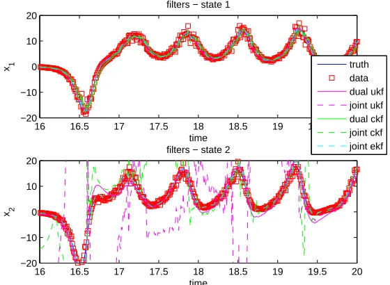
Figure 2.1 Top: Plot of filter estimates for x1 utilizing both joint and dual filters over all ob-servations. Bottom: Plot of filter estimates forx1utilizing both joint and dual filters over short time scale. This gives a better perspective of the methods tracking ability. 30 Figure 2.2 Plot of Parameter estimates for the dual UKF and dual CKF along with 3 standard
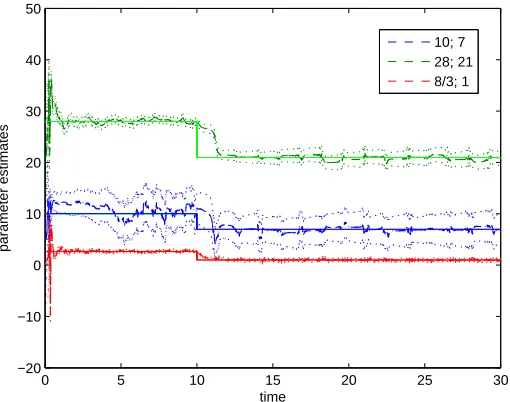
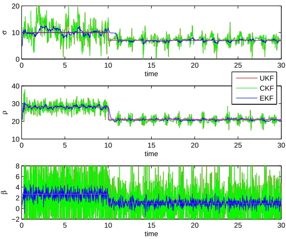
deviations (dotted) over the all observations, as well as true parameter values; green: ρblue:σ. red:β. . . 30 Figure 2.3 Plot of parameter estimates for the joint EKF, joint UKF and joint CKF over all
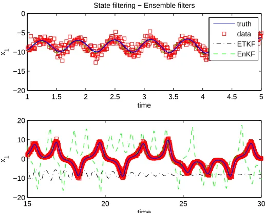
ob-servations, as well as true parameter values (purple lines). UKF and CKF obtained nearly identical results and therefore the UKF (red) is not visible. . . 31 Figure 2.4 Top: Plot of ensemble methods’ state filter estimate ofx1 for the Lorenz equations
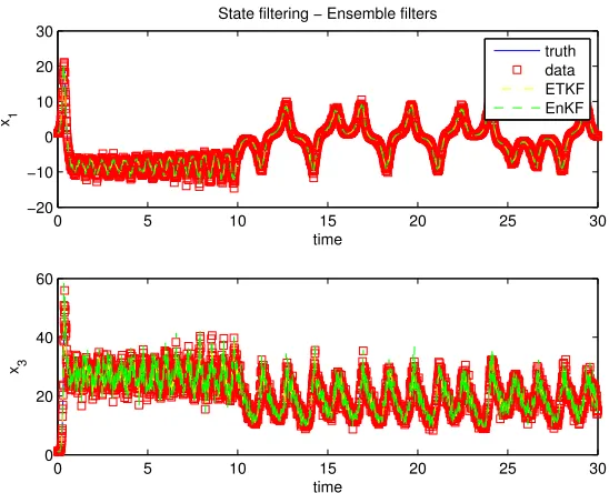
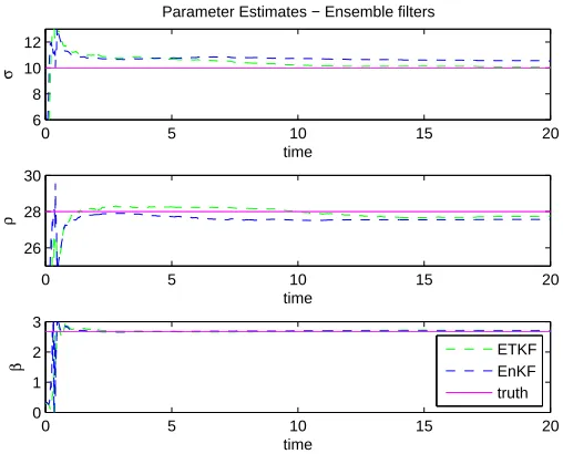
prior to parameter shift. Bottom: Plot of ensemble methods’ state filter estimate of x1for the Lorenz equations post parameter shitf. . . 33 Figure 2.5 Plot of parameter estimates for both ensemble filters over all observations. . . 33 Figure 2.6 Top: Plot of updated ensemble state filter estimates ofx1 for the Lorenz equations
over all observations. Bottom: Plot of updated ensemble state filter estimates ofx3 of the Lorenz Equations over all observations. . . 35 Figure 2.7 Plot of parameter estimates for both updated ensemble filters over all observations
along with true parameter values (purple lines). . . 35 Figure 2.8 Top: Plot of joint and dual state filter estimates for x1 over short time scale given
observations only for x1. Bottom: Plot of joint and dual state filter estimates forx2 over same short time scale given observations only forx1. . . 36 Figure 2.9 Plot of joint and dual filters’ parameter estimates given observations only forx1. . 37 Figure 2.10 Top: Plot of ensemble methods’ state filter estimates for x1 over short time scale
given observations only for x1. Bottom: Plot of ensemble methods’ state filter esti-mates forx2over same short time scale given observations only forx1. . . 38 Figure 2.11 Plot of parameter estimates using ensemble filters given observations only for x1
along with true parameter values (purple lines). . . 38 Figure 2.12 Plot of filter estimates for the number of uninfected T cells,T∗, over all the
mea-surements. . . 41 Figure 2.13 Plot of filter estimates for the number of infected T cells . . . 43 Figure 2.14 Plot of parameter estimates forλ,k andδfor all the filters; blue dashed line is the
Figure 2.15 Hemodynamic schematic of the simple model of Ursino and Lodi [28]. Arterial (red) and venous (blue) compartments are enclosed within the intracranial space (brown,Cic: intracranial compliance). Regulated variables (Ca: arterial compliance, Ra: arterial resistance) implicitly account for dynamics of hemodynamic variables (pa: extracranial arterial blood pressure,q: MCA territory arterial blood flow, pc: capillary blood pressure, pic: intracranial pressure, pv: intracranial venous blood pressure,qf: cerebrospinal fluid (CSF) formation rate,qo: CSF outflow rate) and constant hemodynamic variables (Rpv: pial venus flow resistance,Rv: cortical cere-bral venous flow resistance,Rf: CSF formation resistance,Ro: CSF outflow resis-tance,pvs: venous sinus blood pressure). Reprinted with acknowledgement to Mikio Aoi [2]. . . 45 Figure 2.16 Left: simulated data, ˆv(red), true blood flow velocity (blue), filter estimate for
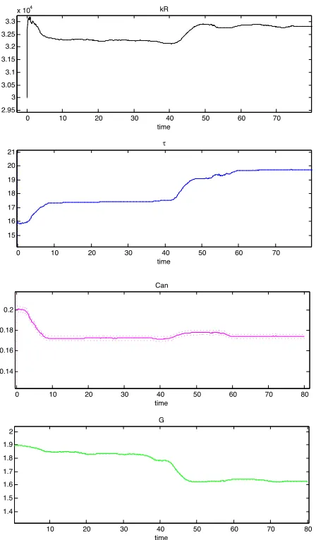
sim-ulated blood flow velocity (green), NLS estimate for simsim-ulated blood flow velocity (cyan). Bottom plot displays the simulated blood flow velocity and fits due to both methodologies over a shorter time scale. Right: Plot of hidden stateCa with added noise (red), true solution (blue), filter estimate (green), and NLS estimate (cyan). . 47 Figure 2.17 parameter estimates for 4 of the 5 parameters for the U-L autoregulation model;
(from top to bottom) 1:kR2:τ3:Can4:G . . . 48 Figure 2.18 Plot of blood flow velocity data (red), filter estimate for the blood flow velocity
(blue) and NLS model estimate for blood flow velocity (green). The NLS approach is using optimized values . . . 50
Figure 3.1 Blood flow from the left ventricle through the systemic arteries and veins to the right atrium. It is then ejected from the right ventricle and pumped through the pulmonary circulation back to the left atrium. Systemic arteries and pulmonary veins are O2 -rich, CO2-poor blood, while systemic veins and pulmonary arteries are O2poor and CO2rich. Reprinted from [6]. . . 56 Figure 3.2 Left: Typical pressure during systemic circulation. Right: Typical pressure in
pul-monary circulation. In both, the oscillations represent variations in time, not dis-tance. Reprinted with permission from [1]. . . 57 Figure 3.3 Diagram of a typical cardiac cycle. The figure shows the relationship between heart
sounds and the intraventricular pressure and volume. The top graph represents the pressures in the left ventricle and left atrium. The bottom graph shows the ventric-ular volume. Reprinted with permission from [6]. . . 58 Figure 3.4 Pressure-volume loop and four phases of the cardiac cycle. Line segments
repre-sent AC: Diastole, CD: Contraction, DF: systole, FA: relaxation. Reprinted with permission from [1]. . . 59 Figure 3.5 Branching structure of the typical vascular bed. Reprinted with permission from [1]. 60 Figure 3.6 Diagram of the pathways by which the sympathetic and parasympathetic system’s
Figure 4.1 Compartment model used for predicting HUT dynamics in the systemic circulation. The model includes five compartments representing the left heart (lh), arteries (a), and veins (v) in the upper (u) and lower (l) body. Flows are marked byq, pressures by p, volumes by V, resistors by R, compliances byC. The opening and closing of the aortic (av) and mitral (mv) vales and prevention of retrograde flow through systemic veins are modeled via pressure-varying resistors. . . 66 Figure 4.2 Ranked total sensitivities, ||∂pau/∂θ||˜ 2, for CV model. Ranked from most to least
sensitive. 1:Emax 2:Emin 3:Cau 4:Raup5:Rvl6:Cal 7:Cvu 8:Cvl 9:TR 10:Ral 11: Ralp12:Vun,lh . . . 71 Figure 4.3 Plot of Nonlinear Least Squares and Ensemble Transform Kalman Filter fit to
Pres-sure data,pau, and Residual distributions. . . 79 Figure 4.4 Plots of ETKF results of unobserved states as described; upper left: pal, lower left:
pvl, upper right:Vlv, lower right:pvu. . . 80 Figure 4.5 Absolute value of residuals withσand 2σfrom the filter fit for pau. Assuming the
residuals are normally distributed, 68% of the data should fall under the 1σ line while 95% should fall under the 2σline. . . 81 Figure 4.6 NLS estimate forRaupalong with confidence bounds derived through DRAM
com-pared to ETKF estimate forRaupwith confidence intervals in log scale. . . 81 Figure 4.7 NLS estimate forEminalong with confidence bounds derived through DRAM
com-pared to ETKF estimate forEminwith confidence intervals in log scale. . . 82
Figure 5.1 Schematic representation illustrating the interplay between absorption, distribution, binding, and elimination (excretion and metabolism) kinetics as well as dynamics of a drug. . . 92 Figure 5.2 Illustration of the absorption, distribution, and transport of a drug through the
vari-ous barriers and membranes to its target. . . 94
Figure 6.1 Diagram representing the two compartment model. Absorption compartment,Aa, represents the gut. Drug is taken into the absorption compartment and is transported into the central compartment at rate ka. The drug can diffuse into the peripheral compartmentAperipheralat a ratek12and can diffuse back at ratek21. The drug will be eliminated from the body at rateke. . . 108 Figure 6.2 Top: Population PK model fit for 16 subjects concentration profiles in log-space
for concentration. Base model fit utilizes a 2-compartment oral absorption model with log-additive error. Bottom: Individual predictions vs. individual concentra-tions along with unity line (blue). Unity line represents the ideal situation where the model perfectly predicts the observations. . . 109 Figure 6.3 Left: Population PK model fit utilizing EKF for 16 subjects concentration profiles
Figure 6.4 Left: Plasma concentration profile for Subject 1 including data, initial 2-compartment model (ODE), EKF absorption rate tracking model (EKF), UKF absorption rate tracking model (UKF), and Wiebull absorption 2-compartment model (Wiebull); prediction intervals are presented for the UKF calculated as ˆyj|j−1±
p
R(j|j−1)Right: EKF and UKF filter predictions for Subject 1 along with prediction intervals for each filter. . . 112 Figure 6.5 Absorption rate profiles, ka, for Wiebull, EKF, and UKF models. This figure
dis-plays the temporal dynamics of the absorption rate of QD dose metformin for each individual. . . 112 Figure 6.6 Left: Plots of the fraction yet to be absorbed of metformin utilizing the EKF, UKF,
and Wiebull ODE model. Right: Mass balance of drug over time for the EKF, UKF, and constrained EKF solutions. . . 113 Figure 6.7 Absorption rate profiles,ka, for Wiebull and constrained EKF models. . . 114 Figure 6.8 Top: Population PK model fit for 16 subjects concentration profiles in log-space
Chapter 1
Introduction, Motivation, and Outline
A model is a set of equations constructed to represent the interactions of various variables within a biological or physical process. Often, the model only incorporates the pertinent information for the system of interest, and will exclude variables or processes which are deemed insignificant or have little impact. Even if a model fully encapsulates the real world process, it may rely on initial conditions, boundary conditions, or parameters which are difficult to prescribe to high accuracy and precision [2].
The type of model constructed will also have an effect on the outcome and utility. Empirical mod-els are created purely based upon observations rather than mathematically describable relationships of the system. Mechanistic models are constructed as representative abstractions of the underlying pro-cesses and are often compared to data for prediction purposes [8]. Mechanistic models are governed by physical relations and laws, and therefore often have less parameters than empirical models. Within this framework, models can then be classified as deterministic, thus having exact determinability, or stochastic, incorporating a level of statistical uncertainty within the predictions.
Resolving a model, we obtain a solution or single realization of the process outcome, out of a possible infinite number of realizations, without any understanding of the uncertainty associated with the model solution. The solution techniques introduce another level of uncertainty as numerical techniques have finite accuracy and precision. Other difficulties arise due to the size, complexity, and nonlinearity of the models, along with number of parameters [1].
In addition to the model, measurements from the system are collected at temporal and spatial lo-cations. The measurements, themselves, introduce another element of uncertainty as sampling history, sampling equipment precision, and environmental conditions all introduce errors [9]. The computation of the model solution conditioned on these observed measurements defines the data assimilation or in-verse problem which will be the focus for the remainder of this study. The inin-verse problem is defined as calculating the optimal parameter values to obtain the best possible fit of the model to a specified data.
variability associated with the model solution due to the measurements and their collection, the model parameters, and the model assumptions may not fully represen the governing process [9], therefore the probability density function (pdf) of the model is considered. The pdf of the model can be used to extract information on the most likely estimate of the model state and its uncertainty [2].
For this thesis, the models of interest can be formulated as systems of ordinary differential equa-tions (ODE), or soluequa-tions thereof [7]. Applying noise to the state space of the model alters the model framework from an ODE to a stochastic differential equation (SDE). This allows the model to account for the uncertainty associated with missing processes not considered, numerical techniques, and model parameters. Shifting to the SDE approach, then, allows the model to be represented by a probability density. While a class of linear SDEs possess analytical solutions [6], as well as optimal numerical so-lutions (Kalman filters) [5], many models are nonlinear and the solution for SDEs of this type require numerical methods.
The focus of this thesis will be on utilizing nonlinear filtering methodologies to quantify system dynamics along with its utilization within the inverse framework. Few studies are explicitly concerned with using filtering techniques for parameter estimation [4], the main purpose of this study is to illustrate its novelty and utility not only for uncertainty quantification of model dynamics, but its application to parameter estimation in general.
This thesis will continue as follows. Chapter 2 will cover a multitude of nonlinear filtering meth-ods and their applications to a wide range of parameter estimation problems primarily within biological systems. A comprehensive comparison is carried out which highlights each filter’s strengths and weak-nesses on varying classes of problems.
Chapter 3 presents general background on human physiology of the cardiovascular system in gen-eral, as well as autonomic regulation. This biological background serves as motivation for the modeling done in Chapter 4.
Chapter 4 utilizes the biological background of Chapter 3 to construct a model to describe the baroreceptor and the body’s regulation of blood pressure and heart rate during head-up tilt. The general model is derived and filtering is used to understand the control systems. The results are compared to alternate methods of modeling the control along with their respective uncertainties.
Chapter 5 presents a general background on pharmacokinetics and dynamics. This will provide the foundation for Chapter 6.
Chapter 6 provides a methodology for solving inverse problems for repeated measures or population studies and its application is shown in a population pharmacokinetic study of metformin.
REFERENCES
[1] Ellwein, L.M. Cardiovascular and Respiratory Regulation, Modeling and Parameter Estimation. PhD thesis, North Carolina State University, 2008.
[2] Evensen, G. Data Assimilation: The Ensemble Kalman Filter. New York: Springer, 2009.
[3] Gabrielsson, J. and Weiner, D. Pharmacokinetic and Pharmacodynamic Data Analysis: Concepts and Applications. Stockholm, Sweden: Swedish Pharmaceutical Press, 2006.
[4] Haykin, S. Kalman Filtering and Neural Networks. New York: John Wiley and Sons, Inc., 2001.
[5] Kalman, R.E. ”A New Approach to Linear Filtering and Prediction Problems.” ASME J. Basic Engineering. Vol. 82, 1960, Pgs. 34-45.
[6] Klebaner, F.C. Introduction to Stochastic Calculus with Applications. London, UK: Imperial Col-lege Press, 2005.
[7] Overgaard, R.V., Jonsson, N., Tornoe, C.W., and Madsen, H. ”Nonlinear Mixed-Effects Mod-els with Stochastic Differential Equations: Implementation of an Estimation Algorithm.” Journal of Pharmacokinetics and Pharmacodynamics. Vol. 32, No. 1, 2005, Pgs. 85-107.
[8] Riviere, J. Comparative Pharmacokinetics Principles, Techniques, and Applications. West Sussex, UK: John Wiley, and Sons, 2011.
[9] Tornoe, C.W., Overgaard, R.V., Agerso, H., Nielsen, H.A., Madsen, H., and Jonsson, E.N. ”Stochas-tic Differential Equations in NONMEM: Implementation, Application and Comparison with Ordi-nary Differential Equations.” Pharmaceutical Research. Vol. 22, No. 8, 2005, Pgs.1247-1258.
Chapter 2
Nonlinear Filtering Methodologies for
Parameter Estimation
2.1
Introduction
For many problems in science, the estimation of the state of a system given a set of system observations is ubiquitous. Given that mathematical models approximate the true dynamics of the underlying system and that any measurement of the system dynamics is noisy, we wish to find an optimal method to combine these to get more accurate estimates of the state of the system, and any model parameters. An optimal method to do this is to use the Bayes filter; however, the Bayes filter can rarely be solved analytically, and numerical approximation is often intractable, except for a small set of restrictive cases [3].
One solution to the Bayes filter is the celebrated Kalman filter [27]. Assuming that the model is linear and that the errors in both the model and the observations are Gaussian, the Bayes filter simplifies to the Kalman filter, which calculates the optimal state of the system by taking a weighted average of the probability distribution from the model and the probability distribution from the measurement. It is deterministic in nature and characterizes the entire optimal estimate through the propagation of the mean and covariance of the estimate at each step. However, if these restrictive assumptions do not hold and the model dynamics are nonlinear or the noise distributions are non-Gaussian, the Kalman filter fails. Several variants of the Kalman filter have been developed to overcome these shortcomings.
12, 9, 19].
Another approach to handle the nonlinear model dynamics is via a statistical linearization [7]. In-stead of linearizing the model dynamics, we perform a linearization of the distribution itself by carefully choosing a set of sigma points that characterize the distribution and capture the important features. By propagating these points through the unscented transform, we get an accurate representation of the pos-terior distribution. This is done for both the model and observations, and the resulting distributions are used in the classical Kalman filter equations. This approach still assumes Gaussian distributions and is known as the Unscented Kalman Filter (UKF) [7, 14, 11, 26, 38].
The last of the deterministic approaches to be discussed is the Cubature Kalman filter [3]. It is de-rived by applying the Gaussian distribution to the Bayes filter for any nonlinear function and exploiting the properties of the highly efficient cubature numerical integration technique for the multi-dimensional integral given in the Bayes filter. Much like the Unscented Kalman Filter, this method requires the cal-culation of cubature points to characterize the integrals, which are used to calculate the distributions more accurately, and finally used in the classical Kalman filter equations.
Another set of approaches has been derived by using sampling techniques, as opposed to deter-ministic methodologies, to characterize the distributions. These sampling based methods sample a large number of points from the assumed distribution and propagate them forward. The characterization of the distribution is now done using straightforward calculations of the mean and variance of these samples. The accuracy of these sample based approximate methods depends on the sampling as opposed to the previous approaches which relied upon the accuracy of the linearizations or the numerical integration. There are two types of these methods we will discuss, the Ensemble Kalman filter (EnKF) and the En-semble Transform Kalman Filter (ETKF), though many other methods exist. For example, we refer the interested reader to [1, 6, 9, 10, 13] for more information on these methods and others.
For this study, since the systems dealt with will change sequentially in time, we shall focus our efforts on state-space models using discrete time. Therefore, difference equations shall mainly be presented to describe the dynamics of a system over time. This discrete formulation shall be used as measurements are collected at discrete times in application and the modeling framework can easily be extended to continuous time.
2.2
Background and Derivation
2.2.1 Bayes Filter
The Bayes filter is an optimal method to combine a model along with measurements to get the best estimate of the state of the system, and the model parameters.
We start by defining the state-space representation as follows:
xi+1= f(i,xi,ui, θ)+wi (2.1) yi+1=h(i+1,xi+1,ui+1, θ)+vi+1, (2.2)
wherexi+1 <nx andyi+1<ny are the model state and measurement, respectively,wiandvi+1 are as-sumed to be independent and identically distributed (i.i.d.) noise processes with zero means and covari-ancesQiandRi+1,ui <nu is an exogenous control, andθdenote the model parameters. The functions
f andhare assumed to be nonlinear in the state and observations.
The objective is to use the measurements,y1:i, up to timei, to give an understanding of the state xi. This requires calculating the distribution, p(xi|y1:i), assuming that the initial distribution p(x0|y0) = p(x0), which is just the distribution of the state without any observations at the current time, known as the prior. Given the initial distribution, p(xi|y1:i) can be calculated in two steps: a prediction and an update.
Assuming time starts ati−1, withp(xi−1|y1:i−1), the prediction step involves using the model to calcu-late the prior probability density function (pdf) of the state at timeiby using the Chapman-Kolmogorov equation [5]
p(xi|y1:i−1)=
Z
p(xi|xi−1)p(xi−1|y1:i−1)dxi−1, (2.3)
which utilizes the fact thatp(xi,xi−1|y1:i−1)= p(xi|xi−1) since the model is a first order Markov process. The pdf p(xi|xi−1) is given by the state-space model (2.1) with statistics governed bywi.
Now given a measurementyibecomes available at timei, Bayes’ rule is applied to update the prior estimate and get our posterior
p(xi|y1:i)=
p(yi|xi)p(xi,y1:i−1) p(yi,y1:i−1)
, (2.4)
wherep(yi,y1:i−1)=
R
p(yi,xi)p(xi|y1:i−1)dxi.
The posterior is dependent upon the likelihood function which is defined by the measurement equa-tion (2.2), with statistics given byvi+1. Hence, the posterior updates the prior given a measurement to get the density at the current state [5] and the Bayes filter is simply a recursion relationship between (2.3) and (2.4).
obtained one at a time; when the number of time steps increases, the dimensionality of the full posterior distribution also increases leading to computationally intractable calculations [27].
2.2.2 The Kalman Filter
Assuming linear dynamics and Gaussian noise processes, the Bayes filter simplifies to the Kalman filter. Utilizing the work of Majda and Harlim [19], the Kalman filter is derived as follows. Operating with Gaussian distributions, the entire optimal estimate can be characterized through the propagation of the mean and covariance. Lettingxi+1|ibe the state at timei+1 given the state at timei, ˆxi+1|idenotes the mean of the prior distribution, andPxi+1|i the covariance of the prior distribution, the state space can be formulated as:
xi+1|i= F xi|i+wi (2.5) yi+1= H xi+1+vi+1, (2.6)
wherewiandvi+1are normally distributed with mean 0 and covariances, QandR, respectively, and F andHare matrix operators. For simplification, we shall use the following notation to describe distribu-tions,wi ∼ N(0,Q) andvi+1 ∼ N(0,R) where∼ denotes distributed andN(0,R) denotes normal with mean 0 and covarianceR. This givesp(xi+1)∼N( ˆxi+1|i,Pxi+1|i) with
Pxi+1|i =
(xi+1−xˆi+1|i)(xi+1−xˆi+1|i)T, (2.7)
wherehAidenotes the mean ofA.
Substituting (2.5) into (2.7), the following equation for the covariance prediction can be obtained,
Pxi+1|i =
(F xi|i+wi+1−Fxˆi|i)(F xi|i+wi+1−Fxˆi|i)T (2.8)
=F
(xi|i−xˆi|i)(xi|i−xˆi|i)TFT +Q= FPxi|iF T+Q.
(2.9)
Assuming Gaussian distributions, the distributions become
p(xi+1)∝e
−1
2(x−xˆi+1|i)T(Pxi+1|i)
−1(x−xˆ
i+1|i) (2.10) p(yi+1|xi+1)∝e−
1
2(yi+1−H x) TR−1(y
i+1−H x). (2.11)
By applying Bayes formula, p(xi+1|yi+1) ∝ p(xi+1)p(yi+1|xi+1), where ∝ denotes proportionality, the posterior can be written as
p(xi+1|yi+1)∝e− 1
2J[x], (2.12)
whereJ[x]=(x−xiˆ+1|i)T(Pxi+1|i)
−1(x−xiˆ
+1|i)+(yi+1−H x)TR−1(yi+1−H x).
as minimizingJ[x]. The necessary condition forJ[x] to be minimized is
dJ dx =P
−1
xi+1|i(x−xiˆ+1|i)+(x−xiˆ+1|i) T
P−x1 i+1|i −H
T
R−1(yi+1−H x)+(yi+1−H x)TR−1(−H) (2.13)
=2(Pxi+1|i)
−1(x−xˆ
i+1|i)−2HTR−1(yi+1−H x)=0, (2.14)
which implies
(Pxi+1|i)
−1(x−xiˆ
+1|i)=HTR−1(yi+1−H x). Isolating the dependent variablexyields
(P−xi1+1|i +H T
R−1H)x=P−x1
i+1|ixiˆ+1|i+H T
R−1yi+1.
Adding and subtractingHTR−1Hxˆi+1|i, the inverse of the leading term (P−xi1+1|i +H
TR−1H) is multiplied
through to obtain
ˆ
xi+1|i+1 =(Px−i1+1|i +H
TR−1H)−1P−1
xi+1|ixˆi+1|i+(P
−1 xi+1|i+H
TR−1H)−1HTR−1y i+1+
(P−xi1+1|i+H T
R−1H)−1HTR−1Hxˆi+1|i−(P−xi1+1|i+H T
R−1H)−1HTR−1Hxˆi+1|i,
where ˆxi+1|i+1is the mean of the posterior distribution. Rearranging the terms gives
ˆ
xi+1|i+1 =(P−xi1+1|i+H T
R−1H)−1P−x1
i+1|ixiˆ+1|i+(P
−1 xi+1|i +H
T
R−1H)−1HTR−1Hxiˆ+1|i+ (P−xi1+1|i +H
T
R−1H)−1HTR−1(yi+1−Hxiˆ+1|i).
Adding the ˆxi+1|iterms together and simplifying leads to
ˆ
xi+1|i+1 = xiˆ+1|i+Ki+1(yi+1−Hxiˆ+1|i), (2.15)
whereKi+1is defined as
Ki+1=(P−xi1+1|i+H T
R−1H)−1HTR−1, (2.16)
also known as the Kalman gain. Equation (2.15) is the mean update for the state. A more common expression for the Kalman gain can be obtained by multiplyingKi+1 by (HPxi+1|iH
T +R)(HP xi+1|iH
T +
R)−1;
Ki+1=(P−xi1+1|i +H
TR−1H)−1HTR−1(HP xi+1|iH
T+R)(HP xi+1|iH
T +R)−1. (2.17)
MultiplyingRby (Pxi+1|iH T)−1Px
i+1|iH
T in (HPx i+1|iH
T +R)(HPx i+1|iH
T +R)−1gives
(HPxi+1|iH
T+R)(HP xi+1|iH
T+R)−1=(HP xi+1|iH
T+R(P xi+1|iH
T)−1P xi+1|iH
T)(HP xi+1|iH
Substituting (2.18) into (2.17) and expanding yields
Ki+1=(P−xi1+1|i +H T
R−1H)−1
HTR−1HPxi+1|iH T +
HT(Pxi+1|iH T
)−1Pxi+1|iH T
(HPxi+1|iH T +
R)−1. (2.19)
Substituting (Pxi+1|iH
T)−1 =(HT)−1P−1
xi+1|i into (2.19) yields
Ki+1=(P−xi1+1|i +H T
R−1H)−1
HTR−1H(Pxi+1|iH T
)+HT(HT)−1P−x1
i+1|i(Pxi+1|iH T
)
(HPxi+1|iH T+
R)−1.
Rearranging terms results in
Ki+1=(P−xi1+1|i +H
TR−1H)−1
(HTR−1H+P−x1
i+1|i)(Pxi+1|iH T)
(HPxi+1|iH
T +R)−1.
Simplifying, we finally arrive at
Ki+1=Pxi+1|iH T
HPxi+1|iH T+
R−1,
(2.20)
which is the more common expression for the Kalman Gain. By substituting (2.15) into the covariance formula,
(xi+1−xˆi+1|i+1)(xi+1−xˆi+1|i+1)T, (2.21)
we obtain
(xi+1−xiˆ+1|i+1)= xi+1−xiˆ+1|i−Ki+1(yi+1−H xi+1−H( ˆxi+1|i−xi+1)).
Letei+1|i+1 = xi+1−xˆi+1|i+1be the error between the true state and the estimated state. Using the output equation (2.6) leads to
ei+1|i+1=(I−Ki+1H)ei+1|i−Ki+1(H xi+1+vi+1−H xi+1) (2.22) ei+1|i+1=(I−Ki+1H)ei+1|i−Ki+1vi+1. (2.23)
Using (2.23), the covariance update is given by
ei+1|i+1eTi+1|i+1
=
(I−Ki+1H)ei+1|ieTi+1|i(I−Ki+1H)T+Ki+1RKiT+1 (2.24)
ei+1|i+1eTi+1|i+1
=
(I−Ki+1H)ei+1|ieiT+1|i−(I−Ki+1H)ei+1|ieTi+1|i(Ki+1H)T+Ki+1RKiT+1. (2.25)
Substituting (2.16) into (I−Ki+1H) and simplifying results in
(I−Ki+1H)=(P−xi1+1|i +H T
R−1H)−1(P−xi1+1|i+H T
R−1H)−(P−xi1+1|i+H T
R−1H)−1HTR−1H (2.26)
=(P−xi1+1|i +H T
R−1H)−1P−x1
Applying the definition of the covariance,
ei+1|ieTi+1|i= Pxi+1|i, along with substituting (2.27) and ex-panding (2.25) yields
ei+1|i+1eTi+1|i+1
=
(I−Ki+1H)Pxi+1|i − (P
−1 xi+1|i+H
T
R−1H)−1P−x1 i+1|i
Pxi+1|iH T
KTi+1+Ki+1RKiT+1
=(I−Ki+1H)Pxi+1|i −(P
−1 xi+1|i +H
TR−1H)−1HTKT i+1
+ (P−xi1+1|i+H T
R−1H)−1HTR−1
RKiT+1
=(I−Ki+1H)Pxi+1|i −(P
−1 xi+1|i +H
T
R−1H)−1HTKiT+1
+(P−xi1+1|i +H
TR−1H)−1HTKT i+1.
Simplifying, the covariance update becomes
Pxi+1|i+1 =(I−Ki+1H)Pxi+1|i. (2.28)
In summary, the above derivation for the Kalman filter essentially contains two steps. Prediction
ˆ
xi+1|i= F xi|i (2.29) Pxi+1|i =FPxi|iF
T+
Q (2.30)
Update
ˆ
xi+1|i+1= xiˆ+1|i+Ki+1(yi+1−Hxiˆ+1|i) (2.31)
Ki+1 =Pxi+1|iH T
HPxi+1|iH T +
R−1
(2.32) Pxi+1|i+1 =(I−Ki+1H)Pxi+1|i. (2.33)
As stated, however, this only holds if the model dynamics and observation equation are both linear and the noise processes are Gaussian. For cases when these do not hold, modifications to the Kalman filter have been developed.
2.3
Deterministic Kalman Filters
2.3.1 The Extended Kalman Filter
is derived as follows. Assuming a general nonlinear system as below:
xti+1= f(i,xti,ui, θ)+wi (2.34)
yti+1=h(i+1,xti+1,ui, θ)+vi+1, (2.35)
and assuming this system is modeled by the approximate equation
ˆ
x−i+1 = f(i,xˆi,ui, θ), (2.36)
subtracting (2.36) from (2.34) obtains
xti+1−xˆ−i+1= f(i,xti,ui, θ)− f(i,xi,ˆ ui, θ)+wi. (2.37)
A Taylor expansion can be performed to approximate the system
f(x)= f(x0)+ d f
dx(x0)(x−x0)+ 1
2(x−x0) TFxx(x
0)(x−x0)T +O||x−x0||3,
whereFxxis used to denote the second derivative, or Hessian matrix for multiple dimensions. Applying this expansion to the original system leads to
xti+1−xˆ−i+1= f(i,xi,ˆ ui, θ)+d f dx( ˆxi)(x
t i−xi)ˆ +
1 2(x
t
i−xi)Fxx( ˆˆ xi)(x t i−xi)ˆ
T+
O||x−x30||
−f(i,xi,ˆ ui, θ)+wi.
Squaring both sides and taking the expected value leads to the following equation
Pxi+1|i =Fx( ˆxi)E[(x t
i−xˆi)(xit−xˆi)] T
Fx( ˆxi)T+ 1
2Fx( ˆxi)E[(x t i−xˆi)(x
t i−xˆi)
T
]FTxx( ˆxi)E[(x t i−xˆi)]
+1
4E[(x t i−xi)(xˆ
t i−xi)ˆ
T]FxxFT xxE[(x
t i−xi)(xˆ
t i−xi)ˆ
T]+...+Q,
which simplifies by discarding the moments of third or higher order
Pxi+1|i ≈ Fx( ˆxi)Pxi|iFx( ˆxi) T +Q,
(2.38)
whereFx( ˆxi) = ∂ f(i,x)
∂x |x=xˆi is the Jacobian, Qis the model error covariance, andPxi+1|i is the predicted error covariance.
Applying the same procedure to the nonlinear observation equationh, we utilize a linearization of the observation equation to be used in the update as follows
Hi+1=
∂h(i,x) ∂x |x=xˆ
−
i+1.
filter. While the initial state estimation portion of the algorithm is unchanged, these Jacobians are utilized in the initial covariance estimation and in the estimation update for both the covariance and the state, through the gain. Though utilizing the same procedure as the Kalman filter, the extended Kalman filter is sub-optimal for nonlinear problems, and reduces to the Kalman filter for linear problems.
The algorithm for the extended Kalman filter is summarized as follows:
Initialize: fori=0 ˆ
x0=E[x0]
P0=E[(x0−E[x0])(x0−E[x0])T] algorithm: for i=1,2,3,...
State Estimation
ˆ
x−i = f(i,xiˆ−1) Covariance Estimation
P−i =Fi,i−1Pi−1FTi,i−1+Qi−1
whereFis the linearization of the model w.r.t. the state
Fi,i−1=
∂f(i,x) ∂x |x=xˆi−1 Kalman Gain Matrix
K=P−i HiT
HiP−iH T i +Ri
−1
whereHis the linearization of the observation w.r.t. the state
Hi = ∂h(i,x) ∂x |x=xˆ−
i
State Estimation Update
ˆ
xi = xˆ−i +K
yi−h(i,xˆ−i)
Covariance Estimation Update
Pi =I−KHiP−i
the approximation of the error statistics by the linearized model, since a Gaussian distribution cannot be guaranteed once propagated through a nonlinear operator.
To increase the accuracy of nonlinear models, another Kalman filter has been constructed that better preserves the distribution statistics as it passes through the nonlinearities. Unlike the EKF, this new filter maintains at least second order accuracy for all distributions, and at least third order accuracy for Gaussian distributions [14].
2.3.2 The Unscented Kalman Filter
The unscented Kalman filter addresses the shortcomings of the EKF through the ’unscented transfor-mation.’ Following the work by Haykin [14], the unscented Kalman filter is derived assuming the errors are Gaussian random variables (GRV). Instead of using a linear approximation to the nonlinear model, a set of sample points is constructed which will completely capture the true mean and covariance of the GRV, and once propagated through the nonlinear model, will capture the posterior mean and covariance to 3rd order for any nonlinearity [38]. The advantages of the unscented Kalman filter are not just the increase of accuracy, but also the decrease in complexity by not requiring the calculation of a derivative, or Jacobian. To better understand, we shall explain the unscented transformation.
The unscented transformation (UT) is a method used to calculate the statistics of a random variable which undergoes a nonlinear transformation [11]. Assuming thatxis a random variable with dimension L, which has mean ˆx and covariance, Px, this random variable gets propagated through a nonlinear function,y=g(x). To calculate the statistics ofy, a matrixχis formed of 2L+1 sigma vectorsχi. This matrixχis constructed as follows,
χ=
ˆ
x, x1ˆ 1xL+ p(L+λ)Px
L, ˆx11xL−
p
(L+λ)Px L
,
(2.39)
where ˆx is a column vector, ˆx11xL is a matrix of the column vector ˆx, and
√
(L+λ)PxL is an LxL matrix. The corresponding weights (Wi) for the sigma vectors are as follows
W0(m) = λ
(L+λ) (2.40)
W0(c) = λ
(L+λ) +(1−α
2+β) (2.41)
Wi(m) =Wi(c)= 1
2(L+λ) i=1, ...,2L, (2.42)
tuning parameter,κ, is a secondary scaling parameter which is optimally set to 3−L[14]. Lastly,βis used to incorporate prior knowledge of the distribution ofx(for Gaussian distributions,β=2 is optimal) [38]. From our matrix of sigma points (2.39), √(L+λ)Px
iis theith row of the matrix square root [38]. The sigma vectors are then propagated through the nonlinear function accordingly,
yi=g(χi), i=0, ...,2L, (2.43)
with the mean and covariance ofybeing approximated using a weighted sample mean and covariance of the posterior sigma points,
ˆ y≈
2L
X
i=0
Wi(m)yi (2.44)
Py ≈ 2L
X
i=0
Wi(c) yi−yˆyi−yˆ T.
(2.45)
Gaussian noise),
Initialize: fort=0 ˆ
x0=E[x0]
P0=E[(x0−E[x0])(x0−E[x0])T] algorithm: for t=1,2,3,...
Calculate Sigma Points χt−1=x,ˆ xˆ+
p
(L+λ)Pt−1L, xˆ−
p
(L+λ)Pt−1L
time-update equations χ∗
t,t−1=F(χt−1,ut,wt)
whereutis an exogenous input andwtare parameters
ˆ x−t =
2L
X
i=0
Wi(m)χ∗i,t|t−1
P−t = 2L
X
i=0
Wi(c) χ∗i,t|t−1−xˆ−tχ∗
i,t|t−1−xˆ
−
t
T +
Q
time-update equations for observation: augment sigma points
χt|t−1=χ∗0,t|t−1 χ
∗
0,t|t−1+
q
(L+λ)P−t
L, xˆ−
q
(L+λ)P−t
L
Yt|t−1=g(χt,t−1)
ˆ y−t =
2L
X
i=0
Wi(m)Yi,t|t−1
measurement-update equations
Pyˆtyˆt = 2L
X
i=0
Wi(c) Yi,t|t−1−yˆ−t
Yi,t|t−1−yˆ−t
T+
R
Pxtyt = 2L
X
i=0
Wi(c) χi,t|t−1−xˆ−t
Yi,t|t−1−yˆ−t
T
Kt =PxtytP
−1 ˆ ytyˆt ˆ
xt = xˆ−t +Kt yt−yˆ−t
Pt =P−t −KtPˆytyˆtK T t
whereQis the process noise covariance andRis the measurement noise covariance.
Also, a more general form of the UKF is also available, which does not assume additive noise, but prop-agates the measurement and process covariance through the nonlinear function. These extensions can be found in most of our referenced materials [14, 11, 26, 38, 30].
2.3.3 The Cubature Kalman Filter
Similar to the previous deterministic filters, the cubature Kalman filter (CKF) relies upon an approxima-tion of the nonlinear funcapproxima-tion and is derived following the work of Arasaratnam [3]. However, unlike the previous methods, the CKF closely follows the Bayes filter theory and takes advantage of the assumption of a normal distribution using numerical integration techniques to calculate the time and measurement updates. This underlying assumption of a Gaussian distribution for the predictive density and the mea-surement density is central as it leads to a Gaussian posterior distribution [3].
The prediction step, or time update, is focused on calculating the mean ˆxi+1|i and covariancePi+1|i of the predictive density
ˆ
xi+1|i =E[xi+1|u1:i,y1:i]. (2.46) Substituting the model (2.63) into (2.46), obtains
ˆ
xi+1|i= E[f(i,xi,ui, θ)+wi|u1:i,y1:i]=E[f(i,xi,ui, θ)|u1:i,y1:i].
This result follows because wi is assumed to be a zero-mean noise process that is uncorrelated with previous measurements. The expectation becomes
ˆ xi+1|i =
Z
<nx
f(i,xi,ui, θ)p(xi|u1:i,y1:i)dxi
=
Z
<nx
f(i,xi,ui, θ)(xi; ˆxi|i,Pi|i)dxi,
where(.;., .) is standard notation for a Gaussian density. Following the same procedure, the predictive
covariance is
Pi+1|i= E[ xi+1−xˆi+1|i xi+1−xˆi+1|i T
|u1:i,y1:i].
Again, substituting (2.63) in forxi+1, using f(xi) for shorthand to represent f(i,xi,ui, θ) leads to
Pi+1|i =E f(xi)+wi−xˆi+1|i f(xi)+wi−xˆi+1|i T
|u1:i,y1:i
=E
f(xi)f(xi)T + f(xi)wTi − f(xi) ˆxTi+1|i+wif(xi)T
+wiwTi −wixˆiT+1|i−xiˆ+1|if(xi)T −xiˆ+1|iwTi +xiˆ+1|ixˆTi+1|i|u1:i,y1:i
Assuming thatwi is independent of both f(xi) and ˆxi+1|i, we can useE[xy] = E[x]E[y] andE[E[x]] =
E[x]. Knowing thatwi∼ N(0,Q) and ˆxi+1|i= E[f(xi)|u1:i,y1:i], the previous expression simplifies to be
Pi+1|i =Ef(xi)f(xi)T − f(xi) ˆxTi+1|i+wiwTi −xiˆ+1|if(xi)T+xiˆ+1|ixˆTi+1|i|u1:i,y1:i
=E
f(xi)f(xi)T
−E
f(xi) ˆxTi+1|i+
E
wiwTi
−E
f(xi) ˆxTi+1|i+
E
ˆ
xi+1|ixˆTi+1|i.
Further simplifying−2E
f(xi) ˆxTi+1|i+
E
ˆ
xi+1|ixˆTi+1|iusingEf(xi)ExˆTi+1|i= xˆi+1|ixˆTi+1|i, gives
Pi+1|i =
Z
<nx
f(i,xi,ui, θ)f(i,xi,ui, θ)T(xi; ˆxi|i,Pi|i)dxi−xiˆ+1|ixˆTi+1|i+Qi.
For the measurement update, assuming measurement errors are from Gaussian distributions, the likelihood function can be written as
p(yi+1|u1:i,y1:i)=(yi+1; ˆyi+1,Pyy,i+1|i),
where the measurement prediction, calculated using the same procedure as the prediction step, is
ˆ yi+1 =
Z
<nx
h(i+1,xi+1,ui+1, θ)(xi+1; ˆxi+1|i,Pi+1|i)dxi+1.
The associated covariance, calculated using the same procedure as the prediction step, is given by
Pyy,i+1|i =
Z
<nx
h(xi+1)h(xi+1)T×(xi+1; ˆxi+1|i,Pi+1|i)dxi+1−yiˆ+1yˆTi+1+Ri.
Therefore, the joint conditional Gaussian density of the state and measurement is given by
p
[xTi+1yTi+1]T|y1:i,u1:i
= ˆ xi+1|i
ˆ yi+1
,
Pi+1|i Pxy,i+1|i PTxy,i+1|i Pyy,i+1|i
! ,
where the cross covariance is calculated as follows, substituting (2.64),
Pxy,i+1|i =E(xi+1−xiˆ+1|i)(yi+1−yiˆ+1)
=E
(xi+1−xiˆ+1|i)(h(xi+1)+vi+1−yiˆ+1),
E(xi+1|y1:i,u1:i)=xiˆ+1|iandE(h(xi+1)|y1:i,u1:i)=yiˆ+1, we obtain
Pxy,i+1|i =E xi+1h(xi+1)T+xi+1vTi+1−xi+1yˆ T
i+1−xiˆ+1|ih(xi+1) T
−xiˆ+1|ivTi+1+xiˆ+1|iyiˆ+1
=E xi+1h(xi+1)T−E xi+1yˆTi+1
−E xˆi+1|ih(xi+1)T+E xˆi+1|iyˆi+1
=Z
<nx
xi+1h(i+1,xi+1,ui+1, θ)T(xi+1; ˆxi+1|i,Pi+1|i)dxi+1−xiˆ+1|iyiˆ+1.
Given a new measurementyi+1, the posterior densityp(xi+1|y1:i+1,u1:1+i) is calculated from the Bayesian filter, resulting in
p(xi+1|y1:i+1,u1:i+1)=(xi+1; ˆxi+1|i+1,Pi+1|i+1), (2.47) where
ˆ
xi+1|i+1= xˆi+1|i+Ki+1(yi+1−yˆi+1|i) (2.48)
Pi+1|i+1=Pi+1|i−Ki+1Pyy,i+1|iKiT+1 (2.49) Ki+1=Pxy,i+1|iPyy−1,i+1|i, (2.50)
which, if f(...) andh(...) are linear functions of the state, simplifies to the classical Kalman filter.
The remaining question now becomes how to calculate an integral of the form,
Z
<n
g(x)(x)dx=
Z
<n
g(x) exp(−xTx)dx.
Arasaratnam [3, 4] proposes that the best way to do this is (i) transform it into a more familiar spherical-radial integration form, and (ii) subsequently apply a third-degree spherical-spherical-radial rule .
First, a transformation must be made to change the variables from the Cartesian space x ∈nto a radiusrand directionyas follows: letx=rywithyTy=1, so thatxTx=rforr∈[0,∞) [3]. Then, the integral becomes
I(f)=
Z ∞
0
Z
Un
f(ry)rn−1exp(−r2)dσ(y)dr,
where Un is the surface of the sphere defined by Un = {y ∈ n|yTy = 1} andσ(...) is the spherical surface measure [3]. This integral can be broken up into a radial component and spherical component which can subsequently be computed numerically using a cubature rule and quadrature rule. The radial integral is given by
I=
Z ∞
0
whereS(r) is defined by the spherical integral with unit weighting functionw(y)=1,
S(r)=
Z
Un
f(ry)dσ(y).
Carrying out both computations and combining them into a third-degree spherical-radial rule, the stan-dard Gaussian weighted integral is calculated
I(f)= Z
<n
f(x)×(x; 0,I)dx≈ m
X
i=1
ωif(ξi),
where
ξi =
r
m 2[1]i ωi = 1
m, i=1,2, ...m=2n.
Here [1]i denotes a generator, where a generator u in a fully symmetric region is defined by u = (u1,u2, ...,ur,0, ...0)∈ <n withui ≥ ui+1 > 0,i= 1,2, ...(r−1). For example, [1]∈ <2is represented by the points
1 0 , 0 1 , −1 0 , 0 −1 ! ,
using the notation that [u1,u2, ...,ur]i is thei-th point from the set [u1,u2, ...,ur]. For more information on the numerical integration details, see [3, 4].
Initialize: fort=0 ˆ
x0=E[x0]
P0=E[(x0−E[x0])(x0−E[x0])T] algorithm: for t=1,2,3,...
Calculate Matrix Square Root
Pt−1|t−1=St−1|t−1StT−1|t−1
Evaluate Cubature Points: fori=1,2, ...,2nx
Xi,t−1|t−1=St−1|t−1ξi+xtˆ−1|t−1 time-update equations
Xi∗,t|t−1= f(Xi,t−1|t−1,ut−1, θ)
whereut−1is an exogenous input andθare parameters
ˆ xt|t−1=
1 2nx
2nx
X
i=1 Xi∗,t|t−1
Pt|t−1= 1 2nx
2nx
X
i=1
Xi∗,t|t−1Xi∗,Tt|t−1−xˆt|t−1xˆTt|t−1+Qt−1
time-update equations for observation: calculate matrix square root
Pt|t−1=St|t−1STt|t−1
Evaluate Cubature Points: fori=1,2, ...,2nx
Xi,t|t−1=St|t−1ξi+xtˆ|t−1 Yi,t|t−1=h(Xi,t|t−1,ut−1, θ)
measurement-update equations
ˆ yt|t−1=
1 2nx
2nx
X
i=1 Yi∗,t|t−1
Pyy,t|t−1= 1 2nx
2nx
X
i=1
Yi,t|t−1YiT,t|t−1−ytˆ|t−1yˆ T t|t−1+Rt
Pxy,t|t−1= 1 2nx
2nx
X
i=1
ωiXi,t|t−1YiT,t|t−1−xtˆ|t−1yˆ T t|t−1
Kt =Pxy,t|t−1P−yy1,t|t−1
ˆ
whereQt−1is the process noise covariance andRt is the measurement noise covariance.
It should be noted that a distinct advantage of the cubature Kalman filter over the EKF is that it does not require the calculation of derivatives. Other advantages include the lack of tuning parameters, which have been known to have a distinct impact on the effectiveness of convergence on the UKF, and 2npoints to propagate as opposed to 2n+1. The disadvantage of the cubature Kalman filter is the strict enforcement of the Gaussian distributions for the states and observations. Again, similar to the unscented Kalman filter, there are multiple variations of this algorithm for numerical purposes, including a square root implementation. For details on this, we refer the interested reader to [3].
2.4
Sampling Based Kalman Fitlers
2.4.1 Ensemble Kalman Filter
The main idea of the ensemble Kalman filter (EnKF) is to approximate the error statistics of the estimate by a set of particles sampled from the distribution. Using the work of Majda and Harlim [19], the EnKF is derived accordingly. Unlike the deterministic methods, the prior and posterior error covariances are calculated by the ensemble covariance matrices around the corresponding ensemble mean, instead of the classical covariance equations given in the linear Kalman filter. That is, the covariance is computed
Pxi+1|i = 1
N−1Ui+1|iU T
i+1|i (2.51)
Pxi+1|i+1 = 1
N−1Ui+1|i+1U T
i+1|i+1, (2.52)
where
Ui+1|i =[x1i+1|i−xiˆ+1|i;x2i+1|i−xiˆ+1|i;...;xiN+1|i−xiˆ+1|i] (2.53)
Ui+1|i+1 =[x1i+1|i+1−xiˆ+1|i+1;x 2
i+1|i+1−xiˆ+1|i+1;...;x N
i+1|i+1−xiˆ+1|i+1], (2.54) with xij+1|i being the jthparticle being propagated through the model, andxij+1|i+1is the update of each particle. With this,Nis defined to be the number of particles in which to approximate the distribution and ˆx = N−1PN
j=1x
j. From now on,U shall be defined as the ensemble perturbation matrix as it gives the deviation of each particle from the mean. The advantage of this methodology is that unlike the deterministic methods, there is no need to do an expensive calculation, such as the linearization or statistical transform, to get error statistics. In place of these, each ensemble member is integrated in time through the dynamical model.
en-semble error covariance results in
Ki+1= Pxi+1|iH T
(HPxi+1|iH T +
R)−1
=(N−1)−1UUTHT(H(N−1)−1UUTHT+R)−1
=(N−1)−1U(HU)T((N−1)−1(HU)(HU)T+R)−1.
In the above expression, and also for the remainder of this chapter, the subscript onU is omitted for simplicity.
Looking at the Kalman gain equation, it is seen that anywhere the linear operator H appears, it is coupled to the ensemble perturbation matrix;U. Due to this consequence, given a nonlinear observation functionh,HU can be replaced with the following approximation
V =
h(x1i+1)−yˆi+1;h(x2i+1)−yˆi+1;...;h(xiN+1)−yˆi+1,
where ˆyi+1is the mean of the observation function given each sample, ˆyi+1=PNj=1h(x j i+1).
Again, the need for costly calculations can be avoided by using the ensemble approximations in place of deterministic methods.
To get final estimates, the classical Kalman filter update equations are applied to each ensemble member
xij+1|i+1 =xij+1|i+Ki+1(ymi+1−h(x j
i+1|i)), (2.55) whereKi+1is defined as above, and the observation,yi+1, is perturbed accordingly
ymi+1 =yi+1+ψmi+1, (2.56)
whereψmi+1is a Gaussian random variable with mean zero and covarianceR. This perturbation is a Monte Carlo method applied to the Kalman filter formula which yields an asymptotically correct analysis error covariance estimate for large ensemble sizes [19]. In practice, to keep these perturbations unbiased, these random perturbations are generated by first randomly drawing a MxN size matrix,A, whereN is the number of particles and M is dimension of the data, and take the singular value decomposition of (N −1)−1AAT = FP
FT. Therefore, unbiased random vectors ofymt+1 are obtained, which is just the column vectors of the matrixT = ((N−1)R)12FP−
1
2 FTA[19]. Since the measurements are being perturbed, the measurement error covariance matrix can be defined to be
R=(N−1)−1EET,
by Evensen [10], and many other implementations also exist.
Initialize: fori=0 ˆ
x0= E[x0]
P0= E[(x0−E[x0])(x0−E[x0])T] algorithm: for i=1,2,3,...
State Estimation
Sample N particles from initial distribution: forj=1, ...,N
x−i j = f(i−1,xij−1)
ˆ
xi−=(N)−1 N
X
j=1 x−i j
Covariance Estimation
U=[x−i1−xˆ−i ;x−i2−xˆi−;...;x−iN−xˆ−i ] P−i =(N−1)−1UUT
Measurement Ensemble
yij=yi+ψij
Y=
y1i,y2i, ...,yNi
E=ψ1
i, ψ 2 i, ..., ψ
N i
R=(N−1)−1EET V=h(i,
x−i1)−yˆi;h(i,x−i2)−yˆi;...;h(i,x−iN)−yˆi unbiased random vectors
[F,Σ]= svd (N−1)−1EET
T = (N−1)R12
FΣ−12FTE
Kalman Gain Matrix
Ki=(N−1)−1UVT((N−1)−1VVT +R)−1 State Estimation Update
Innov=T −Y
xij= xi−j +Ki∗Innov Posterior Covariance Update
2.4.2 Ensemble Transform Kalman Filter
Just like the EnKF, the ensemble transform Kalman filter (ETKF) relies on sampling from the proposed normal distribution to obtain the error statistics. The main idea of the ETKF is to take the square root of the covariance matrix, and transform it to a space where it is more robust and well-conditioned [12, 13, 9, 19, 30].
There are multiple methods for taking the square root, the one we shall focus on from here is the ETKF as derived by Bishop [1]. The basic idea is to find a transformation matrix T; so that
Ui+1|i+1Ui+1|iT =UT and UT(UT)T =(N−1)−1Pxi+1|i+1,
wherePxi+1|i+1is the sample posterior covariance matrix as previously defined. The posterior ensemble is then generated by taking the posterior mean and adding each column vector fromU. Using the identity
AT(AAT +R)−1=(I+AT(R−1)A)−1ATR−1, (2.57)
and letting V=A and R be the measurement error covariance, The Kalman gain becomes
Ki+1=(N−1)−1U(I+(N−1)−1VTR−1V)−1VTR−1. (2.58)
Substituting (2.58) and (2.51) into the posterior covariance formula leads to
Pxi+1|i+1 =(I− U
N−1(I+(N−1)
−1VT
R−1V)−1VTR−1H)UU T
N−1. (2.59) Factoring out NU−1 from (2.59) yields
Pxi+1|i+1 = U
N−1 I− I+
VTR−1V N−1
−1V
TR−1V N−1
UT. (2.60)
Resulting in
Pxi+1|i+1 = 1
N−1U(I−(I+B)
−1B)UT,
(2.61)
whereB= VTNR−−11V. Knowing thatI−(I+B)−1B=(I+B)−1leads to
Pxi+1|i+1 =U (N−1)I+V
TR−1V−1
UT =UΣUT =U T T T
N−1U
T. (2.62)
Initialize: fori=0 ˆ
x0= E[x0]
P0= E[(x0−E[x0])(x0−E[x0])T] algorithm: for i=1,2,3,...
State Estimation
Sample N particles from initial distribution: forj=1, ...,N
x−i j = f(i−1,xij−1)
ˆ
xi−=(N)−1 N
X
j=1 x−i j
Covariance Estimation
U=[x−i1−xˆ−i ;x−i2−xˆi−;...;x−iN−xˆ−i ] P−i =(N−1)−1UUT
Measurement Ensemble
yij=yi+ψij
Y=
y1i,y2i, ...,yNi
E=ψ1
i, ψ 2 i, ..., ψ
N i
R=(N−1)−1EET V=h(i,
x−i1)−yi;ˆ h(i,x−i2)−yi;ˆ ...;h(i,x−iN)−yiˆ
SVD of (2.62)
[X,Γ]= svd (N−1)I+VTR−1V
Kalman Gain Matrix
Ki=U XΓ−1XT)VTR−1 State Estimation Update
ˆ
xi= xˆi−+Ki(yi−h( ˆx−i )) Transformation Matrix
T = √
N−1XΓ−12XT W=UT
Posterior Ensemble and Covariance
2.5
Problem Statement
Consider a state space model of the form
xi+1= f(i,xi,ui, θ)+wi (2.63) yi+1=h(i+1,xi+1,ui, θ)+vi+1, (2.64)
where f is a nonlinear function of the statexi+1<nx, andhis a nonlinear function relating the obser-vationyi+1 <nyto the state. The variableui <nu is an exogenous control,wiandvi+1are i.i.d. noise processes, andθdenote the model parameters.
The objective is to find optimal parameter estimates allowing the best fit to the data. Classically, parameter estimation is done by using an optimization technique to minimize a cost function [29]. Often, the cost function is defined as the sum of the squares of the difference between the model output, yk, and observations,yobsk , given by
J(θ)=
N
X
k=1 γk
yobsk −yk2, (2.65)
whereγkis a weighting parameter andyobsk −yk is the residual. This approach is commonly referred to as nonlinear least squares.
While few papers are explicitly concerned with the use of filtering techniques for parameter estima-tion [14], there are multiple methods which can achieve this goal. The filters previously defined were for state estimation, the optimal combination of the model predictions and observations to obtain an improved estimate of the state of the system; however, utilizing the following methodologies allows the filters to subsequently estimate parameters. The first, and most direct, is to modify the state space rep-resentation to accommodate this objective. Since the observations are assumed to be coming from the model, and optimal parameter estimates are the main focus, one method can be obtained by assuming that the parameters have zero dynamics
θi+1=θi+ri
yi+1=h(i+1,xi+1, ,ui+1, θi+1)+vi+1,