Multiple-Interval Mapping for Ordinal Traits

DOI: 10.1534/genetics.105.054619

Multiple-Interval Mapping for Ordinal Traits

Jian Li,*

_{Shengchu Wang* and Zhao-Bang Zeng*}

*Bioinformatics Research Center,‡Department of Statistics,†Department of Genetics, North Carolina State University, Raleigh, North Carolina 27695

Manuscript received December 12, 2005 Accepted for publication March 22, 2006

ABSTRACT

Many statistical methods have been developed to map multiple quantitative trait loci (QTL) in ex-perimental cross populations. Among these methods, multiple-interval mapping (MIM) can map QTL with epistasis simultaneously. However, the previous implementation of MIM is for continuously distrib-uted traits. In this study we extend MIM to ordinal traits on the basis of a threshold model. The method inherits the properties and advantages of MIM and can fit a model of multiple QTL effects and epistasis on the underlying liability score. We study a number of statistical issues associated with the method, such as the efficiency and stability of maximization and model selection. We also use computer simulation to study the performance of the method and compare it to other alternative approaches. The method has been implemented in QTL Cartographer to facilitate its general usage for QTL mapping data analysis on binary and ordinal traits.

M

for studying the genetic basis of quantitative trait variation. A number of statistical methods have been developed over the years for QTL mapping data

anal-ysis in designed experiments, such as those of Lander

and Botstein (1989), Haley and Knott (1992),

Jansen (1993), Zeng (1993, 1994), Sillanpa¨ a¨ and

Arjas(1998), and Kaoet al.(1999). However, many of

these statistical methods focus on continuous data. Ordinal traits are also common in many QTL mapping studies. These traits take values in one of several or-dered categories. In quantitative genetics, we usually use a threshold model to model the genetic basis of

binary and ordinal traits (Wright1934a,b; Falconer

1965; Falconerand Mackay1996). In this model, we

assume that the categorical observation of a binary or ordinal trait is a reflection of an underlying continu-ously distributed liability subject to a series of thresh-olds that categorize phenotypes. Effects of QTL on observed phenotypes are modeled through the liability. A number of studies have used this threshold model for QTL mapping analysis on binary and ordinal traits. Hackett and Weller (1995) and Xu and Atchley (1996) first studied a QTL mapping method for binary/ ordinal traits based on composite interval mapping

(CIM) (Zeng1994). Visscheret al. (1996) compared

the performance and statistical power of using a linear regression and a generalized linear model directly on a

binary trait for QTL mapping analysis and observed that the two methods give quite similar results in detecting

QTL and estimating QTL position. Yiand Xu(1999a,b)

studied a few statistical issues for mapping QTL on

binary traits in outbred populations. Broman (2003)

proposed a method to deal with data with a spike in the

trait distribution. In particular, Yiand Xu(2000, 2002)

and Yiet al.(2004) reported a series of studies using a

Bayesian approach for mapping QTL on binary and ordinal traits and studied several strategies for model selection in a Bayesian framework.

A major difference between an ordinal trait and a continuous trait is the number of trait values that a quantitative character may take: a few, say 2–10, for an ordinal trait (2 for a binary trait) and theoretically in-finite for a continuous trait. As a result of this difference, it is more complicated to map QTL on an ordinal trait, since there is less information carried by the data. Therefore, it is important to use appropriate statistical methods that take the trait distribution into account for mapping QTL, particularly for mapping multiple

QTL. For mapping multiple QTL, Kao et al. (1999)

and Zeng et al. (1999) developed a method that fits

a multiple-QTL model including epistasis on a trait and simultaneously searches the number, positions, and interaction of QTL. This method, called multiple-interval mapping (MIM), is based on maximum likeli-hood and combined with a model selection procedure and criterion. Compared with interval mapping (IM) (Lander and Botstein1989) and CIM (Zeng1994), MIM has a number of advantages, such as the improved

statistical power in detecting multiple QTL (Zenget al.

2000), facilitation for analyzing QTL epistasis, and co-herent estimation of overall QTL parameters.

1_{Present address: Department of Molecular Biology and Genetics,} Cornell University, Ithaca, NY 14853.

2_{Corresponding author:Bioinformatics Research Center, Department of} Statistics, North Carolina State University, Raleigh, NC 27695-7566. E-mail: [email protected]

In this study, we extend MIM for mapping QTL on ordinal traits and study many associated statistical issues. The method is based on a threshold model, implemented in the framework of MIM and targeted to experimental

populations, such as backcross and F2. After introducing

the models, we focus our discussion on many statistical issues, such as maximizing the likelihood function and model selection process. We also use simulations to investigate a few questions associated with analyzing multiple QTL on ordinal traits.

METHODS

Threshold model and liability: An imperative step in mapping QTL is to use appropriate models to con-nect trait values with QTL genotypes. For continuous

data, MIM uses models that are described inGenetic and

statistical modelsbelow. But for ordinal data, these mod-els are not appropriate to be applied directly. However,

with the help of a threshold model (Wright1934a,b;

Falconer1965; Falconerand Mackay1996), we can extend the models and methodology of MIM to ordinal data. The threshold model assumes that there is an underlying unobserved trait value, called liability, for the observed ordinal trait. The liability may be contin-uous. When it reaches a certain threshold, a categorical phenotype is observed. Thus, we can relate ordinal trait values to QTL genotypes by relating the ordinal data to their continuous liability first by the threshold model and then relating the liability to QTL genotypes by the regular genetic and statistical models.

Suppose in an experiment, n ordinal-scaled trait

values are observed and are coded as 0, 1,. . .,n 1.

In addition, suppose N individuals are sampled for

study. For theith individual, letzibe its ordinal-scaled

trait value and yi its underlying liability, where i ¼

1,. . .,N. By definition, zi takes a value from {0, 1,. . .,

n1} andyiis from an unknown continuous

distribu-tion (the liability). These two values are related by the threshold model in the following way,

g_s,yi# gs11Ûzi¼s;

where ‘‘Û’’ represents ‘‘is equivalent to,’’ s is a value

from {0, 1,. . .,n1}, andg_s’s (s¼0, 1,. . .,n1) are a set of fixed (unknown) values in an ascending order and are calledthresholdswithg0¼ ‘andgn¼‘. Briefly, the above relationship indicates that when the liability of an individual falls betweengsandgs11, its phenotypic value

iss; and on the other hand, if its phenotypic value iss, its liability must fall betweengsandgs11.

Genetic and statistical models:As mentioned earlier, mapping QTL requires a connection between pheno-typic values and QTL genotypes. By using the threshold model, the observed phenotypic values are connected to the underlying (continuous) liability. The next step is to connect the liability with QTL genotypes. This can be

done by using the usual genetic and statistical models that have been used in many previous studies. The statistical model is used to characterize the relationship between the liability of an ordinal trait and its compo-nents, which include a genotypic part determined by QTL genotype and a random variation part caused by environment. The genetic model is used to compute the genotypic value for an individual on the basis of its QTL

genotype. Consider a trait determined by m diallelic

QTL. On the basis of the partition of variance (Fisher

1918), the genetic model for a genotypic value G

in-cludes additive and dominant effects and interactions

among loci. Specifically, the genotypic value for theith

individual can be expressed as Equation 1 for a

back-cross design and as Equation 2 for an F2design

(ignor-ing trigenic or higher-order interactions),

gi ¼mG1

Xm

j¼1

ajxij1

X

m1

j¼1

Xm

k.j

ðaaÞ_jkðxijxikÞ ð1Þ

gi ¼mG1

Xm

j¼1

ajxij1

Xm

j¼1

djuij1

X

j,k

ðaaÞ_jkðxijxikÞ

1X

j6¼k

ðadÞ_jkðxijuikÞ1

X

j,k

ðddÞ_jkðuijuikÞ; ð2Þ

wheremGis the overall mean of genotypic values,ajis the

main effect of QTLjin a backcross design or additive

effect in an F2design, anddjis the dominant effect of

QTL j. In addition, (aa)jk, (ad)jk, and (dd)jk are,

re-spectively,additive 3additive,additive 3dominant, and

dominant3dominantinteraction effects between QTLj andk. xijanduijare the corresponding variables for the

additive and dominant effects. WithQjandqj

represent-ing alleles in the two inbred parental lines, xij takes

values of1

2forQjQjand 1

2forqjqjin a backcross design;

and in an F2design,

xij ¼

1 for genotypeQjQj

0 for genotypeQjqj

1 for genotypeqjqj

8 < :

and

uij ¼ 1

2 for genotypeQjQj

1

2 for genotypeQjqj

1

2 for genotypeqjqj:

8 < :

With this specification of genetic model, the statistical model can be defined by

yi ¼gi1ei; ð3Þ

where ei is usually assumed to be independently

nor-mally distributed with mean zero and variances2_.

parameter values that yield the highest probability for the observed data given the models. The maximum-likelihood (ML) method is designed for this purpose. To use the ML method, two steps are needed: deriving a likelihood function and then maximizing it using a reliable and efficient algorithm. The likelihood func-tion is defined as the joint probability of the sample given the model. Maximum-likelihood analysis has been

used in interval mapping (Landerand Botstein1989),

composite-interval mapping (Zeng1993), and

multiple-interval mapping (Kaoet al. 1999). We describe the likeli-hood function for ordinal data in this section and show how to maximize it in the next section, using a backcross design as an example.

The likelihood function for ordinal data is defined as LðZjM;Q;G;DÞ, where Z represents the

pheno-types (in an ordinal scale),Mthe marker genotypes,D

the QTL position parameters (for example, measured as genetic distance from one end of a chromosome), Gthe threshold model parametersgs(s¼1,. . .,n1),

and Q the QTL effects (both the main and epistatic

effects, such asa’s,d’s andw’s) on the underlying lia-bility. In addition, let I(S¼s) be a half-open interval bracketed bygsandgs11as (gs,gs11] (s¼0,. . .,n1)

and Qih be the hth (h ¼ 1,. . ., 2m) possible QTL

genotype for the ith individual. With the assumption

of independent sampling, the likelihood function can be written as

LðZjM;Q;G;DÞ

¼Y

N

i¼1

PðzijMi;Q;G;DÞ

¼Y

N

i¼1

ð‘

‘

Pðzijyi;GÞ

3 X

Qih

PðyijQih;QÞPðQihjMi;DÞ

dyi;

ð4Þ

whereQrepresents product,Miis the marker genotype

of theith individual, andP(*|*)’s [such asPðzi jyi;GÞ] are conditional probabilities that are explained below along with their relationship with the likelihood function.

PðQ_ih jMi;DÞis the probability for individuali

hav-ing QTL genotypeQihgiven its marker genotypeMiand

QTL positionsD. Formulas for computing this

proba-bility have been given in Kaoand Zeng(1997) and for

cases with missing marker genotypes, in Jiangand Zeng

(1997).

Pðyi jQih;QÞis the probability for individualihaving

yi for the underlying liability given its QTL genotypes

and QTL effectsQ.

Pðzi jyi;GÞ is the probability of observing zi given underlying liabilityyiand thresholdsG. It is one whenyi

is between g_z

i and gzi11 and zero otherwise. In other

words,Pðzi jyi;GÞ ¼1 ifyi2IðS¼ziÞ ¼ ðgzi;gzi11, and Pðzi jyi;GÞ ¼0 ifyi;I(S¼zi).

DefineFQihðyiÞto be the cumulative distribution

func-tion (cdf) for Pðyi jQih;QÞ. Note that Б

‘ Pðzijyi;GÞ PðyijQih;QÞdyi¼FQihðgzi11Þ FQihðgziÞ. On the basis

of Fubini’s theorem and the properties of the cdf, we have

LðZjM;Q;G;DÞ

¼Y

N

i¼1

X

Q_ih

PðQ_ihjMi;DÞ

ðg_zi11

g_zi

PðyijQih;QÞdyi

¼Y

N

i¼1

X

Qih

fPðQ_ihjMi;DÞ½FQihðgzi11Þ FQihðgziÞg:

Parameter estimation:Once a likelihood function is given, estimates of parameters can be made by finding a set of parameter values that maximize the likelihood function. Estimates obtained in this way are called maximum-likelihood estimates (MLEs). In our study,

MLEs are obtained by maximizing aQfunction, which is

is the expected log-likelihood function of the complete

data (Dempsteret al. 1977), using a combined

Newton-Raphson (NR)–EM algorithm (seeappendixes aandb).

When QTL positions are selected (see more in the Model selection below), parameters such as QTL effects can be estimated using an approach combining NR and

EM algorithms (see appendix bfor the iterative

pro-cess). This approach is investigated by X.-J. Qinand Z-B.

Zeng(unpublished data). It is useful when the matrixH

(the second derivative matrix) is not positive definite or close to nonpositive definite, under which the NR

algorithm may break down (i.e., fail to converge). The

approach is similar to the regular NR method except that a check point is added to examine whether the Cholesky decomposition succeeds. This consequently determines whether the course of the iterative process is kept on the NR algorithm or is redirected to the EM algorithm.

Model selection:To search and select QTL, we adapt

the MIM procedure of Kaoet al.(1999) and Zenget al.

(1999). This is a stepwise model adaptation procedure combined with an initial model selection by markers (Zenget al. 1999). The idea is to use a computationally more efficient procedure, such as stepwise marker se-lection, first to select an initial model and then to use several model modification procedures under the MIM model to optimize the model selection.

We use a stepwise logistic regression to select

signif-icant markers as an initial model (SAS Institute1999).

We recommend using a backward stepwise selection

procedure with the significance levela ¼0.01 ora¼

After the initial model selection, the following pro-cedure can be used to update the model:

1. Optimize QTL position estimation. The position of each QTL is updated by scanning the genomic re-gion flanked by the two adjacent QTL to choose the best position as a new estimate, while fixing the other QTL at their current positions. This is performed for each QTL sequentially.

2. Search for a new QTL. The best position for a new putative QTL is first searched in the genome. The Bayesian information criterion (BIC) of the new model with one more QTL is compared with that of the previous model to decide whether to add this QTL in the model. If the QTL is added, the number of QTL is increased by one; otherwise the model is unchanged.

3. Test the current QTL effects. Each QTL effect is tested by comparing BICs of the models with or without the QTL effect conditional on other QTL. If some QTL are not significant, the number of QTL is reduced; otherwise the model is unchanged.

This procedure can be used iteratively until the model is unchanged. Usually the epistatic effects of QTL are searched and tested afterward among the QTL identified.

SIMULATIONS AND RESULTS

We use computer simulations to investigate the per-formance of our approach. In each simulation (except indicated otherwise), 100 data sets are generated by

Windows QTL Cartographer (Wanget al. 2005). Each

data set includes 200 individuals and has one to eight chromosome(s). On each chromosome, 10 evenly distributed markers are simulated with 10 cM between adjacent markers. Various numbers of QTL are simu-lated, which are specified in Tables 1 and 8. For simplicity, all QTL have the same main effects. Back-cross design is used for illustration. Each individual has

a simulated liability score that is transformed, on the basis of the preset incidence rates, to a phenotype in binary/ordinal scale. For the purpose of comparison, all data sets are analyzed in three ways. We use the MIM module in QTL Cartographer to analyze the liability score (denoted by QTLC) for comparison. The binary/ ordinal phenotype is analyzed either by our new method (denoted by bMIM) and by the MIM module in QTL Cartographer (denoted by QTLB), which ignores the fact that the phenotypic value is binary/ordinal. Differ-ent notations are used to represDiffer-ent differDiffer-ent parameter setups to avoid potential confusion, such as 1C1Q for one-chromosome one QTL. Statistics are collected for different analysis methods on the percentage of data sets that obtain the correct number of QTL, the mean number of QTL detected, and the mean of QTL position estimates.

We use these simulations to discuss several questions, such as empirical critical values, effects of various factors on mapping results, suitability of using QTL Cartogra-pher/MIM on binary traits directly, loss of information in mapping when data are scored in binary/ordinal scale as compared to a continuous distribution, epista-sis, limitations of the new method, and estimation of heritabilityh2_{for ordinal traits.}

Empirical critical values: Although the criteria and critical values used for model selection are very impor-tant issues in QTL mapping, they are not the main study subject in the current investigation. Therefore, no com-prehensive investigation of model selection criteria is performed. Instead, we run a few sets of simulations to illustrate how critical values likely behave in mapping

binary data for three situations: one QTLvs.two QTL,

four QTLvs.five QTL, and eight QTLvs.nine QTL.

Critical values are estimated in two ways: direct data

simulation (SM) and residual bootstrapping (RB) (Zeng

et al. 1999). Both use a likelihood-ratio test statistic to test for the significance to add a QTL. For each case, 1000 test statistics are obtained under the null hypothesis.

TABLE 1

List of situations

No. of chr No. of QTL QTL positions Parameter Abbr.

1 1 Chr 1 — — — — — — — h2 _{0.1 0.3 0.5 1C1Q}

cM 25 — — — — — — — Effect 0.67 1.31 2.00

2 2 Chr 1 2 — — — — — — h2 _{0.1 0.3 0.5 2C2Q}

cM 25 35 — — — — — — Effect 0.37 0.72 1.09

4 4 Chr 1 2 3 4 — — — — h2 _{0.3 0.5 0.8 4C4Q}

cM 25 35 35 45 — — — — Effect 0.50 0.77 1.53

8 8 Chr 1 2 3 4 5 5 7 8 h2 _{0.3 0.5 0.8 8C8Q}

cM 25 35 35 45 25 75 35 45 Effect 0.35 0.54 1.08

For each combination with specific numbers of chromosomes and QTL, values under ‘‘QTL positions’’ are, respectively, chro-mosome numbers (Chr) and the corresponding chrochro-mosome positions (cM) where simulated QTL are located; and values under ‘‘Parameters’’ are values ofh2_{(top row) and QTL effects for the correspondingh}2_{(bottom row). Note that the chromosome}

The 100(1a)th percentile of these statistics is chosen as the critical value at a significance level ofa.

For SM, 1000 independent data sets are simulated on the basis of the given QTL positions and effects (equivalent to 1000 different experiments). For a

spe-cific test condition, say four QTLvs.five QTL, a

four-QTL model is first established, by finding the set of four chromosome positions that yield the greatest likelihood among all combinations of four positions. A fifth position maximizing the likelihood given the four-QTL model is found. The test statistic is chosen as the likelihood ratio between the four-QTL model and the model with the fifth position.

For RB, all 1000 data sets are derived from one single

data set, as outlined below. Again using four QTLvs.five

QTL as an example, a data set is first simulated on the basis of the given QTL parameters. A four-QTL model is

established as previously described. Denote D4 as the

estimated QTL positions and b as the estimated QTL

effects. The ith individual then has a genotypic value

of Xijb with a probability of PðQijjMi;D4Þ and has

a phenotypic value 0 with a probability of w0¼

P

Q_ij½FðgXijbÞPðQijjMi;D4Þ. A new data set is

gen-erated by assigning the trait value of theith individual to

be 0 with a probability of w0while keeping its marker

genotype. The test statistic for the new data set is obtained using the same procedure as for SM.

Results from these two procedures are shown in Table

2. For few numbers of QTL and low values ofh2_{such as}

one QTL or two QTL with h2 _{¼0.1 or h}2 _{¼0.3, two}

procedures obtain similar results. For higher values ofh2

and greater numbers of QTL, more differences are seen in the results. For RB with the same heritability, similar

results are obtained for testing conditions 4/5 and

8/9, although they are quite different from results

for 1/2. For different heritability, greater differences

among results are seen. This trend has been seen before

in cases for continuous traits by S. Wangand Z-B. Zeng

(unpublished results). That is, heritability has some effects on critical values, and critical values change when the number of testing QTL is low and tend to be stable with increasing numbers of testing QTL. For SM, both testing conditions and heritability may greatly affect results. No clear trend is detected for SM. In addition,

we explored an approach proposed by Lin and Zou

(2004), which uses a score-type statistic and results in less variation among the empirical critical values (data not shown). Nevertheless, the inconsistency among critical values makes it difficult to use them in data analyses. Therefore, before a comprehensive investiga-tion of this issue is complete, BIC will be used as a temporary solution in model selection, since this cri-terion has been used before and reasonable results

are obtained (Zeng et al. 1999; Broman and Speed

2002).

Effects of various factors: In real experiments, the range of parameter values varies dramatically. To un-derstand what effects parameter value differences may have on mapping results is helpful in choosing appro-priate mapping methods and in evaluating QTL map-ping results. Two parameters that are likely to change from one experiment to another are investigated. They are the proportion of each category and heritability. Proportions of different categories may affect mapping results. For example, when categories are divided un-evenly, few individuals may exist within a specific category that carries inadequate information for map-ping QTL. With other conditions being the same, a greater heritability, which measures the proportion of total variation explained by genetic factors, usually means relatively larger QTL effects. Therefore, it should be easier in finding QTL when heritability increases.

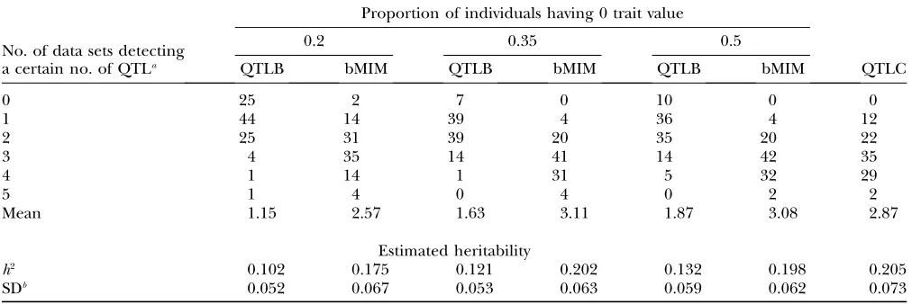
Effects of proportions of categories are studied for binary cases with 20, 30, and 50% of individuals having phenotypic values of 0 (others having 1). Simulation is

done under 4C4Q with h2_{¼0.3. Numbers of data sets}

detecting various numbers of QTL, mean numbers of

detected QTL, and estimatedh2_{(with its standard}

devi-ation) are shown in Table 3. Mapping results are also obtained for the same data sets using QTLB. For mod-erately unevenly divided data (such as a data set with 20% of individuals having a trait value of zero), the majority of data sets detect 2 or 3 QTL (totally 66%). For data sets divided more evenly, more data sets detect 2, 3, or 4 QTL

(.90%). The mean number of detected QTL has

in-creased from 2.57 for data with 20% zeros to3 for cases

with more evenly divided categories. The differences may be partially because with varying proportions of categories, the chances for individuals with various genotypes being in the same category are also changed.

TABLE 2

Critical values for the likelihood-ratio test statistic at significance levels of 0.01 and 0.05

0.01 0.05

h2 _{Method 1/2}a _{4/5 8/9 1/2 4/5 8/9}

0.1 SM 5.71 — — 3.96 — —

RB 5.10 — — 3.89 — —

0.3 SM 5.76 7.32 6.87 3.86 5.23 5.13 RB 5.45 9.26 9.41 3.92 5.63 6.56 0.5 SM 11.00 8.69 6.52 8.07 6.53 4.23 RB 6.72 9.60 8.27 4.50 6.20 6.88 0.8 SM — 13.85 15.26 — 8.41 10.19 RB — 8.90 9.01 — 6.52 6.64

As in the text, direct data simulation and residual bootstrap-ping are abbreviated as SM and RB, respectively. For SM, 1000 different data sets are simulated, and for RB, 1000 data sets are generated by residual bootstrapping from one simulated data set.

a_{Tests are labeled as}

Effects of heritability can be seen in several tables,

such as Tables 4–7. As expected, whenh2_{is higher, all}

methods obtain better mapping results given other situ-ations being the same.

Suitability of using QTL Cartographer/MIM on or-dinal data directly: When the number of categories for an ordinal trait is relatively large, the data can be analyzed by approaches implemented for continuous traits, such as in Visscheret al.(1996), binary traits are analyzed directly by using a linear regression method

proposed by Haley and Knott(1992). However, the

use of Haley–Knott approximation can yield a

sub-stantially inflated residual variance (Xu1995) and

po-tentially decrease the power of detecting QTL. Here we use the maximum-likelihood-based method (MIM mod-ule in QTL Cartographer) to analyze binary/ordinal traits directly, with the hope of remedying part of the inflation.

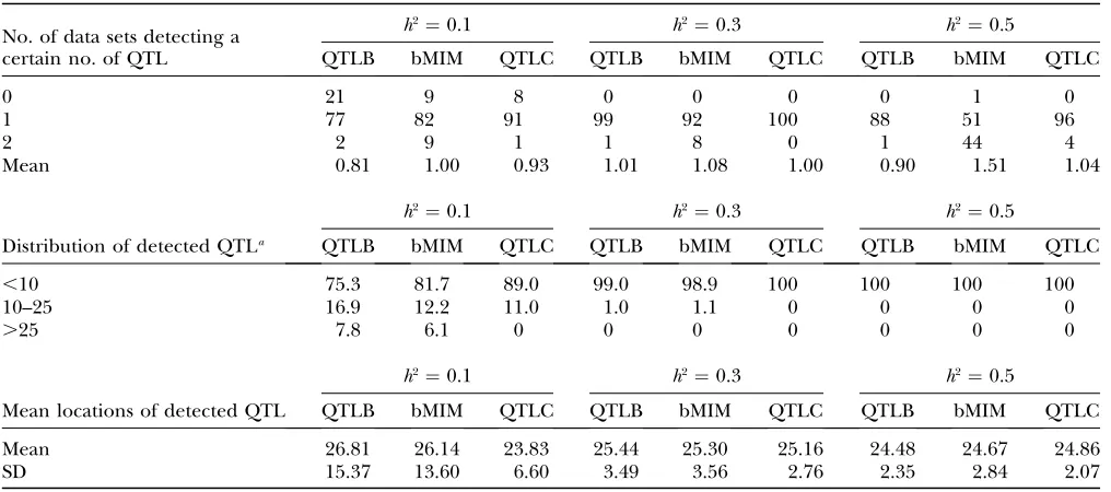
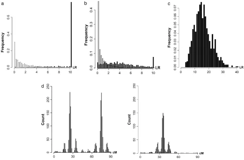
Simulations are performed for different combina-tions of QTL and chromosomes (1C1Q , 2C2Q , 4C4Q , and 8C8Q) with various values of heritability (0.1, 0.3, 0.5, and 0.8). The results are shown in Tables 4–7, with likelihood-ratio profiles from different approaches for 8C8Q shown in Figure 1. By comparing results between QTLB and QTLC and between QTLB and bMIM, we investigated whether/when QTLB can be used. Relative to QTLC, the efficiency of detecting QTL by QTLB

increases with higherh2_{and a lower number of QTL:}

from 60% for 4C4Q (8C8Q) with h2 _{¼ 0.3, under} which the mean number of detected QTL is 1.87 (1.82) for QTLB and 2.87 (2.77) for QTLC, to almost 100% for

1C1Q withh2_{¼0.3. Compared to bMIM, QTLB yields}

similar results whenh2_{is high and the number of QTL is}

low, but has a lower efficiency for lowh2_{or lowh}2_{with a}

high number of QTL. For example, for 2C2Q withh2_¼

0.1, 30% of data sets detect two QTL when bMIM is

applied and only10% when QTLB is used. Generally

speaking, QTLB yield reasonable mapping results when

h2_{is high (say.0.4) and the number of QTL is low (say}

,4).

Loss of information: Binary/ordinal data carry less information than continuous data due to at least two factors. One is that phenotypic values cannot be ranked in detail for ordinal data with only several categories. This lowers the resolution of QTL mapping and reduces the ability of finding QTL with small effects. The other is related to the shape of the distribution of phenotypic values. For ordinal data, trait values concentrate on several separate points instead of covering a region for a continuous trait. This may limit the ability to evaluate mapping results in terms of power and error rate. Since some traits may yield binary/ordinal data only for tech-nical and practical reasons, investigating the efficiency of mapping QTL using binary/ordinal data relative to using continuous data can help us to better understand the limitation of analyzing QTL in experiments pro-ducing binary/ordinal data.

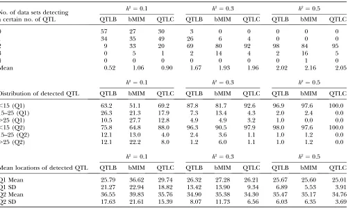
Comparing results from bMIM and QTLC in Tables 4–7, we find that the efficiency of bMIM increases with

higherh2_{. For example, for 2C2Q withh}2_{¼0.1, 51 and}

65% of position estimates by bMIM fall within 15 cM of the two corresponding simulated QTL, respectively,

relative to 69 and 88% by QTLC; whenh2_{increases to}

0.5, the results are 98% and 98% for bMIM and 100% and 100% for QTLC. However, the estimates for QTL

numbers are relatively closer: forh2_{¼0.1, 0.3, and 0.5,}

the numbers are 1.06, 1.93, and 2.16 for bMIM, com-pared to 0.90, 1.96, and 2.05 for QTL, respectively. A

TABLE 3

Estimation results for data with different category proportions

No. of data sets detecting a certain no. of QTLa

Proportion of individuals having 0 trait value

0.2 0.35 0.5

QTLB bMIM QTLB bMIM QTLB bMIM QTLC

0 25 2 7 0 10 0 0

1 44 14 39 4 36 4 12

2 25 31 39 20 35 20 22

3 4 35 14 41 14 42 35

4 1 14 1 31 5 32 29

5 1 4 0 4 0 2 2

Mean 1.15 2.57 1.63 3.11 1.87 3.08 2.87

Estimated heritability

h2 _{0.102 0.175 0.121 0.202 0.132 0.198 0.205}

SDb _{0.052 0.067 0.053 0.063 0.059 0.062 0.073}

Results in this and all following tables are based on 100 simulated data sets, unless indicated otherwise. 4C4Q withh2_{¼0.3 is}

simulated for this table.

a_{Values are the numbers of data sets (of 100) detecting certain numbers of QTL (given in the leftmost column). Mean is}

com-puted asPðNdQNdDÞ=100, whereNdQis the number of detected QTL andNdDis the number of data sets detectingNdQQTL.

similar trend is also seen in multiple QTL and multiple chromosomes cases.

Epistasis: To study epistasis, we adapt an approach using a stepwise model selection scheme in MIM, as

described in Kao_{et al.}(1999) and Zeng_{et al.}(1999). In

this scheme, two types of epistasis can be searched. The first type is the interaction between QTL with main effects. The second one is between QTL with main effects and QTL without main effects. For either type of interaction, epistatic effects are tested for statistical sig-nificance and are added to or dropped from the model on the basis of the testing results. Two case studies are used to illustrate and test our implementation. Details of parameter values are listed in Table 8. Briefly, for all cases three QTL are simulated on two chromosomes at the following positions: 25 cM (QTL 1) and 75 cM (QTL 2) on chromosome 1 and 35 cM (QTL 3) on chromo-some 2. The interaction is between QTL pair 1–3 for all cases. For case 1, all QTL have main effects withVi/Va¼

0.1 (case I-1) or 0.3 (case I-2), whereViandVaare the

epistatic and additive variances, respectively. For case 2 (case II), QTL 1 and 2 have main effects, QTL 3 does not (hence QTL 3 enters into the model only through interaction), andVi/Va¼0.3.

Results are shown in Figure 2, based on 1000 simu-lated data sets with 300 individuals for each set of pa-rameter values. Test statistics of the interaction among different QTL pairs are shown in Figure 2, a (for case I-1) and b (for case I-2). QTL pair with real interaction (QTL

pair 1–3) is detected with a higher probability than other QTL pairs (QTL pairs 1–2 and 2–3). Indeed for 98% of case I-1 and for 88% of case I-2, QTL pair 1–3 has the largest statistic. In Figure 2c, the distribution of the case II test statistic, which is for interaction between detected QTL and regions without detected QTL, is shown. The

distribution has a mean of15 and a variance of37.

About 97% of the test statistics are significant when chi-square distribution is used as an approximation under the null hypothesis. In addition, 97% of these signifi-cant statistics have their corresponding QTL being in accordance with simulated data. Therefore, 94% of tests recover the simulated interaction and consequently, the average number of QTL detected changes from 2.08

when no epistasis is considered to3.02 when epistasis

is considered. The counts of detected QTL based on their estimated locations are shown in Figure 2d.

Limit:It is also interesting to study parameters such as the minimal effect of QTL or maximal number of QTL that can be detected. This is useful in determining the applicability of a method and the validity of its results. Computer simulations are again used for the investiga-tion. A preliminary result for a range ofh2_{-values and the} number of QTL are shown in Table 9. It can be seen that

the mean number of detected QTL increases when h2

increases. For example, for bMIM, the number in-creases from 0.17 to 0.61 for 1C1Q and from 0.18 to

0.37 for 2C2Q, respectively, when h2 _{changes from}

0.01 to 0.05. This is partially expected because QTL

TABLE 4

Estimation results under one-chromosome one-QTL (1C1Q) simulation

No. of data sets detecting a certain no. of QTL

h2_{¼0.1 h}2_{¼0.3 h}2_¼0.5

QTLB bMIM QTLC QTLB bMIM QTLC QTLB bMIM QTLC

0 21 9 8 0 0 0 0 1 0

1 77 82 91 99 92 100 88 51 96

2 2 9 1 1 8 0 1 44 4

Mean 0.81 1.00 0.93 1.01 1.08 1.00 0.90 1.51 1.04

Distribution of detected QTLa

h2_{¼0.1 h}2_{¼0.3 h}2_¼0.5

QTLB bMIM QTLC QTLB bMIM QTLC QTLB bMIM QTLC

,10 75.3 81.7 89.0 99.0 98.9 100 100 100 100

10–25 16.9 12.2 11.0 1.0 1.1 0 0 0 0

.25 7.8 6.1 0 0 0 0 0 0 0

Mean locations of detected QTL

h2_{¼0.1 h}2_{¼0.3 h}2_¼0.5

QTLB bMIM QTLC QTLB bMIM QTLC QTLB bMIM QTLC

Mean 26.81 26.14 23.83 25.44 25.30 25.16 24.48 24.67 24.86

SD 15.37 13.60 6.60 3.49 3.56 2.76 2.35 2.84 2.07

The simulated QTL is located at 25 cM.

a

effects are smaller whenh2_{is smaller and the number of} QTL stays the same. However, no trend for the mean number of the detected QTL is seen when the same

value ofh2_{and different numbers of simulated QTL are}

considered: the results fluctuate from 0.61 to 0.37 to

0.63 for 1C1Q, 2C2Q, and 4C4Q withh2_{¼0.05, when}

bMIM is used. Another useful measurement is the percentage of detected QTL to simulated QTL (or the

ratio between the mean number of detected QTL and

the number of simulated QTL). For 1C1Q with h2 _¼

0.03, 30% of QTL could be detected by all three

approaches; for four QTL withh2_{¼0.1, percentages are}

,30. Note that the numbers are higher for bMIM

for 4C4Q and 8C8Q. This may be due to lower critical values used in bMIM than they should be. Generally

speaking, we expect that when QTL effects are,0.10,

TABLE 5

Estimation results under two-chromosome two-QTL (2C2Q) simulation

No. of data sets detecting a certain no. of QTL

h2_{¼0.1 h}2_{¼0.3 h}2_¼0.5

QTLB bMIM QTLC QTLB bMIM QTLC QTLB bMIM QTLC

0 57 27 30 3 0 0 0 0 0

1 34 35 49 26 6 4 0 0 0

2 9 33 20 69 80 92 98 84 95

3 0 5 1 2 14 4 2 16 5

4 0 0 0 0 0 0 0 1 0

Mean 0.52 1.06 0.90 1.67 1.93 1.96 2.02 2.16 2.05

Distribution of detected QTL

h2_{¼0.1 h}2_{¼0.3 h}2_¼0.5

QTLB bMIM QTLC QTLB bMIM QTLC QTLB bMIM QTLC

,15 (Q1) 63.2 51.1 69.2 87.8 81.7 92.6 96.9 97.6 100.0

15–25 (Q1) 26.3 21.3 17.9 7.3 13.4 4.3 2.0 2.4 0.0

.25 (Q1) 10.5 27.7 12.8 4.9 4.9 3.2 1.0 0.0 0.0

,15 (Q2) 75.8 64.8 88.0 96.3 90.5 97.9 98.0 97.6 100.0

15–25 (Q2) 12.1 13.0 4.0 2.4 3.6 1.1 1.0 1.2 0.0

.25 (Q2) 12.1 22.2 8.0 1.2 6.0 1.1 1.0 1.2 0.0

Mean locations of detected QTL

h2_{¼0.1 h}2_{¼0.3 h}2_¼0.5

QTLB bMIM QTLC QTLB bMIM QTLC QTLB bMIM QTLC

Q1 Mean 25.79 36.62 29.74 26.32 27.28 26.21 25.67 25.60 25.01

Q1 SD 21.27 22.94 18.82 13.42 13.90 9.34 6.89 5.53 3.91

Q2 Mean 36.55 39.83 35.76 34.90 35.38 34.30 35.47 35.17 34.76

Q2 SD 17.63 21.61 15.39 8.07 11.73 6.56 6.03 6.35 3.69

The two simulated QTL are located at 25 cM on chromosome 1 (Q1) and 35 cM on chromosome 2 (Q2), respectively.

TABLE 6

Estimation results under four-chromosome four-QTL (4C4Q) simulation

No. of data sets detecting a certain no. of QTL

h2_{¼0.3 h}2_{¼0.5 h}2_¼0.8

QTLB bMIM QTLC QTLB bMIM QTLC QTLB bMIM QTLC

0 10 0 0 0 0 0 0 0 0

1 36 4 12 2 0 0 0 0 0

2 35 20 22 13 1 0 0 0 0

3 14 42 35 37 14 5 0 0 0

4 5 32 29 46 61 87 93 58 78

5 0 2 2 2 20 8 6 28 21

6 0 0 0 0 4 0 1 14 1

Mean 1.87 3.08 2.87 3.33 4.12 4.03 4.08 4.56 4.23

the percentage of detected QTL will be around or

,5%, which is close to the rate of random errors and

therefore may be close to QTL detection limits for these methods.

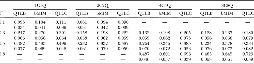
Approximation ofh2_:R2_{of the fitted models can be}

used to approximateh2_{, such as in QTLC and QTLB.}

For ordinal data using bMIM, the estimate ofh2_{can be}

approximated by an alternative form ofR2_{designed for}

logistic regression, suggested by Nagelkerke(1991),

R_L;2_adj¼R_L2=R_L;2_max;

which is an adjusted form ofRL2 proposed by Maddala

(1983), Coxand Snell(1989), and Magee(1990),

R_L2¼1 ðL0=L1Þ2=N;

where L0 is the likelihood under the null model (no

QTL),L1is the maximum likelihood under the

alter-native model (a certain number of QTL exist), andNis

the sample size.RL2,maxis the maximal possible value for

RL2 and is equal to 1 L02/N. Note that RL2,adj ranges

between 0 and 1.

Using the simulated data sets of Tables 4–7, results of

approximating h2 _{are summarized in Table 10. These}

results suggest that better approximation of h2 _is

ob-tained when underlying heritability (denoted by hR2)

increases for a specific combination of numbers of QTL

and chromosomes and that for the same hR2 value, a

smaller number of QTL generally result in a better approximation ofh2_{. For example, forh}

R

2_{¼0.3, estimates}

ofh2_{are 0.247, 0.270, and 0.301 by QTLB, bMIM, and}

QTLC, respectively, for 1C1Q, and 0.132, 0.198, and 0.205, respectively, for 4C4Q. These results are somehow expected: with a lower underlying heritability and/or greater number of QTL, QTL effects are smaller, and this will make it more difficult to detect these QTL. The model then will explain a smaller amount of total

variation. In addition, QTLC has the best estimates and bMIM yields better results than QTLB does, especially for large number of QTL/chromosome situations.

IMPLEMENTATION IN QTL CARTOGRAPHER

We have implemented the procedures of categorical trait MIM (CT–MIM) in version 2.5 of Windows QTL

Cartographer (Wanget al. 2005). Categorical traits are

coded in integer value and can be input into the program in the same way as continuous traits. One can use the categorical trait analysis to perform interval mapping (CT–IM) and multiple-interval mapping (CT– MIM) analysis. One can also use the regular IM, CIM, and MIM, implemented for continuous traits, to analyze the data for comparison.

For model selection in CT–MIM, we implemented several interactive procedures. They include a proce-dure that selects an initial model on the basis of forward or backward stepwise logistic regression on markers, a procedure to search for more QTL one at a time, a procedure to search for epistasis of QTL, a procedure to test effects of selected QTL, a procedure to optimize positions of QTL, and a procedure to output the complete information of the selected model. These procedures can be used interactively in practical data analysis to explore the data and compare different models. For more information see the software manual (http://statgen.ncsu.edu/qtlcart/WQTLCart.htm).

DISCUSSION

Kao et al. (1999) developed MIM for QTL analysis that fits a multiple-QTL model and simultaneously searches for the positions and interaction patterns of multiple QTL. This multiple-QTL-oriented approach has a number of advantages, such as improved statistical

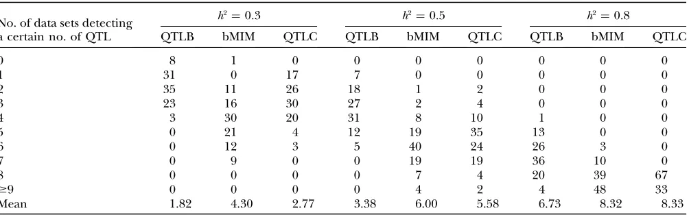
TABLE 7

Estimation results under eight-chromosome eight-QTL (8C8Q) simulation

No. of data sets detecting a certain no. of QTL

h2_{¼0.3 h}2_{¼0.5 h}2_¼0.8

QTLB bMIM QTLC QTLB bMIM QTLC QTLB bMIM QTLC

0 8 1 0 0 0 0 0 0 0

1 31 0 17 7 0 0 0 0 0

2 35 11 26 18 1 2 0 0 0

3 23 16 30 27 2 4 0 0 0

4 3 30 20 31 8 10 1 0 0

5 0 21 4 12 19 35 13 0 0

6 0 12 3 5 40 24 26 3 0

7 0 9 0 0 19 19 36 10 0

8 0 0 0 0 7 4 20 39 67

$9 0 0 0 0 4 2 4 48 33

Mean 1.82 4.30 2.77 3.38 6.00 5.58 6.73 8.32 8.33

power in QTL detection, facilitation for analyzing QTL epistasis, and coherent estimation of overall QTL param-eters. The implementation of the MIM method in QTL

Cartographer (Basten et al. 2005) and Windows QTL

Cartographer (Wanget al. 2005), both freely available at

http://statgen.ncsu.edu/qtlcart/, has greatly facilitated applications of the method for general QTL mapping

data analysis. However, the MIM method of Kao et al.

(1999) and its implementation in QTL Cartographer and Windows QTL Cartographer is for continuous traits.

Although extensive research has been made that takes multiple QTL into account in mapping analysis on

binary and ordinal traits (e.g., Yi and Xu 2000; Yi

et al. 2004), no computer program is available for QTL mapping data analysis on ordinal traits under the MIM framework.

In this study, we extend MIM to ordinal traits on the basis of a threshold model. This extension utilizes the properties and advantages of MIM for QTL mapping analysis on ordinal traits. The method fits a model of

multiple-QTL effects and epistasis on the underlying liability and searches for the number and positions of QTL and epistasis simultaneously. It has similar advan-tages to MIM on the statistical power of QTL detection

and estimation of overall QTL parameters. The imple-mentation of this method in Windows QTL Cartogra-pher will greatly facilitate the general usage of the methodology for QTL mapping data analysis on binary and ordinal traits.

Using simulations, we investigated several statistical issues, such as the effect of trait distribution on QTL mapping results, comparison of QTL mapping on an ordinal trait and on a continuous trait, and the statistical power of the method for QTL detection. As expected, the larger the number of trait categories, the higher the statistical power for QTL detection. There is not much difference in mapping results to regard an ordinal trait with five or more categories as a continuous trait in QTL analysis (data not shown). Also it is interesting to ob-serve that if we regard a binary trait as a continuous trait using the current MIM in QTL Cartographer, the map-ping result is actually quite comparable to that using the threshold MIM model if the heritability is reasonably high. Of course, the threshold MIM model is always more powerful and appropriate for QTL mapping analysis on binary and ordinal traits.

TABLE 8

List of epistatic situations

QTL no.

Chr no.

Position (cM)

Main

effect Epistasis

Epistatic effect

I-1 1 1 25 0.845 1 and 3 2.31

2 1 75 0.845

3 2 35 0.845

I-2 1 1 25 0.987 1 and 3 1.21

2 1 75 0.987

3 2 35 0.987

II 1 1 25 1.061 1 and 3 1.92

2 1 75 1.061

3 2 35 0.000

h2_{¼0.5 for all cases, and 1000 data sets of 300 individuals}

are simulated for each case.

Figure2.—Results for cases with epistatic effects. (a) Distribution of test statistic for case I-1: main effects for all QTL and the epistatic effect for QTL pair 1–3 withVi/Va¼0.3. (a and b) Solid bars represent the test statistic (LR) for QTL pair 1–3 and open

bars the LR for other pairs (QTL pairs 1–2 and 2–3). (b) Distribution of the test statistic for case I-2, which is the same as case I-1 exceptVi/Va¼0.1. Note that in a and b, the rightmost bars represent test statistics$10. (c) Distribution of the test statistic for case

In studying ordinal traits, the trait value of an in-dividual may be misspecified due to measurement error.

For a binary trait, Rousseeuwand Christmann(2003)

used a ‘‘hidden logistic regression model’’ with the assumption that an observed response has a small chance to be measured with error. This can occur when a binary or ordinal phenotype is difficult to classify. A model with measurement error similar to that of Rousseeuwand Christmann(2003) can also be used for our analysis. This can be done by reassigning the value ofPðzijyi;GÞ in Equation 4. Namely, instead of being either 1 or 0, it can be 1eiandei, whereeiis a small nonnegative value for error rate. This error rate can be assumed to be the same for all observations or different for different observations.

In this article, we used the maximum-likelihood ap-proach for mapping multiple QTL on binary and ordinal traits. The Bayesian approach has also been used extensively for QTL mapping analysis in designed

experiments, such as in Thomasand Cortessis(1992),

HoescheleandvanRaden(1993a,b), Satagopanand Yandell (1996), and Sillanpa¨ a¨ and Arjas (1998, 1999). For binary and ordinal traits, a series of studies

have been performed by Xu and Atchley (1996), Yi

and Xu(1999a,b, 2000), and Yiet al.(2004) to develop

statistical methods for mapping multiple QTL under a

Bayesian framework combined with Markov chain Monte Carlo sampling with a reversible-jump algorithm for model selection. These methods, based on a threshold model for binary/ordinal traits, are comparable to our maximum-likelihood method. However, despite the ex-tensive studies performed, no user-friendly software is publicly available for QTL mapping data analysis on binary/ordinal traits. The statistical methods described in this article will be implemented in QTL Cartographer and Windows QTL Cartographer and publicly distributed at http://statgen.ncsu.edu/qtlcart/ for general usage of mapping multiple QTL on binary and ordinal traits.

There are still some issues that deserve further in-vestigation. Currently, we use a procedure suggested by

Linand Zou(2004) to estimate the threshold at each

step of searching for new QTL to aid in model selection. This procedure performs a function similar to a per-mutation test, but is numerically much more efficient. However, it is still not quite clear yet what significance level one needs to use in this stepwise procedure in the context of model selection for multiple QTL with epistasis. We will further pursue this line of research.

We thank Yongqiang Tang for help in computer programming. This work was partially supported by National Institutes of Health grant GM45344 and U.S. Department of Agriculture Plant Genome grant 2003-00754.

TABLE 9

Limits of different approaches

1C1Q 2C2Q 4C4Q 8C8Q

h2_{: 0.01 0.03 0.05 0.01 0.03 0.05 0.05 0.10 0.20 0.05 0.10 0.20}

Effect: 0.20 0.35 0.46 0.11 0.19 0.25 0.18 0.26 0.38 0.12 0.18 0.27

The mean no. of detected QTL

QTLB 0.10 0.23 0.42 0.04 0.14 0.17 0.29 0.46 0.73 0.24 0.37 0.90 bMIM 0.17 0.39 0.61 0.18 0.29 0.37 0.63 1.02 1.98 1.47 2.24 3.41 QTLC 0.11 0.34 0.64 0.06 0.16 0.33 0.37 0.78 1.64 0.43 0.78 1.62

TABLE 10

Estimate of heritability for ordinal data

1C1Q 2C2Q 4C4Q 8C8Q

h2 _{QTLB bMIM QTLC QTLB bMIM QTLC QTLB bMIM QTLC QTLB bMIM QTLC}

0.1 0.093 0.104 0.111 0.081 0.094 0.090 — — — — — —

0.034 0.041 0.039 0.031 0.042 0.039 — — — — — —

0.3 0.247 0.270 0.301 0.158 0.198 0.222 0.132 0.198 0.205 0.128 0.237 0.180 0.066 0.056 0.054 0.058 0.062 0.059 0.059 0.062 0.073 0.056 0.068 0.079 0.5 0.482 0.483 0.499 0.282 0.332 0.387 0.264 0.346 0.385 0.234 0.378 0.384 0.077 0.069 0.048 0.061 0.070 0.059 0.070 0.072 0.053 0.076 0.073 0.082

0.8 — — — — — — 0.487 0.601 0.696 0.483 0.645 0.723

— — — — — — 0.046 0.057 0.039 0.058 0.061 0.039

For each value forh2_{, its estimates from different approaches are listed in the top row with standard deviation given in the}

LITERATURE CITED

Basten_{, C., B. S. W}eir_{and Z-B. Z}eng_{, 2005 QTL Cartographer.}

Department of Statistics, North Carolina State University, Raleigh, NC (http://statgen.ncsu.edu/qtlcart/).

Broman, K. W., 2003 Mapping quantitative trait loci in the case of a

spike in the phenotype distribution. Genetics163:1169–1175. Broman, K. W., and T. P. Speed, 2002 A model selection approach

for the identification of quantitative trait loci in experimental crosses. J. R. Stat. Soc. Ser. B64:641–656.

Cox, D., and E. Snell, 1989 _{The Analysis of Binary Data}, Ed. 2.

Chapman & Hall, London.

Dempster, A. P., N. M. Lairdand D. B. Rubin, 1977 Maximum

like-lihood from incomplete data via the EM algorithm. J. R. Stat. Soc. Ser. B39:1–38.

Falconer_{, D. S., 1965 The inheritance of liability to certain diseases,}

estimated from the incidence among relatives. Ann. Hum. Genet. 29:51–71.

Falconer, D. S., and T. F. C. Mackay, 1996 Introduction to Quantita-tive Genetics, Ed. 4. Addison–Wesley, Boston.

Fisher_{, R. A., 1918 The correlation between relatives on the}

supposi-tion of Mendelian inheritance. Trans. R. Soc. Edinb.52:399–433. Hackett_{, C. A., and J. I. W}eller_{, 1995 Genetic mapping of}

quan-titative trait loci for traits with ordinal distributions. Biometrics 51:1252–1263.

Haley, C. S., and S. A. Knott, 1992 A simple regression method for

mapping quantitative trait loci in line crosses using flanking markers. Heredity69:315–324.

Hoeschele, I., and P.vanRaden, 1993a Bayesian analysis of

link-age between genetic markers and quantitative trait loci. I. Prior knowledge. Theor. Appl. Genet.85:953–960.

Hoeschele_{, I., and P.}van_Raden_{, 1993b Bayesian analysis of}

link-age between genetic markers and quantitative trait loci. II. Com-bining prior knowledge with experimental evidence. Theor. Appl. Genet.85:946–952.

Jansen_{, R. C., 1993 Interval mapping of multiple quantitative trait}

loci. Genetics135:205–211.

Jiang_{, C., and Z-B. Z}eng_{, 1997 Mapping quantitative trait loci with}

dominant and missing markers in various crosses from two in-bred lines. Genetica101:47–58.

Kao_{, C.-H., and Z-B. Z}eng_{, 1997 General formulas for obtaining the}

MLEs and the asymptotic variance-covariance matrix in mapping quantitative trait loci when using the EM algorithm. Biometrics 53:653–665.

Kao_{, C.-H., Z-B. Z}eng_{and R. D. T}easdale_{, 1999 Multiple interval}

mapping for quantitative trait loci. Genetics152:1203–1216. Lander_{, E. S., and B. B}otstein_{, 1989 Mapping Mendelian factors}

underlying quantitative traits using RFLP linkage maps. Genetics 121:185–199.

Lin, D., and F. Zou, 2004 Assessing genomewide statistical

signifi-cance in linkage studies. Genet. Epidemiol.27:202–214. Maddala_{, G. S., 1983 Limited-Dependent and Qualitative Variables in}

Econometrics.Cambridge University Press, Cambridge, UK. Magee_{, L., 1990 R}2_{measures based on Wald and likelihood ratio}

joint significance tests. Am. Stat.44:250–253.

Nagelkerke_{, N., 1991 A note on the general definition of the}

co-efficient of determination. Biometrika78:691–692.

Rousseeuw, P. J., and A. Christmann, 2003 Robustness against

separation and outliers in logistic regression. Comp. Stat. Data Anal.43:315–332.

SAS Institute_{, 1999 SAS/STAT User’s Guide, Version 8. SAS Publishing,}

Cary, NC.

Satagopan_{, J. M., and B. S. Y}andell_{, 1996 Estimating the number}

of quantitative trait loci via Bayesian model determination. Joint Statistical Conference, Chicago (ftp://ftp.stat.wisc.edu/pub/ yandell/revjump.ps.gz).

Sillanpa¨ a¨, M. J., and E. Arjas, 1998 Bayesian mapping of multiple

quantitative trait loci from incomplete inbred line cross data. Genetics148:1373–1388.

Sillanpa¨ a¨_{, M. J., and E. A}rjas_{, 1999 Bayesian mapping of multiple}

quantitative trait loci from incomplete outbred offspring data. Genetics151:1605–1619.

Thomas, D. C., and V. Cortessis, 1992 A Gibbs sampling approach

to linkage analysis. Hum. Hered.42:63–76.

Visscher, P. M., C. S. Haleyand S. A. Knott, 1996 Mapping QTLs

for binary traits in backcross and F2populations. Genet. Res.68: 55–63.

Wang, S., C. J. Bastenand Z-B. Zeng, 2005 _{Windows QTL} Cartogra-pher 2.5.Department of Statistics, North Carolina State Univer-sity, Raleigh, NC (http://statgen.ncsu.edu/qtlcart/WQTLCart. htm).

Wright, S., 1934a An analysis of variability in number of digits in an

inbred strain of guinea pigs. Genetics19:506–536.

Wright, S., 1934b The results of crosses between inbred strains of

guinea pigs, differing in number of digits. Genetics19:537–551. Xu_{, S., 1995 A comment on the simple regression method for}

inter-val mapping. Genetics141:1657–1659.

Xu_{, S., and W. R. A}tchley_{, 1996 Mapping quantitative trait loci for}

complex binary diseases using line crosses. Genetics143:1417– 1424.

Yi, N., and S. Xu, 1999a Mapping quantitative trait loci for complex

binary traits in outbred populations. Heredity82:668–676. Yi, N., and S. Xu, 1999b A random model approach to mapping

quantitative trait loci for complex binary traits in outbred popu-lations. Genetics153:1029–1040.

Yi, N., and S. Xu, 2000 Bayesian mapping of quantitative trait loci

for complex binary traits. Genetics155:1391–1403.

Yi, N., and S. Xu, 2002 Mapping quantitative trait loci with epistatic

effects. Genet. Res.79:185–198.

Yi, N., S. Xu, V. Georgeand D. B. Allison, 2004 Mapping multiple

quantitative trait loci for ordinal trait. Behav. Genet.34:3–15. Zeng, Z-B., 1993 Theoretical basis for separation of multiple linked

gene effects in mapping quantitative trait loci. Proc. Natl. Acad. Sci. USA90:10972–10976.

Zeng, Z-B., 1994 Precision mapping of quantitative trait loci. Genetics

136:1457–1468.

Zeng, Z-B., C.-H. Kaoand C. J. Basten, 1999 Estimating the genetics

architecture of quantitative traits. Genet. Res.74:279–289. Zeng, Z-B., J. Liu, L. F. Stam, C.-H. Kao, J. M. Marcer et al.,

2000 Genetic architecture of a morphological shape difference between two Drosophila species. Genetics154:299–310.

Communicating editor: M. S. McPeek

APPENDIX A: THEQ-FUNCTION AND ITS DERIVATIVES

TheQ-function is defined as the expectation of log-likelihood function for the complete data (Dempsteret al. 1977). In our study, QTL genotypes are unknown and have to be inferred from marker genotypes. This can be dealt

with by theQ-function and the process is briefly described below as

QðBjBðtÞ_{Þ ¼}

E_BðtÞ½logL_cðfZ;Qg_complete;BÞ j fZ;Mg_obs;

whereB¼ ðGT_;QT_;DT_ÞT

is the vector of parameters to be estimated, and the superscripttindicates thetth cycle of the

iteration. Since the realBis unknown, we compute theQ-function on the basis of its value at thetth stage. This is

symbolized asQðBjBðtÞ_{Þ. The subscript for the expectation sign}

Eindicates that the expectation is computed using a

observed data {Z,M}obs. Using definitions of expectation and conditional probability and assuming independent

sampling, we have

QðBjBðtÞ_{Þ ¼}

E_BðtÞ½logL_cðfZ;Qg_complete;BÞ j fZ;Mg_obs

¼X

N

i¼1

X

Qih

½P_B¼BðtÞðQ_ihjz_i;M_iÞlogP_B¼BðtÞðz_i;Q_ihÞ

¼X

N

i¼1

X

Qih

fP_B¼BðtÞðQ

ihjzi;MiÞlog½PB¼BðtÞðz_ijQ

ihÞPðQihÞg

¼X

N

i¼1

X

Qih

½P_B¼BðtÞðQ

ihjzi;MiÞlogPB¼BðtÞðz_ijQ

ihÞ1C; ðA1Þ

whereCis the probability of the observed data and is a constant. Therefore,Ccan be omitted where maximization of

theQ-function is concerned. By Bayes’ theorem and noting thatPB¼B(t)(zijQih,Mi)¼PB¼B(t)(zijQih), we have

Lð_ihtÞ¼P_B¼BðtÞðQ_ihjz_i;MiÞ ¼

P_B¼BðtÞðz_ijQ

ih;MiÞPB¼BðtÞðQ ihjMiÞ

P

Qil½PB¼BðtÞðzijQil;MiÞPB¼BðtÞðQiljMiÞ

: ðA2Þ

Here,Lih(t)can be considered as a posterior probability forQih. Equation A1 can then be written as

QðBjBðtÞÞ ¼X N

i¼1

X

Qih

fLð_ihtÞlog½FQ_ihðgzi11Þ FQihðgziÞg: ðA3Þ

With a logistic-distributed liability and denoting B0¼ ðGT;QTÞ

T

, Equation A3 can be written as QðBjBðtÞ_{Þ ¼}

PN

i¼1 P

Qih½

Lð_ihtÞlogðp_zi11;ihpzi;ihÞwith

pk;ih¼pðBT0xk;ihÞ ¼expðtBT0xk;ihÞ=½11expðtBT0xk;ihÞ; ðA4Þ

where subscriptihindicates thehth QTL genotype for theith individual, andB0¼ ðGT;QTÞTis a parameter vector for

the thresholds and QTL effects. In addition,xk,ih¼(lkT,xihT)T, wherelk(k¼0,. . .,n1) is ann31 vector with all

elements being 0 except the (k11)th element being 1. Define

bih ¼pzi11;ihpzi;ih

and

aih ¼@bih=@B0¼pzi11;ihð1pzi11;ihÞxzi11;ihpzi;ihð1pzi;ihÞxzi11;ih:

Noting that@pk,ih/@B0¼pk,ih(1pk,ih)xk,ih, we have

@QðBjBðtÞÞ

@B0

¼X

N

i¼1

X

Qih

Lð_ihtÞ@logðpzi11;ihpzi;ihÞ

@B0

¼X N i¼1 X Qih

Lð_ihtÞ p_zi11;ihpzi;ih

@p_zi11;ih

@B0

@pzi;ih

@B0

¼X N i¼1 X Qih

Lð_ihtÞaih bih

:

ðA5Þ

Further differentiating the first derivative, we have the second derivative as

@2QðB0jBð₀tÞÞ

@B0@BT₀ ¼

XN

i¼1

X

Qih

Lð_ihtÞ

b_ih2 3

@ðaih=bihÞ

@BT₀ ¼

XN

i¼1

X

Qih

Lð_ihtÞ

b_ih2 bih

@aih

@BT₀ aih

@bih

@BT₀

¼X N i¼1 X Qih

Lð_ihtÞAihbihaiha T

ih

b_ih2 ; ðA6Þ

where

Aih¼

@aih

@BT₀ ¼

@2_b

ih

@B0@BT0

¼pzi11;ihð1pzi11;ihÞð12pzi11;ihÞxzi11;ihx

T

zi11;ihpzi;ihð1pzi;ihÞð12pzi;ihÞxzi;ihx

T

APPENDIX B: THE ITERATIVE PROCESS FOR THE NR–EM ALGORITHM

For a set of fixed QTL positions, an approach combining Newton–Raphson (NR) and EM algorithms can be used to obtain estimates of other parameters such as QTL effects. A brief description of the iterative process is given below:

1. InitializeB0

(0) .

2. UpdateLih

(t)

in Equation A2 (the E-step) andpihin Equation A4.

3. Obtain the first derivative (g(t)_{) and second derivative (H}(t)_{) using Equations A5 and A6.}

4. UpdateB0

(t11)

using a formula

Bð₀t11Þ¼Bð₀tÞb½HðtÞ1_gðtÞ_;

where the superscript ‘‘1’’ indicates the inverse of a matrix, and the inverse ofHcould be obtained by Cholesky

decomposition. Several EM steps may be performed in the case that the decomposition fails.

5. Find the new value of theQ-function atB0

(t11)

by Equation A3.

6. Determine whether the iteration process converges, usually by comparing the relative change of the Q to a

convergence tolerance (d). If the change of theQ-function is smaller thand, stop; if not, go back to step 2.

Note that two parameters (bandd) in the above process need to be preset.bis a scalar and characterizes the step

length in the gradient direction. It should not be too large (missing maximum) or too small (slow convergence).

During computation,bwill start at one and reduce its value gradually in each cycle if needed, but it will be reset to one

in a new iteration cycle. The value ofdcan be determined through several methods. Here, we take the simplest one: set