R E S E A R C H
Open Access
Column generation for frequency assignment
in slow frequency hopping networks
Arie Koster and Martin Tieves
*Abstract
This article deals with the frequency assignment problem (FAP) in slow frequency hopping (GSM) networks, a generalization of the classical FAP. Due to symmetry in the solutions, a natural integer linear programming
formulation does not yield a good solution procedure. Instead, we decompose the co-channel and adjacent channel interference minimization and develop a two-stage algorithm. The co-channel optimization problem is solved with a column generation model, whereas the second stage is solved by a cutting plane approach. Computational
experiments reveal, that although no optimal solutions can be guaranteed, the approach provides promising results, both regarding practical applicability and further research potential.
Keywords: Slow frequency hopping, Interference minimization, Column generation
Introduction
Mobile communication, as a key aspect of modern society, looks upon a history of success and growth. Consequen-tially, a wide range of organizational questions, connected to a network’s structure and usage, have been in the focus of research ever since. This article concentrates on fre-quency planning. Mobile communication physically takes place in the radio spectrum. This spectrum is a limited resource, it can only support a finite number of fre-quencies. Consequently, a sensible assignment of these frequencies to signal emitters is necessary. On the back-ground of GSM technology or modified for more modern standards like WLAN, UMTS, and LTE, the settings of the classical frequency assignment problem (FAP) have com-monly been accepted as an insightful point of research for questions related to FAPs. FAP focuses on the optimiza-tion of mobile communicaoptimiza-tion quality by means of min-imizing mutual (co- and adjacent channel) interference between signal transceivers (TRX).
Clearly, the FAP is a highly abstracted model of reality. In this article, the difficulties of obtaining these (interfer-ence) values and other influencing factors of communi-cation quality among power control techniques, adaptive modulation, or channel utilization are not treated in
*Correspondence: [email protected] Lehrstuhl 2 f ¨ur Mathematik, RWTH, Aachen, Germany
detail. However, especially the topics adaptive modula-tion and power-control play important roles in resource management and are closely related to questions of transmission quality since both have a direct impact on interference measures. We refer to [1-3] for in-depth information on adaptive modulation and to [4,5] for infor-mation on power-control techniques. In this article, we focus on the abstract mathematical optimization prob-lem and assume these influences sufficiently clarified beforehand.
While the FAP considers a static assignment of fre-quencies to signal emitters (one channel per TRX), the concept of slow frequency hopping (SFH) is going beyond this one-to-one mapping and assigns multiple frequen-cies to each TRX. In SFH, a TRX does not transmit permanently on one frequency, but changes its trans-mitting frequency within a specific frequency pool at random periods. Hereby, the main goal of FAP persists: minimizing the total expected (mutual) interference of these assignments. The focal point of SFH, randomiza-tion, incorporates statistical effects, leading to interfer-ence and frequency diversity. Basically, this means that frequency-related characteristics are averaged. For exam-ple, signal-spreading is highly frequency related, such that the extreme peeks in signal distribution are cut off by SFH on average. Signals at a specific location are no longer either very bad (unusable) or very good (ineffi-cient) the whole time, though bad conditions on isolated
time frames are still very possible since they can be eas-ily corrected via error recognition codes. Here we refer to [6-8] for more information. Thus, randomization effec-tively lowers the network’s signal-to-noise ratio, resulting in an increased capacity or improved transmission quality compared to non-hopping networks. In the following, this problem is denoted with SFH-FAP.
In this study, the problem of finding frequency assign-ments for SFH networks is formulated by means of mixed integer programming. Hereby, SFH-FAP is interpreted as an advancement of FAP (see [9] for a survey on FAP). Since a column generation approach is invoked here, the work of Jaumard (and others) is to mention, for exam-ple [10-12]. There, a similar problem is analyzed, enriched with the aspects of antenna spacing but reduced to inter-preting interference values not as floating numbers but only as integer levels (interference possible from 0 to 10). Performing column generation as well, their approach is closely related to the graph coloring problem in Mehrotra and Trick [13].
Concerning SFH-FAP, frequency planning has been done on a heuristic basis, mostly. Here one could mention the papers [14-16]. There, frequency assignments are cre-ated by the means of frequency lists for each transceiver, which are created and improved on a heuristic basis (e.g., by simulated annealing). While these methods are usu-ally fast, they cannot claim to provide optimal frequency assignments. In contrast to these approaches, this arti-cle tries to invoke exact methods for obtaining optimal frequency assignments. Therefore, advanced optimization concepts like column generation and cutting plane algo-rithms are used. Though frequency assignments can be provided, no guarantees of optimality can be given. Never-theless, this article analyzes the usage of the chosen means and points out future research potential. On the whole, this study is based on the master thesis of Tieves [17].
In the following, the problem description is formal-ized and a mixed integer formulation is given. Next, the problem is decomposed into two sub-problems, treated consecutively. The resulting optimization procedure is evaluated for modified test examples from the FAP web-site [18]. At the end of this article, some conclusions of this approach as well as future research proposals are given.
Problem description
First, the input of the classical FAP is briefly summarized and the SFH-FAP input is evolved from this. A math-ematical problem description is presented, leading to a mixed integer formulation of this problem at the end of the section.
Frequency assignments in GSM networks
A detailed description of the FAP problem in GSM net-works can be found in [19]. There, the FAP is deeply
explained and information are given, how the model, i.e., the interference values can be derived from reality. Here we focus on the abstracted mathematical optimiza-tion problem and invoke no deepening research on these matters.
From a mathematical perspective, an instance of the FAP can be interpreted as an undirected graphG=(T,E) and a setF of available frequencies. We assume that the frequencies are equally spaced in the radio spectrum. The verticesv ∈ T represent the signal emitters (TRXs). For every edgee= {v1,v2} ∈Ewithv1,v2∈T,co(v1,v2)≥0 and ad(v1,v2) ≥ 0 define the amount of co- and adja-cent channel interference, which is induced if both TRXs transmit on the same, respectively, neighboring frequen-cies. Further a separation distance dv1,v2 ∈ Nmight be
defined for edges {v1,v2} ∈ E, specifying the minimum distance between the transmissions ofv1andv2in the fre-quency spectrum. For every vertexv∈T, a set of (locally)
blocked frequenciesBv ⊂ F might be defined,
contain-ing the frequencies which cannot be assigned to this TRX. The aim is to find a frequency assignment, i.e., a mapping of one frequencyf ∈Fto every TRXv∈T, such that the separation and blocking constraints are met and the total induced co- and adjacent channel interference is minimal. In this context, the interference values can be interpreted as costs or penalties as well.
SFH
For a FAP-SFH instance, as a generalization of the FAP problem, we assume that two additional inputs are com-plementing the FAP input. First, a partition of the TRXs is provided, i.e., a collectionS = {I1,. . .,Ip}withIi ⊆ S,
p
i=1Ii = T andIi∩Ij = ∅for alli = j. For eachithe set of TRXsIiis called super transceiver (STRX) in the
fol-lowing. Second, for everyI ∈ Sa valuekI ∈ Ndenoting
the required amount of frequencies of this STRX is given. As an interpretation: Each TRXvis in one STRXIand at every time frame,vchooses a frequencyf to transmit on, out of thekIavailable ones, at random uniformly and
inde-pendently distributed. Hereby the STRX structure shows, which TRXs may potentially choose the same frequencies. Now an assignment should be provided, which assigns kIfrequencies to every STRXIsuch that the quality is as
averaged quality—the single time-frame cannot be distin-guished by the human ear. Because of the randomization, in every single time-frame the frequency assignment pro-duces a higher interference level compared to a FAP assignment, however the frequency hopping gain sur-passes the higher average interference. Nevertheless, we assume the expected interference as a suitable measure for obtaining frequency assignments. For each pair of STRXsI andJ, these expected co- and adjacent channel interferences co(I,J) and ad(I,J) can be determined as follows.
Given a frequencyf assigned to both STRXIand STRX
J, the probability that two TRXs v ∈ I and w ∈ J
choose this frequency simultaneously is k1
I·kJ, inducing a co-channel interferenceco(v,w). Hence, the expected co-channel interference isco(I,J)·yI,J whereyI,J denotes the
number of equal channels assigned toIandJand
co(I,J):=
Similarly, the expected adjacent channel interference is ad(I,J)·nI,JwherenI,Jis the number of adjacent channels
assigned toIandJand
ad(I,J):=
Summing up the differences between FAP and SFH-FAP, the interference on TRX level is aggregated to the STRX level such that the induced interference between two STRXs is the total (expected) interference of the inbound TRXs. Nevertheless, an SFH-FAP instance is similar to an FAP instance, with the difference, that for the nodes corre-sponding to an STRX more than one frequency per node is needed and the edge-weights are adapted in the above way (1), (2). The downside of this aggregation lies within the separation and blocking constraints. When aggregating the TRXs to the STRX level, separations may be specified between two STRXs (denoted withdI,J ∈ N) or between
each TRX within a STRX (denoted by dI ∈ N).
How-ever, since the frequencies for each TRX in the STRX are drawn at random, no separation can be guaranteed on the inner TRX level any longer. Furthermore, separations on the STRX level hold for all TRXs within these STRXs such that not all constraints can be aggregated and those which are lifted to the STRX level may be more striking than before. Additionally, the same applies for the blocking constraints.
Note that these disadvantage arises from considering arbitrary STRX structures. Establishing a frequency hop-ping structure in a network, it is always possible to regard each single TRX as STRX. Then, all separations/blocking constraints can be transported into that framework. How-ever, the mathematical consequence is a greatly enlarged
problem size. In practical aspects, some trade-off between problem-size and correctness is reasonable. Incorporat-ing SFH at the expense of some inaccuracy within the constraints may still improve the overall network quality.
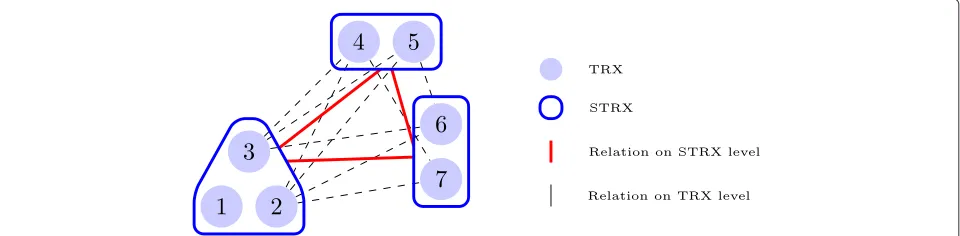
As an example of this transformation, one may consider Figure 1. Given the set of TRXs asT := {1,. . ., 7}, the
set of all STRXs may be formed of three STRXs S :=
{I1,I2,I3}. In this example,I1consists of the TRXs one to three,I2 contains four and five and STRXI3 consists of the remaining TRXs. The relations (co-, adjacent chan-nel interference, separations, and blockings) on TRX level, here shown as dotted, are aggregated to STRX level (red lines) via the procedure mentioned above. The random-ization of SFH is incorporated in the STRX relations, the interference values are expected values and no fixed, mea-surable information any longer. For clearness sake, the interference relations “within” a single STRX have been omitted. Given a STRXI, co(I,I) is a constant for every frequency assigned, determined by the STRX structure, i.e., the inbound TRXs. For the expected co-channel inter-ference, this constant is multiplied with the amount of fre-quencies to be assigned, an other constant (yI,I=kI). As a
result the co-channel interference value within a STRX is already determined by the STRX structure and indepen-dent from the specific frequency assignment. However, inner STRX adjacent channel interference is not a con-stant and can be determined as described in (2).
In summary, SFH-FAP aims to find an optimal fre-quency assignment, i.e., assign at leastkIfrequenciesf ∈
Fto every STRXIsuch that the expected induced inter-ference is minimal, all separation/blocking constraints are met and the totally induced expected co- and adjacent channel interference is minimal. This can be formalized as follows.
The input for the SFH-FAP problem is a nine-tuple M := (S,E,F,{BI}I∈S,kI,dI,dI,J,co,ad). A feasible
solu-tion, i.e., a feasible assignment, is a function
Y :S →2F,
mapping each vertex to a set of frequencies such that
|Y(I)| =kI ∀I∈S, (3a)
Given the above tuple and denoting the set of neighboring STRXs for two STRXsIandJby
Figure 1TRX to STRX graph.Shows the transformation from TRX to STRX level.
the FAP for SFH networks (FAP-SFH) is
min ⎧ ⎨ ⎩
I,J∈S
|Y(I)∩Y(J)| ·co(I,J)+
I,J∈S
|NI,J(Y)|
·ad(I,J) : Y satisfies(3a)−(3d) ⎫ ⎬ ⎭.
(4)
A mixed integer formulation
Given the described input, the FAP-SFH problem can be formulated as a mixed integer linear program (MILP). The following variables are used:
xI,f =
1, f used atI
0, else ∀I∈S,f ∈F.
zI,J,f =
1, f used atIandJ
0, else ∀I,J∈S,f ∈F.
bI,J,f =
⎧ ⎪ ⎨ ⎪ ⎩
2, f used atI, bothf +1 andf −1 used atJ 1, f used atI, eitherf +1 orf −1 used atJ 0, else
∀I,J∈S,f ∈F.
yI,J ˆ=number of equal channels atIandJ.
= |{f ∈Y(I)|f ∈Y(J)}
nI,J ˆ=number of adjacent channels atIandJ.
= |{f ∈Y(I)|f +1∨f −1∈Y(J)}
Note that this directed relations could be transformed into undirected relations as well. However, this leads to the following MILP:
min
I∈S
J∈S
co(I,J)·yI,J+ad(I,J)·nI,J
s.t.
f∈F
xI,f =kI ∀I∈S (5a)
zI,J,f ≥xI,f +xJ,f −1 ∀I,J∈S,f ∈F (5b)
f∈F
zI,J,f =yI,J ∀I,J∈S (5c)
bI,J,f ≥2·xI,f +xJ,f−1+xJ,f+1−2 ∀I,J∈S,f ∈F (5d)
f∈F
bI,J,f =nI,J ∀I,J∈S (5e)
xI,f1+xI,f2 ≤1 ∀I∈S,f1,f2∈F,|f1−f2| ≤dI
(5f)
xI,f1+xJ,f2 ≤ 1 ∀I,J∈S,f1,f2∈F,|f1−f2| ≤dI,J
(5g)
xI,f = 0 ∀I∈S,f ∈BI. (5h)
While this formulation is straightforward, it bears some major drawbacks preventing computability for practical scenarios. The model consists of O(|S|2· |F|) variables and constraints of the same order. Bearing in mind that practical instances may have hundreds of STRXs and fre-quencies, memory restrictions are challenging. Further, a formulation with penalty variables, for example recog-nition of interferences via constraints of the type: A∧ B ⇔ Clike in (5b), (5d), is impracticable. Since the lin-ear relaxation of such a formulation has a value of zero (due to the fact that the penalty variables are avoidable by fractional values on the decision variables), the solution process is effectively rendered to an enumeration of the integer solutions, which is inappropriate for realistically sized instances.
Decomposition into two stages
Since the above presented formulation is not applicable in practice, a reformulation by a Dantzig-Wolfe reformula-tion is a promising alternative. The resulting formulareformula-tion has an exponential number of variables, implying that dynamic column generation has to be used. In the last decade or so, column generation methods have become very powerful to solve large-scale MILPs. In the case of FAP-SFH, column generation can be applied most effec-tively if the problem is first decomposed into two sub-problems. For this purpose, the separation and blocking constraints are emitted and the interference calculations are ordered. First a minimum co-channel interference assignment is created, which is then adapted to min-imize adjacent channel interference without increasing the co-channel interference. The results of this two stage approach are not equivalent to those of the [FAPSFH] model, but computability is enforced as a trade off.
In this approach, the first problem determines which STRXs share the same frequencies without specifying their actual frequencies, only with respect to co-channel interference minimization. Then, in the second stage, this assignment is re-optimized considering adjacent chan-nel interference. This is possible because the co-chanchan-nel interference is independent of the specific frequency, whereas the adjacent channel interference is derived only from the exact frequency allocation. If it is known which STRXs share how many frequencies, the co-channel inter-ference can already be calculated, but for adjacent channel interference, the specific allocated frequencies have to be known.
Co-channel interference minimization
A problem description of the first stage problem can be obtained by restricting the SFH-FAP problem to co-channel interference (and omitting adjacent co-channel inter-ference and separation/blocking constraints). Formally, the (restricted) input can be described as a six-tupleQ:=
(S,E,F,kI,co), with the same notations as above. Similar,
the first stage problem is defined by
min :
Since the total interference is only dependent on the size of the intersection of the assigned frequencies of each two STRX, it is sufficient to determine which STRX share how many frequencies. With this knowledge, one can state,
which setsT ⊆Sof the STRXs share how many
frequen-cies and derive the total co-channel interference of the assignment from this information. For example, informa-tion of the type “a set of STRXsT := {Ik,Il,Im}shares two
frequencies” means that two of the available frequencies are assigned to each of the inbound STRXs ofTbut to no other STRX. If this information is available for the com-plete number of frequencies, the co-channel interference can be determined, i.e., the exact common frequencies are not of interest (we refer to [17] for more details). Con-sequentially, the problem basically boils down to a vertex multi-coloring problem with a limited number of colors, i.e., the frequencies [20]. This problem can be described via the following MILP, wherexT ∈Z+denotes how many
frequencies the STRXs inT, and only those inT, have in common. Note that the corresponding dual variables(π ) are shown as well, as they are needed in the following.
min
The amount of induced interference of each set T is
denoted by co(T), which is calculated by means of the STRX interference values as
For the sake of completeness it is mentioned, that the con-straints (6b) and (6c) can be formulated as inequalities, with ≥and≤, respectively, as well. Assume an optimal solution given, whereas one constraintIof (6b) is not ful-filled with equality. So STRXIcan be omitted in at least one setT, for which holdsI ∈ T,xT > 0. By co-channel
was not used, it is always possible to split a setSinto two setsS1andS2withS1∪S2 = S,S1∩S2 = ∅and adapt the solution via xS = 0 andxS1 = xS2 = 1. Again by
definition,co(S)≥co(S1)+co(S2), such that the new solu-tion, which fulfills (6c) with equality, is optimal as well. As a result, even when formulating via inequalities, there is always an optimal solution, which would satisfy the equal-ities as well. Since the formulation via equalequal-ities is more intuitive, we stick to this formulation in the following.
Note that this model, denoted with [FAPH1], has sig-nificantly less constraints than the [FAPSFH] model but exponentially many variables. Before going into detail, the example presented in Section “SFH” is extended for clearness sake. [FAPH1] contains variables for every sub-set of S = {I1,I2,I3}. Assume that potential separation and blocking constraints have been omitted like described above and that
kI =2 ∀I∈S,
F= {1, 2, 3, 4}, co({Ii})=0 ∀i∈ {1, 2, 3},
co({Ii,Ij})=1 ∀i,j∈ {1, 2, 3},
co({I1,I2,I3})=3.
Obviously, every solution will induce an interference value strictly above zero, since at least two STRXs will inter-fere each other. An optimal solution of the LP relaxation, which is already integer, is given by
x{I1,I2}=x{I3}=2
x{I1}=x{I2}=x{I2,I3}=x{I1,I3}=x{I1,I2,I3}=0.
Therefore, STRX I3 is assigned two frequencies and
STRXsI2andI3have two other (but each the same) fre-quencies assigned. However, the specific frefre-quencies have not been determined, yet.
On a side note, this example visualizes the strength of [FAPH1] over the [FAPSFH] formulation. In the linear relaxation of [FAPSFH], the solutionxI,f =0.5 for all TRX
I and all frequencies f is optimal, and extended to the other variables, has an objective value of zero, opposed to the LP-solution of [FAPH1] presented above. Conse-quently, the [FAPH1] formulation is preferable, since the solution of its linear relaxation is in general closer to the integer solution value.
Nevertheless, the [FAPH1] formulation has the disad-vantage, concerning computational accessibility, of expo-nentially many variables. This is a classical setting for column generation to solve the linear relaxation (LP). In column generation only a subset of all possible vari-ables is initially used and loaded into memory. The linear program is solved on that subset and it is determined, whether a variable (outside of that subset) with negative reduced costs exists. If such a variable can be found, it
is added to the already known variables and the process starts again. If no improving variable can be found, the LP solution must be optimal. The critical point in this approach is the problem of finding variables with nega-tive reduced costs, without generating the corresponding variable (column) beforehand. This problem is called the pricing problem. On a theoretical view, if the pricing prob-lem can be solved in polynomial time, the LP relaxation of (6a)–(6c) can be solved in polynomial time [21]. However, the stable set problem, which is NP-complete [22], can be reduced to the pricing problem of [FAPH1]. Neverthe-less, the advantage of this procedure is that it is possible to work on a subset of all variables (from a computational point of view), only, avoiding memory restrictions because of theoretically exponentially many variables. For a survey on column generation, see [23] or for the related vertex coloring example [13].
For such a column generation approach, a starting solu-tion with a setTcontaining all variables is feasible, i.e., all STRXs are mapped to the same set of frequencies; hence, the solution will have very high costs. Then, additional variables/sets are added as long as variables with negative reduced costs can be found. Given a feasible (LP) solution and the corresponding dual valuesπ, the proof that such variables exist can be derived from the pricing problem [FAPHPR]:
This MILP determines a set T with minimal reduced
cost. The constraints model a variable of the original LP, i.e., a set of STRXs and the objective function indicates the reduced costs, namely this variable’s original objec-tive coefficient minus the product of the dual values and the corresponding matrix column. Hereby, the variables xI determine, similar to a characteristic vector, whether
STRXIis contained inTand thezI,Jcalculate the induced
interference for the corresponding objective coefficient. A variable with negative-reduced costs exists if and only if the MILP has a solution with an objective value strictly lower than zero. In this case the variable/set is given by the characteristic vectorx, namelyT := {I∈S :xI =1}.
Hence, a heuristic solution of [FAPHPR] to find a negative reduced cost variable is usually sufficient. Only to guaran-tee LP optimality in the end, [FAPHPR] has to be solved to optimality.
By the above described procedure, the LP relaxation can be solved. For obtaining optimal integer solutions pricing has to be combined with a branch and bound algorithm. Hereby it might be needed to add new variables in each node, again. Combined, this approach is calledbranch & price.
Adjacent channel interference minimization
In the following, we assume a solutionT := {T ⊆ S : xT >0}for the first stage problem given. In this solution,
the induced co-channel interference is already determined together with the sets of STRXs sharing the same frequen-cies. For obtaining a final assignment, specific frequencies have to be assigned to these sets such that the induced adjacent channel interference is minimal. Formally, the input can be given as a four-tupleR:=T,F,xT,ad
. Here
F and T are used as described above. Furthermore, for
every setT ∈ T the valuexT from the first stage
prob-lem denotes the amount of frequencies, which should be assigned to T. The adjacent channel interference values between two setsS, T ∈T (note: not necessarilyS=T) can be aggregated similar as the co-channel interferences via
A feasible solution/assignment to this input is a function
Y :T →2F,
mapping each set uniquely to one or more frequencies. Then, the second stage problem is defined by
min
whereas NS,T(Y) denotes the set of adjacent channels
fromSinTin the assignmentYvia
NS,T(Y):=
(f1,f2)∈F:|f1−f2|=1,f1∈Y(S),f2∈Y(T)
,
the above problem can be formulated as traveling sales-man problem (TSP), as follows. To explain, first let us assume that every setTof STRXs has only one frequency in common (xT binary, see below for an analysis of the
general case). Each setT is now interpreted as a vertex in a new graph(T,F). Each of these vertices is connected to all other vertices with the induced adjacent channel inter-ference as the weight. Furthermore, a dummy vertex with
distance zero to all other vertices is added. Recall that adjacent channel interference is determined by the infor-mation which STRXs transmit on neighboring frequen-cies. So, each frequency can only interfere with two other frequencies and the interference is only dependent on the STRXs mapped to these frequencies. For example, fre-quencies 4 and 5 induce the same adjacent channel inter-ference as frequencies 8 and 9 between the same STRXs. As a consequence, finding an assignment with minimal adjacent channel interference is equivalent to finding a shortest tour visiting all vertices in the constructed graph. The sequence of vertices visited corresponds to the index of the assigned frequency. Starting from the dummy ver-tex, all STRXs in the first vertex visited are assigned the first frequency ofF, the second vertex visited determines the STRXs which get the second frequency assigned and so on.
In case a setT requires more than one (xT > 1)
fre-quency, the vertex corresponding toThas to be replaced
by xT many copies. The new vertices are connected to
each other with weightad(T,T)and to every other ver-texSwith weightad(T,S). Consequently, every instance constructed in this manner has exactly|F| +1 vertices.
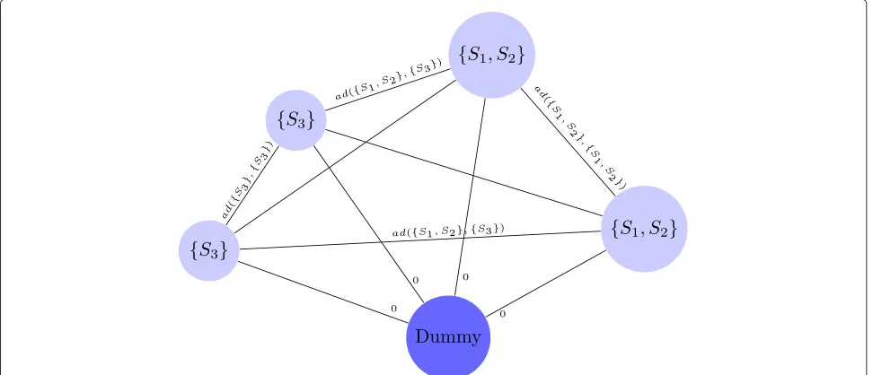
For an example, the example from Section “SFH” is continued. As stated in Section “Co-channel interference minimization”, the optimal solution from the first stage wasx{I1,I2} = x{I3} = 2 andxT = 0 for all otherT ⊆ S.
Thus,T := {{I1,I2},{I3}}. After calculating the induced adjacent channel interferencead({I1,I2},{I3}), the corre-sponding TSP instance is presented in Figure 2. There, each of the elements ofT demands two frequencies such that the corresponding vertices have to be copied two times.
A result of this example could be as follows.
Tour:Dummy→{I1,I2}→{I3}→{I3}→{I1,I2}→Dummy
Depending on the values ofad(Ii,Ij), this solution might
be optimal.
Figure 2Second Stage Problem as TSP.Example of the TSP formulation of the second stage problem.
graph, such that these implementations cannot be used straight forward. As a result, we stick to the sub-tour elim-ination formulation in this matter. The sub-tour elimina-tion formulaelimina-tion contains exponentially many constraints such that a separation approach is preferable. Separation of cutting planes means that the LP is only solved on a subset of all constraints. When a solution is available, it is checked whether an inequality is violated, which is in return added to the LP again and the process restarts. If no violated inequality exists, the LP-solution must be optimal. Similar as with the column generation approach, this concept helps to bypass memory limitations arising through exponentially many constraints. In fact, cutting planes and column generation are dual concepts. Again, the complexity of solving the LP relaxation depends on the computational complexity of the separating problem [21]. In this case, it can be solved, i.e., recognizing a violated sub-tour, in polynomial time. For more detailed information on cutting plane algorithms, we refer to [27].
In the context of MILP, cutting plane algorithms are mostly used to solve the linear relaxation of MILPs. For obtaining feasible integer solutions, it is necessary to com-bine cutting planes with a branching approach, i.e., every node is solved by cutting planes and it is then branched for integrality. Hereby, in any node different cutting planes might be added. On the whole, the combined method is calledbranch & cut.
Computational results
In the following, it is explained why the decomposition into two stages provides more meaning-full insights than the first formulation. Nevertheless, an optimal solution cannot be guaranteed.
Implementation details
The first stage problem [FAPH1] is degenerated. To be more precise, the problem can be treated by primal heuristics rather easily, because of the similarity to the classic FAP, but an optimal solution by a branch and price algorithm cannot be guaranteed. This is explained in the following and the two main reasons are pointed out. In general, there are two main problems, the first corresponds to the incorporation of priced variables and the second corresponds to the solution of the pricing problem.
are added successively until these correcting variables are all available. This may take arbitrarily many steps and is therefore not applicable for realistically sized instances. To our knowledge, no generic and efficient way of creating these correcting variables is known. In the following, we present some work around to this problem.
Given an improving variable, it is possible to cre-ate correcting variables heuristically. For this purpose, some modifications of construction heuristics, e.g., some DSATUR variation [19,28] suffice to create enough sur-rounding variables such that the improving variable can potentially have a value above zero in the next basic solu-tion. This means, given an improving variable, a totally new assignment based on this variable is created and the remaining variables are also added to the problem. Obviously, these surrounding variables may not form the best basic solution, with the priced variable contained, concerning the objective value. Further and especially concerning fractional solutions within the linear relax-ation, the surrounding variables may not allow to use the improving variable to its full extend, compared to the best possible usage. Additional, since every assignment con-tains|F| variables (compare constraint (6c)), adding one improving variable by adding|F| −1 others as well causes a certain inefficiency or redundancy. Consequentially, the solution process is slowed down. On the other hand, with these surrounding variables an improvement process can be constructed (see Section “Test results”), in which the improving variables are really used and at every pricing round, a primal solution is constructed. Hence, a pool of feasible integer solutions is generated which is a clear advantage over the [FAPSFH] formulation.
The second reason why no optimal solution can be claimed is the difficulty of the pricing problem. While it can be solved with reasonable effort at the beginning of the pricing process (e.g., by greedy heuristics) it gets increasingly hard to solve in the long run. Having variables in the order ofO(|S×S|)and only searching for a min-imum weighted (edge and node) subgraph makes up for a very difficult problem. As a result, the thorough solu-tion of the pricing-problem can slow down the solusolu-tion process significantly in the long run.
All in all, these are the two main reasons, why the tion process is slowed down, such that no optimal solu-tion, not even of the linear relaxation can be determined for most test instances presented in this article.
This slow performance is often observed in column generation algorithms. Measure for obtaining speedups are known as stabilization techniques, some of which are presented in [29]. In general, these techniques allow an LP solution to violate the constraint matrix as long as a sufficient penalty is payed. At the beginning of column generation, this offers more (and potentially better) dual solutions, while in the optimum, the penalties for violating
the constraints are too high, such that the optimum is the same as for the original problem. In our first stage problem, we assigned an additional “slack variable” (fre-quencies) to each constraint (6b), such that every STRX may use frequencies, not counting against the limit (6c) but with very high costs in the objective function. Con-sequentially, the pricing problem could be solved faster (at the beginning), such that there was no need for using heuristics only. On the other hand, the solutions started at a very high level of interference (compared to the original approach) and improved too slowly relative to the original approach, such that this stabilization techniques offered no significant gain.
Further stabilization techniques, e.g., presented in [30] advising alternative dual solutions for improving the pric-ing problem could not be used successfully either, since it is not trivial to find other dual solutions for our first stage problem. All in all, we are not aware of any stabi-lization techniques, significantly improving the first stage problem.
In addition to the problems presented above, no lower bounds or quality estimations on the linear relaxation can be provided. Like presented in [23], a lower boundlbon the linear relaxation can be computed by means of the current LP solutionx∗, the minimal reduced costs (the solution of the pricing problem)redx∗and an estimation
on the number of used (i.e., non-zero) binary variables|F| in each solution:
lb=x∗− |F| ·redx∗.
In a column generation framework, this lower bound converges (from below) to the optimum of the linear relax-ation (when the solution is optimal, the reduced costs are equal to zero). Nevertheless, this bound needs some fading-in before it can produce non-trivial results. This means thatlbcan be negative easily, while zero is a trivial lower bound in our problem. In our applications, no non-trivial results could be provided, for instances not being solved optimal. Hence, we are not able to give quality estimations on our primal solutions.
However, the second stage can be handled easier. The TSP instances in the second stage are very small with at most|F| +1 vertices. Hence, the TSP can be solved by the above formulation/separation approach. Contrary to the first stage, the second stage is solved optimally.
Test environment
The test instances have been taken from the COST256
Table 1 Overview scenario characteristics
Name STRX Available Freq.
100% 50% 150%
Siemens1 506 75 37 112
Bradford-0-Eplus 1886 75 37 112
Koeln 264 50 25 75
Swisscom 148 68 34 102
Overview on the used SFH-FAP instances. The second column describes the amount of STRXs, the third to fifth column denote the number of available frequencies.
The number of requested frequencies of each STRX (kI)
has been set to the number of inbound TRXs plus four since research on the gain of SFH indicates that most improvement can already be accomplished by a fixed amount of additional (to the number of inbound TRXs per STRX) channels [6]. Furthermore, the interference relations have been adapted as described in (1) and (2). Separation and blocking constraints have been omitted as reasoned in the beginning of Section “Decomposition into two stages”.
All computations were carried out on a 4x Intel(R) Xeon(R) CPU [email protected] GHZ machine with 12 GB RAM and a SCIP 2.11 implementation (with CPLEX 12.4 as underlying solver). Especially, this means that columns are subject to aging, such that SCIP may delete unused columns after a certain time. This is important, since cre-ating huge amounts of variables (because of the additional surrounding variables) would lead to a significant slow-down otherwise. However, the code has not been explicitly parallelized. As stop criterion a time limit of 100,000 s was set or until the available memory exhausted, depending on which condition occurred first.
Test results
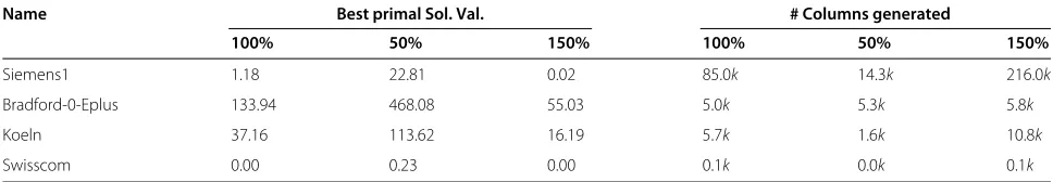
Concerning the first stage, general statistics on the lin-ear relaxation are given in Table 1. The second column describes the amount of STRXs and the third to fifth col-umn denote the number of available frequencies in three different cases. Further, Table 2 presents problem charac-teristics and solution values of its linear relaxation. The left numbers denote the amount of induced co-channel
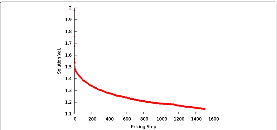
interference and the right numbers the amount of created variables (kfor 1,000). Additionally, Swisscom was solved optimal in all three versions while Bradford was aborted due to memory restrictions in the pricing problem. Hav-ing a closer look at statistics of the Siemens1 instance, the problems (degeneration) of the column generation approach become visible. As Figure 3 shows and like stated above, improving variables can be generated by solving [FAPHPR] during each pricing step. Adding these variables, together with heuristically generated correct-ing variables, can improve the objective function steadily (cf. Figure 4). Notably, both figures show a typical column generation behavior, i.e., a declining improvement. Never-theless, the solution process is far too slow (cf. Table 2). While relatively many variables need to be added (the improving and the correcting variables amount to at last
|F|additional variables per pricing step), the improvement rate is diminishing. Consequentially not even the optimal LP solution is reachable in most cases.
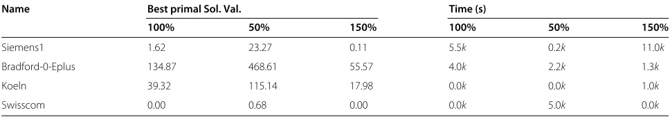
Nevertheless, because of the heuristic construction of surrounding variables, a range of primal solutions is cre-ated. The best, which are later passed to the second stage are presented in Table 3. There, the left numbers denote the amount of induced co-channel interference, the right numbers the time (in seconds) when the solution was found in the solution process.
Addressing the second stage, solution values are pre-sented in Table 4. Given the best available, feasible solu-tions from the first stage, the best solusolu-tions of the cor-responding second stage are reported. The left numbers denote the amount of induced adjacent channel inter-ference, the right numbers the percentage of adjacent channel interference with respect to the total interference. As mentioned before, the second stage can be formulated as a TSP problem such that a generally good solvability, especially on small instances can be claimed. Hence no deepening research is invoked here.
Even though the methodological research is in focus here, some general conclusions from our results are drawn in the following. For the instances Bradford, Koeln and Swisscom the adjacent channel interference is marginal compared to co-channel interference ln the quality of the decomposition approach. Only for the Siemens1 instance
Table 2 Overview on first stage results
Name Best primal Sol. Val. # Columns generated
100% 50% 150% 100% 50% 150%
Siemens1 1.18 22.81 0.02 85.0k 14.3k 216.0k
Bradford-0-Eplus 133.94 468.08 55.03 5.0k 5.3k 5.8k
Koeln 37.16 113.62 16.19 5.7k 1.6k 10.8k
Swisscom 0.00 0.23 0.00 0.1k 0.0k 0.1k
Figure 3Improving variables found.The number of improving (negative reduced costs) variables per pricing step for the first stage problem in the Siemens1 instance.
the adjacent channel interference is significant and an integrated approach might be beneficial.
Interference values are heavily dependent on the num-ber of STRXs as well as of the numnum-ber of available frequen-cies (combined with the particular interference relations). Obviously more STRXs lead to a higher amount of total interference while more frequencies reduce the interfer-ence. However, concerning computational effort it is to say that the amount of STRXs and the amount of frequencies
determine the difficulty of the first stage whereas the second is only dependent on the number of available frequencies.
In the following, we will shortly comment on the results of our approach in relation to other methods. Since we cannot provide a proof of optimality in most cases, we refer to Table 5 for a comparison between our results and results from a (exemplary) straight forward heuristic (for the first stage). These solutions are obtained by a direct
Table 3 First stage best primal solutions
Name Best primal Sol. Val. Time (s)
100% 50% 150% 100% 50% 150%
Siemens1 1.62 23.27 0.11 5.5k 0.2k 11.0k
Bradford-0-Eplus 134.87 468.61 55.57 4.0k 2.2k 1.3k
Koeln 39.32 115.14 17.98 0.0k 0.0k 1.0k
Swisscom 0.00 0.68 0.00 0.0k 5.0k 0.0k
The objective value of the best known integer solutions. The left numbers denote the amount of induced co-channel interference, the right numbers the time (in seconds) when the solution was found in the solution process.
greedy (DSATUR) heuristic for the first stage problem and then processed by the second stage. As one can see, the results obtained by the means of mixed integer program-ming are always better in the first stage. Because of the two staged approach, a better first stage solution does not correspond to a better second stage solution, such that the same cannot be claimed for the second stage. Nev-ertheless, only one instance was solved worse and the overall solution of both stages is always but one time bet-ter than the solutions produced by the greedy method in the first stage. However, this can obviously not be claimed for all heuristics, but this emphasizes the viability of mixed integer programming for such problems. Especially since each heuristic can be incorporated into a mixed inte-ger programming approach, combining the strength of both approaches.
Comparison to FAP
At the beginning of this article, SFH was introduced and motivated on the background of the standard FAP. In this section, the above-presented results are related to the results of FAP, presented at [18]. Both prob-lems are similar and produce interference results. How-ever, these interference amounts are not straight forward comparable. Without going into technical details, SFH benefits from frequency- and interference-diversity and in the end of error recognition codes. Especially this means, that SFH networks can have single time-frames on single connections with very high interference with-out harming the overall speech quality, as long as the other time-frames offer a connection “good enough”. The
incorporation of random effects offers a gain towards the classic FAP beyond the pure measure of interference. However, this randomization formally leads to higher interference amounts of the assignment, regarding total numbers. This is explained in the following.
The FAP considers an optimal, overall assignment in every time-frame. In slow-frequency hopping, the assign-ment is changed at every time-frame, resulting in most time-frames not having optimal assignment. Every single frame is equal or worse compared to each FAP time-frame, concerning interference values but no frequency hopping gains. Consequently, the total expected interfer-ence in SFH-Networks must be higher compared to FAP networks. This can be illustrated by the following exam-ple: Consider the “tiny” instance from the FAP website, with the frequency spectrum set to{5,. . ., 11}and thekI
values set to one (equal to FAP) and three, respectively. This leads to the following solutions:
Solutionk=1 :
x1,6,7=x3,4=x3,4,5=x7=1, x2=3 Interference =0;
Solutionk=3 :
x2=x2,3=x3,4=1, x1,2,6,7=x3,4,5=2 Interference =2·Co({1, 2, 6, 7})+1
×co({2, 7})=2·0.03+0.03=0.09
Obviously the instance wherek=1 has a lower frequency reuse factor, the average set size of STRXs sharing a fre-quency is smaller compared to the other case. Since the
Table 4 Overview second stage results
Name Best primal Sol. Val. % of total interference
100% 50% 150% 100% 50% 150%
Siemens1 3.17 9.83 1.37 0.66 0.30 0.93
Bradford-0-Eplus 8.34 20.78 4.33 0.06 0.04 0.07
Koeln 1.11 3.46 0.42 0.03 0.03 0.02
Swisscom 0.00 0.00 0.00 - 0.00
Table 5 Direct heuristic results
Name Frequencies First stage Second stage Total greedy Total pricing
Siemens1 75 1.98 3.39 5.37 4.79
Siemens1 37 24.12 10.01 34.13 33.10
Siemens1 112 0.18 1.24 1.42 1.48
Bradford 75 140.82 8.79 149.61 143.21
Bradford 37 470.51 20.32 490.83 489.39
Bradford 112 56.79 4.29 61.08 59.90
Koeln 50 40.36 1.13 41.49 40.43
Koeln 25 116.23 3.36 119.69 118.60
Koeln 75 19.18 0.42 19.60 18.40
Swisscom 68 0.00 0.00 0.00 0.00
Swisscom 34 1.04 0.00 1.04 0.68
Swisscom 102 0.00 0.00 0.00 0.00
Comparison to results obtained by a straight forward greedy-heuristic for the first stage. The overall best results per instance have been marked bold.
chance of interference rises quadratically in the amount of STRX in a single set, the overall interference level rises (though every single potential interference value is strictly lower) ifkincreases. In other words, with a relatively low k value it is possible to form sets of STRX having very few (if any) interference relations not equal to zero while at higherk values, i.e., demanding more frequencies to hop, increases the set size and therefore the chance of strictly positive interference values dramatically. In the above context, this means that inducing randomization will increase the probability of having a suboptimal assign-ment in one time-frame, thus increasing the expected interference.
In consequence, more (positive) interference values are taken into account in SFH compared to FAP. Although FAPH has smaller interference values per “link”, see (1) and (2), this leads to an overall higher number of expected interference, therefore making a comparison by pure interference values misleading.
Conclusions
Drawing a final conclusion on the presented research, the concept of SFH-FAP can be modeled by means of mixed integer programming, similar to the classical FAP. Nev-ertheless, realistically sized instances cannot be solved and demand for more sophisticated approaches. Here, a decomposition into two stages was proposed such that the huge size of the problems can be engaged by a col-umn generation and separating approach, respectively. While this decomposition does not allow to obtain opti-mal results in the first stage, by a sensible implementation, a range of primal solutions/assignments could be pro-duced which can be passed on to the second stage so that the assignment can be finalized there. However, the prob-lem is extremely hard so solve, as well in the perspective
of complexity theory as by practical aspects. Exponen-tially many variables lead to column generation, whereas the pricing problem is, because if its generality, very hard to solve. The solutions of the pricing problem are (even with stabilization techniques) not trivially incorporated into the first stage problem, such that the improvement rate is very slow and the optimum is not reachable.
Since the obtained results are not optimal, the whole effort has a heuristic character, only. Hence, this approach might be, because of the rather high computational effort, inferior to a straight forward heuristic solution with-out invoking the means of mixed integer programming. Although we cannot claim an optimal solution, the bottle-neck of this approach could be pointed out, namely a (fast) solution of the pricing problems as well as the incorpo-ration of newly priced variables into new basic solutions. Future research, which bypasses this problem, could lead to an optimal solution of the first stage such that the com-plete frequency assignment in SFH networks could be done evidently close to optimal.
Competing interests
Both authors declare that they have no competing interests.
Received: 15 February 2012 Accepted: 25 July 2012 Published: 14 August 2012
References
1. ST Chung, A Goldsmith, Degrees of freedom in adaptive modulation: a unified view. IEEE VTS 53rd Veh. Technol. Conf.2, 1267–1271 (2001) 2. X Qiu, K Chawla, On the performance of adaptive modulation in cellular
systems. IEEE Trans. Commun.47, 884–895 (1999)
3. L Toni, A Conti, Does Fast Adaptive Modulation Always Outperform Slow Adaptive Modulation? IEEE Trans. Wirel. Commun.10, 1504–1513 (2011) 4. H Bogucka, A Conti, Degrees of freedom for energy savings in practical
adaptive wireless systems. IEEE Commun. Mag.49, 38–45 (2011) 5. M Chiani, A Conti, R Verdone, Partial compensation signal-level-based
6. H Olofsson, J Naeslund, J Skold, Interference diversity gain in frequency hopping GSM. 45th Veh. Technol. Conf.1, 102–106 (1995)
7. M Chiani, E Agrati, O Andrisano, An analytical approach to evaluate service coverage in slow frequency-hopping mobile radio systems. IEEE Trans. Commun.49(8), 1447–1456 (2001)
8. M Chiani, A Conti, O Andrisano, Outage evaluation for slow
frequency-hopping mobile radio systems. IEEE Trans. Commun.47(12), 1865–1874 (1999)
9. KI Aardal, CPM van Hoesel, AMCA Koster, C Mannino, A Sassano, Models and solution techniques for the frequency assignment problem. Ann. Oper. Res.153, 79–129 (2007). doi:10.1007/s10479-007-0178-0 10. B Jaumard, O Marcotte, C Meyer, T Vovor, Comparison of column
generation models for channel assignment in cellular networks. Discrete Appl. Math.112(1-3), 217–240 (2001)
11. B Jaumard, O Marcotte, C Meyer, T Vovor, Erratum to “Comparison of column generation models for channel assignment in cellular networks”. Discrete Appl. Math.118(3), 299–322 (2002)
12. TD Hemazro, B Jaumard, O Marcotte, A column generation and branch-and-cut algorithm for the channel assignment problem. Comput. Oper. Res.35(4), 1204–1226 (2008)
13. A Mehrotra, M Trick, A column generation approach for graph coloring. INFORMS J. Comput.8(4), 344–354 (1995)
14. J Moon, L Hughes, D Smith, Assignment of frequency lists in frequency hopping networks. IEEE Trans. Veh. Technol.54(3), 1147–1159 (2005) 15. T Nielsen, J Wigard, PH Michaelsen, P Mogensen, Resource allocation in a
frequency hopping PCS1900/GSM/DCS1800 type of network. 49th IEEE Veh. Technol. Conf.1, 209–214 (1999)
16. P Bj ¨orklund, P V¨arbrand, D Yuan, Optimal frequency planning in mobile networks with frequency hopping. Comput. Oper. Res.32, 169–186 (2005) 17. M Tieves, Frequency assignments in slow frequency-hopping gsm
networks-a MIP approach. Master’s thesis, RWTH Aachen, (2011). http:// www.math2.rwth-aachen.de/de/forschung/publ
18. A Koster, A Eisenbl¨atter. http://fap.zib.de, 2001–2012
19. A Eisenbl¨atter, Frequency assignment in GSM networks: models, heuristics, and lower bounds. PhD thesis, TU Berlin, 2001
20. A Mehrotra, M Trick, inExtending the Horizons: Advances in Computing, Optimization, and Decision TechnologiesA branch-and-price approach for graph multi-coloring. (Springer, New York, 2007), pp. 15–29
21. M Gr ¨otschel, L Lov´asz, A Schrijver,Geometric Algorithms and Combinatorial Optimization, Volume 2 of Algorithms and Combinatorics(Springer, New York, 1988)
22. D Johnson, M Garey,Computers and Intractability: A Guide to the Theory of NP-Completeness(W. H. Freeman, San Francisco, 1979)
23. G Desaulniers, J Desrosiers, M Solomon,Column Generation(Springer, New York, 2005)
24. D Applegate, R Bixby, V Chvatal, W Cook,The Traveling Salesman Problem (Princeton University Press, Princeton, NJ , 2006)
25. T Achterberg, T Berthold, Scip tsp example. http://scip.zib.de/doc/ examples/TSP/index.html
26. Concorde Solver. http://www.tsp.gatech.edu/index.html
27. L Wolsey,Integer Programming(John Wiley and Sons, New York, 1998) 28. D Br´elaz, New methods to color the vertices of a graph. Commun. ACM.
22, 251–256 (1979)
29. O Du Merle, D Villeneuve, J Desrosiers, P Hansen, Stabilized column generation. Discrete Math.194, 229–237 (1999)
30. M Leitner, M Ruthmair, G Raidl, On stabilizing branch-and-price for constrained tree problems. Technical Report, Institute of Computer Graphics nad Algorithms, Vienna, 2011
doi:10.1186/1687-1499-2012-253
Cite this article as:Koster and Tieves:Column generation for frequency assignment in slow frequency hopping networks.EURASIP Journal on Wire-less Communications and Networking20122012:253.
Submit your manuscript to a
journal and benefi t from:
7Convenient online submission
7Rigorous peer review
7Immediate publication on acceptance
7Open access: articles freely available online
7High visibility within the fi eld
7Retaining the copyright to your article