Volume 2010, Article ID 901283,17pages doi:10.1155/2010/901283
Research Article
Localization in Wireless Sensor Networks with
Known Coordinate Database
Zhen Fang,
1Zhan Zhao,
1Xunxue Cui,
2Daoqu Geng,
1, 3Lidong Du,
1, 3and Cheng Pang
1, 31State Key Laboratory of Transducer Technology, Institute of Electronics, Chinese Academy of Sciences, Beijing 100190, China 2New Star Research Institute of Applied Technology, Hefei 230031, China
3Graduate University of Chinese Academy of Sciences, Beijing 100039, China
Correspondence should be addressed to Zhen Fang,[email protected]
Received 24 December 2009; Revised 23 April 2010; Accepted 3 June 2010
Academic Editor: Davide Dardari
Copyright © 2010 Zhen Fang et al. This is an open access article distributed under the Creative Commons Attribution License, which permits unrestricted use, distribution, and reproduction in any medium, provided the original work is properly cited.
Geographic location of nodes is very useful for a sensor network. A novel and practical Radio Frequency (RF)-based localization algorithm called Kcdlocation has been presented for some specific sensor network topologies, such as the grid and linear types. The Kcdlocation algorithm is adapted to those wireless sensor networks deployed with known coordinate database. It examines the ordered sequence of neighboring unknown nodes relative to some anchor nodes so that they are ranked to compute the location of unknown nodes by wireless localization measurements. After the task of distinguishing neighboring unknown nodes is completed through the ranging technology, the correct position for each sensor node would be identified. The localization scalability and fault tolerant performance of this algorithm have been evaluated from the perspective of practicability. Its performances for the real circumstance are verified through different experiments with several RF channels and deployment parameters. The node localization accuracy of Kcdlocation in a 5∗4 grid network reaches 100% in a flat open square.
1. Introduction
Wireless Sensor Networks (WSNs) have been recently pro-posed for a multitude of diverse applications to acquire and process information. Node localization is an important enabling technology for the deployment of sensor networks in a wide variety of applications. It refers to the process of determining the position of every sensor. Their locations are known in advance by some deployed nodes, which are called anchors. Other nodes compute their locations based on those anchors.
The localization/positioning problem has been an active research area for the last few years, which can be traced back to early node positioning for personal mobile computing. Localizing sensors is necessary for many sensor network applications such as tracking, monitoring, and geometric-based routing [1].
The problem of node localization has been researched and evaluated through simulations. If some strict hard-ware constraints are imposed on wireless sensor nodes, real system implementations for some proposed solutions
would not bring encouraging results [2]. Many people take the method of estimating relative distances between sensor nodes—RF signal strength indication (RSSI) such that they would largely fail in practice, as a result of the presence of multipath fading and shadowing in the RF channel [3, 4]. If a localization algorithm is robust to the randomness of the radio communication, it would require a good calibration scheme together with the localization process, which is less sensitive to abnormal radio pat-tern.
For this kind of network model with a known coordinate database, it is not convenient to preprogram all sensor nodes with their respective coordinates before deployment, as it may be time consuming and tedious to manually program a large number of nodes with different deployment coordinates, and then deploy each node at the actual position corresponding to the preprogrammed deployment coordinates. Furthermore, it would often make mistakes in the deployment process. A usually familiar fact is that the monitoring area would be altered and the nodes may be physically reprogrammed with their new deployment coordinates.
There are many application scenarios with a known coor-dinate database in sensor networks. For example, soldiers would deploy their sensor network on a ground battlefield to achieve the defense and reconnaissance function in an unmanned watching manner by using this kind of sensor network. These detection networks are usually designed as a fine-grid form in order to implement the rigorous surveillance on the hostile district [6].
Moreover, grid sensor networks are often deployed for the precision agriculture application [7,8]. For the control and management of greenhouses and field farms, a large-scale planting area is divided into many regular grids to obtain the environmental parameters such as temperature, humidity, and solar radiation. An important issue that arises in precision agriculture is the node position to be sensed. Thus, a position computation approach should be provided for the large-scale environmental measurements [9].
Based on the aforementioned points for network deploy-ment, we propose a novel and practical RF-based localization algorithm for WSN with known coordinate database. This solution is fit for the case where the goal of sensor network deployment is grid and linear topology. Linear topology is a simple sensor system where a set of nodes are placed along straight lines. These network models are enlightened by our assumption, where a realistic deployment of a sensor network is not random, and an approximation to a uniform or even grid distribution is expected. It is easy to visualize the practical scenes from farmland to playground environmental monitoring, where the deployment of sensor nodes is preplanned orderly, and the model of sensor networks has the grid character.
As our localization algorithm is designed for the sensor network model with known coordinate database, it is named as “Known Coordinate Database for Localization”, that is, “Kcdlocation” for short. To the best of our knowledge, we are the first to use RSSI to realize localization in wireless sensor networks with a known coordinate database.
The main process of Kcdlocation algorithm is provided as follows: the ordered sequence is examined for neighboring unknown nodes with unknown locations relative to anchor nodes, and then the knowledge is adopted about known coordinate database that has been saved in each node to determine the location of unknown nodes. The ordered sequence of unknown nodes is obtained by ranking them based on RSSI measurements.
Theoretically, the ranks of the unknown nodes based on RSSI readings should be monotonic with their ranks of
Euclidean distances; however, this is not true in the real world because of the unreliable nature and irregular pattern of the radio communication. Considering that the signal propagation model that maps RSSI values onto distance is the log-normal model, each localization step will only localize unknown nodes within one hop to mitigate the effects of irregular radio. Once RSSI ranging technology distinguishes neighboring unknown nodes relative to anchor node within one hop, Kcdlocation can achieve the accurate position of an unknown node. The experimental results have shown that the localization accuracy by Kcdlocation reaches 100% in obstacle-free environments.
The rest of this paper is organized as follows.Section 2 presents related localization work in wireless sensor net-works.Section 3contains the central part of the paper where the Kcdlocation algorithm is described. The performance evaluation and simulation is provided in Section 4. In Section 5, the Kcdlocation performances for real system are verified through various experiments. Finally, our conclu-sions are obtained.
2. Related Work
Sensor positioning is a fundamental and crucial issue for network operation and management. Localization systems are classified into two categories: range-based algorithms and range-free algorithms. Range-based algorithms estimate distances and/or angle between the unknown nodes and the anchor node, while range-free algorithms exploit radio connectivity to confirm proximity or exploit the sensing capabilities of each sensor [10,11].
Range-based techniques should estimate distance using different methods such as time of arrival (ToA) [12–14], time difference of arrival (TDoA) [12, 15, 16], angle of arrival (AoA) [12,17], and RSSI [2,3,18–26], and then use distance to triangulate the location of unknown nodes. All the four distance measurement methods except RSSI have superior measuring precision, thus range-based techniques produce fine-grained locations.
As the effects of reflecting and attenuating objects in an environment have much larger influences on RSSI than on distance, the reputation of RSSI is too unpredictable for range estimation [3,4]. Nevertheless, as described in many papers, the RSSI with low-power radios can be applied to the direct distance estimation in an ideal open and outdoor environment. The experimental outcome demonstrates that, under the appropriate conditions, RSSI localization is a feasible alternative to localization like GPS [3].
The AHLoS system uses iterative multilateration which relies on a small set of nodes initially configured as beacons to estimate node locations in an ad hoc setup [14]. The algorithm employs the ranging technique of Time of Arrival (ToA) that requires extensive hardware and solves a relatively large nonlinear system of equations.
Unlike most range-based localization methods, Kcd-location algorithm does not directly utilize the ranging technique. It uses RSSI to evaluate the neighboring unknown nodes and decide who is further or closer to the anchor node. Consequently, Kcdlocation is a range-free rather than ranged-based algorithm. It does not require any infrastruc-ture, thus it is an absolutely decentralized algorithm.
Due to the hardware cost of radio, sound, ultrasound, or infrared signals, as well as the strict requirements on time synchronization and energy consumption, it is hard to expect cheap, unreliable, and resource-constraint sensor nodes to make use of range-based localization methods in practice. To overcome the limitations of the range-based localization schemes, many range-free methods had been proposed. Several representative range-free algorithms are presented below.
In [27], a centralized technique using convex optimiza-tion is developed to finish the localizaoptimiza-tion process based on connectivity constraints given some nodes with known positions. MDS-MAP [28, 29] improves on these results by using a multidimensional scaling approach based on centralized computation.
In [30], a globally rigid Delaunay complex is constructed for localization in a large sensor network. The work in [31] is a follow-up of [30] where an incremental method is proposed to select landmarks such that the combinatorial Delaunay complex is rigid and represents the sensor field shape, which is then used for anchor-free connectivity-based localization.
As a decentralized algorithm, the DV-Hop method [32] calculates the node position based on the received anchor locations, the hop count from the corresponding anchor, and the average distance per hop obtained through anchor communication. Similarly, the Amorphous Positioning algo-rithm proposed in [33] uses offline hop-distance estimations, and improves location estimates through a way of neighbor information exchange.
The Echolocation method [18] determines the location of unknown nodes by examining the ordered sequence of received signal strength measurements taken at multiple reference nodes. The key idea of this method is that the distance-based rank order of reference nodes constitutes a unique signature for different regions in a localization space. For Probability Grid method [2], a location estimation scheme is applied to its positioning procedure, which takes a probabilistic approach to estimate the node location and uses the additional knowledge of topology deployment.
The main idea of the Spotlight localization system [10] is that the controlled events are generated in the field where the sensor nodes are deployed. Using the time when an event is perceived by a sensor node and the spatial-temporal properties of the generated events, spatial information (i.e., location) regarding the sensor node can be inferred.
In addition to the range-free localization schemes described above, some similar algorithms have been pro-posed, such as RIPS [34], Resilient LSS [35], KPS [36], LAD [37], APIT [38], MSP [39], APL [40], StarDust [41], and Rendered Path [42].
Our method is significantly different from the existing methods. According to some practical scenarios, we conclude that these sensor networks are deployed in a controlled man-ner, where the aim of deployment is to form specific topolo-gies, and the accurate deployment knowledge is obtained after deployment. With the deployment knowledge in those topologies, the Kcdlocation would be easy to be deployed, and would provide relatively high localization precision, low cost, and small energy consumption. However, the Kcdlo-cation is not intended to replace the existing localization methods, as it requires an accurate modeling of deployment knowledge and adapts to these specific network topologies.
3. Kcdlocation Algorithm
The Kcdlocation algorithm examines the ordered sequence of unknown nodes relative to an anchor node, by ranking those nodes based on RSSI measurements between them and the anchor node to determine the locations of unknown nodes. Once the ranging technology can distinguish neigh-boring unknown nodes, the algorithm will identify the correct position for each sensor node. Whether neighboring unknown nodes can be distinguished or not depends on the precision of ranging technology and distances between the nodes, and the latter factor is largely determined by network topology map. To estimate the correct position of each node, a good tradeoff between ranging technology and distance between the nodes should be achieved. Considering that RSSI distance estimation, which has relatively low precision of ranging, is used in Kcdlocation to distinguish neighboring nodes, the Kcdlocation will be suitable for these specific topologies, where the distance between any two neighboring nodes is regular rather than arbitrary. Unless otherwise noted, we use the grid topology in the remainder of this paper to describe Kcdlocation algorithm.
Figure 1 illustrates the network model of known coor-dinate database for a simple case of the M∗N unknown nodes. The gray square represents unknown node, and the black square represents anchor node. Each node is randomly deployed in grids and stores the information of a coordinate database corresponding to deployment grids.
With the increase of network size, the limited storage capacity implies that the entire coordinate database is a heavy load for each sensor node. However, the location coordinate database corresponding to such simple network topology, as described in Figure 1, can be expressed as boundary conditions (coordinates of four vertexes) and grid distance.
U1
Figure1: Schematic example of Kcdlocation algorithm.
As shown inFigure 1, an anchor node (A) is placed in the grid, and its location is (1, 0) length unit, where there are two unknown nodes (U1andU2)which are nonequidistant with the anchor nodeAwithin one hop.
For each node in the grid topology, we assume that the effective range of one hop is √2R, that is, diagonal grid distance (Ris grid distance), thus the number of neighboring nodes within one hop is not more than eight. Considering that the RSSI distance measurement has relatively higher precision in a short range [3,4], each localization unit only considers the neighboring unknown nodes within one hop so as to distinguish neighboring unknown nodes correctly. The goal of the Kcdlocation algorithm is to estimate the correct position in the grid for each sensor node. The localization error may arise from an incorrect positioning for each sensor node in the grid, because of the precision of distance measurement based on RSSI below the threshold that can distinguish neighboring unknown nodes.
The basic principle of the algorithm is that after the anchor node receives localization request messages from the neighboring unknown nodes, it compares the RSSI values corresponding to the neighboring unknown nodes to distinguish the relative distances, and then accomplishes the localizing task for the neighboring unknown nodes based on the foundation of known coordinate database. The Kcdlocation algorithm is an orderly advanced flooding algorithm. It is first launched by the deployed anchor node to finish the localization computation task for its neighboring unknown nodes, and then the procedure advances outward sequentially to complete the whole network’s localization. Once an unknown node has localized its position, it becomes an anchor node and helps the neighboring unknown nodes localize. This process is repeated until as many unknown nodes as possible accomplish their locations.
The Kcdlocation algorithm is carried out by iterative procedure which uses the atomic localization model as a basic unit and the collaborative localization model as an additional enhanced unit. The atomic localization unit, the collaborative localization unit, and the localization iterative process will be described in the following paragraphs.
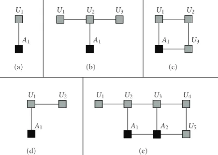
3.1. Atomic Localization. Atomic localization makes up the basic case where one or two unknown nodes can estimate their correct grid locations when they are within one hop around an anchor node and meet the appropriate requirement described below. Atomic localization can be broadly classified into four main types, as shown in Figures 2(a),2(b),2(c), and2(d). The black squares represent anchor nodes, and the gray squares represent unknown nodes.
Here all unknown nodes broadcast periodic localization request messages, which consist of a tuple of the format {message identifier, sourceID, and powerLevel}. Message identifier identifies the message function; sourceID is the unique identifier of the unknown node; powerLevel is the transmission power level used to broadcast the localization request message.
The original anchor node and subsequent localized nodes listen for some period of time to acquire a signature, which consists of the set of localization request messages received over some time interval, and then calculate the mean RSSI of a set of localization request messages corresponding to the identical unknown node. Each mean RSSI is mapped onto an unknown node using a specific powerLevel. Using mean RSSI and multiple transmission power level can decrease the effect of multipath fading and shadowing in the RF channel during the RSSI distance measurement.
According to the detailed RSSI value, the anchor nodes conclude the number of unknown nodes around themselves within one hop and judge whether there are unknown nodes meeting the appropriate requirement as described in Figures 2(a), 2(b), 2(c), and 2(d). The unknown nodes meeting localization requirement can estimate its location with the help of neighboring anchor nodes. Once an unknown node estimates its grid position, it will change into an anchor node and broadcast its estimated grid position to neighboring nodes, which enable them to know the state of localization of neighboring nodes.
Let the deployment of unknown nodes be in a grid topology of dimensionsM ∗N shown in Figure 1. Let U
be the set of all unknown nodes in the sensor network such that each unknown node can be represented byUi, for
i =1,. . .,m∗n. We takeGi(its coordinates (xi,yi)) as the corresponding deployment point, and letGbe the set of all
Gicoordinates stored in sensors’ memories.
For each localization unit, only nodes within one hop are considered.Direpresents the set of coordinates within one hop of the anchor nodeAi, whose coordinates are (xi,yi).Di is expressed as follows:
In Figure 2(a), there is only one unknown node U1
around the anchor node A1 within one hop. When the anchor nodeA1detects the above type according to RSSI, it assigns the only grid coordinate that is not deployed around
A1within one hop to the unknown nodeU1.
U1 U1 U2 U3 U1 U2
A1 A1 U3
A1
U1 U2 U1 U2 U3 U4
A1 A1 A2 U5
(a) (b) (c)
(d) (e)
Figure2: Schematic illustration of atomic unit and collaborative unit.
anchor nodeA1. This can be concluded from the relation between RSSI and distance
RSSIi>RSSIj=⇒di< dj. (2)
Here, RSSIi and di are the RSSI measurement and distance between an anchor node and its neighboring unknown node, respectively.
From the above equation, it can be inferred that the unknown node corresponding to maximum RSSI should be the nearest node to the anchor node, that is, the unknown node U2 is the nearest member to the anchor node A1. According to theD1(the set of coordinates within one hop of the anchor nodeA1) and the localization state of neighboring nodes, the grid coordinate that is nearest to the anchor node
A1within one hop and not deployed should be assigned to the unknown nodeU2.
The localization approach of Figure 2(c) is similar to Figure 2(b), however, for this condition the localizable unknown node U2 corresponding to the minimum RSSI is farthest to the anchor node A1. In this scenario, the undeployed grid coordinate which is farthest to the anchor nodeA1within one hop should be assigned to the unknown nodeU2according to the above localization deduction.
InFigure 2(d), there are two unknown nodes (U1,U2) around the anchor nodeA1 within one hop, where the dis-tances among the two unknown nodes and the anchor node are grid distance (R) and diagonal grid distance, respectively. When the anchor nodeA1receives localization request mes-sages corresponding to different RSSI transmitted from two unknown nodes within one hop, by calculating Manhattan distance between the two undeployed grid coordinates and
A1 (coordinates (x1,y1)), respectively, the undeployed grid coordinate with the less Manhattan distance is assigned to unknown nodeU1, which corresponds with higher RSSI, and vice versa. The Manhattan distance is expressed as follows:
M(Ui,A1)= |xi−x1|+yi−y1. (3)
Here,Ui represents an unknown node and (xi,yi) is its corresponding coordinate. The Euclidean distance can be used as well, but Manhattan distance is very efficient to compute over nodes with low computational capabilities, though they both produce similar results.
3.2. Collaborative Localization. The Kcdlocation algorithm adopts atomic localization as its basic unit to estimate the correct position in the grid network. In a deployment with regular grid distribution of nodes, as shown in Figure 1, it is highly possible that at some nodes the conditions for atomic localization would not be met, that is, two or more unknown nodes are equidistant with the anchor node, therefore it is not able to localize their position through atomic localization.
Figure 2(e) illustrates one of the most common topolo-gies for which the collaborative localization model can be applied. The anchor node A1 has three neighboring unknown nodes (U1,U2,U3), two of which are equidistant with A1, and one of which is the nearest to A1. The anchor node A2 has four neighboring unknown nodes (U2,U3,U4,U5), where unknown nodes (U2,U4) are equidis-tant withA2, and the distance is diagonal grid distance while the other two unknown nodes (U3,U5) are equidistant with
A2, and the distance is grid distance. Under this condition, the unknown nodes (U1,U2,U3,U4,U5) can localize their coordinates by collaborating with anchor nodesA1andA2. We refer to it as collaborative localization.
The collaborative localization procedure can be started as follows: the first step is performed by the anchor node
A1, where the nearest unknown nodeU2 can be localized. Then the anchor nodeA2 has three neighboring unknown nodes (U3,U4,U5); one of which is farthest to the anchor node. This circumstance is identical to Figure 2(c) type, therefore the farthest node U4 can be localized. And then the two neighboring anchor nodes A1 and A2 have two equidistant unknown nodes, respectively. Therefore, it will not be able to determine these unknown nodes’ positions by atomic localization. When this occurs, by exchanging messages between the two neighboring anchor nodesA1and
A2, it can be determined that the unknown node (U3) is the only unlocalized neighboring node of the two anchor nodes, and distances betweenU3and the two anchor nodes are diagonal grid distance and grid distance, respectively. The grid coordinates belong to the intersection set of coordinates within one hop of the two anchor nodes and meet the distance requirement, thus it can be assigned to nodeU3. The undeployed grid coordinates can be written as follows:
xi,yi
∈D1∩D2∩di1=
√
2·R∩(di2=R)
∀i∈undeployed coordinates indexes, (4)
Algorithm Kcdlocation
Initialization: unknown nodes broadcast localization request messages (LRM) periodically; anchor nodes listen for some period of time to detect the number of unknown nodes (Mi) around themselves within one hop.
Procedure:
/∗detect neighboring unknown nodes ( )∗/ for all anchor nodesAj, (1≤j≤n)
while(Ajreceives LRM) {if(Ajreceives identical LRM)
Ajcalculate mean of RSSI corresponding to identical unknown node.
else {Mi++.}}
/∗anchor node detectsM
ifor some period of time∗/
/∗unknown nodes localization ( )∗/
switch(Mi) /∗atomic localizaion∗/
{ case1: this type is same asFigure 2(a). break;
case2:if(unknown nodes have different RSSI) {this type is same asFigure 2(d).}
else { } break;
case3:if(one unknown node has different RSSI compared with others)
{this type is same asFigure 2(b) orFigure 2(c).}
else { } break;
case4: break;
case5: break;
default:; }
/∗During the iterative process of localization, when the requirement for atomic unit is not meet, the algorithm could call collaborative unit to accomplish localization.∗/
/∗According to the principle of Kcdlocation, the maxMiis not more than five. IfMiis more than three, it is
impossible that one unknown node has different RSSI compared with others for connectivity of grid network.∗/
Algorithm1: Flowchart of Kcdlocation algorithm.
If two adjacent anchor nodes share common one or two unknown nodes in their neighborhood, these nodes can initiate a collaborative localization procedure. Collab-orative localization provides help in situations where the requirement for atomic localization is not satisfied. By collaborating with neighboring anchor nodes and orderly using atomic localization unit, unknown nodes can be localized in collaborative localization circumstance, thus collaborative localization is very important complement of atomic localization.
3.3. Algorithm Iterative Process. The Kcdlocation iterative process uses atomic localization as a basic unit and collab-orative localization as a complement unit to estimate node locations. This localization algorithm is an orderly advanced flooding procedure, which launches by the initial deployed anchor node. The anchor nodes detect the neighboring unknown nodes within one hop by RSSI corresponding to unknown nodes transmitting localization request message, and then accomplish the unknown nodes localization which meets the localization requirements illustrated inFigure 2.
When an unknown node estimates its grid location, it becomes an anchor node and helps the neighboring unknown nodes to be localized. The process is repeated until the positions of as many unknown nodes as possible in a grid topology are estimated. The flowchart of the Kcdlocation algorithm is shown inAlgorithm 1.
An example is provided to explain the Kcdlocation algorithm in more detail. As shown inFigure 1, the originally deployed anchor node A launches the whole network localization. First, the unknown nodes U1 and U2 within one hop of anchor node A can be localized with the help of A. Neighboring node U1 has only two unknown nodes (U3 and U4) which are not equidistant with U1, but around node U2 there are four unknown nodes (U3,
U4, U8, and U9), thus the second step is only launched by U1, and unknown nodes (U3 andU4) can be localized. Now, there are three anchor nodes (U2, U3, and U4) in the neighboring region of unknown nodes, where unknown nodes (U5 and U6) are within one hop of U4 while unknown nodes (U8andU9) are within one hop ofU2, and neighboring U3 has five unknown nodes (U5,U6, U7,U8, andU9). According to the localizable decision rule described above, only anchor nodeU2 andU4 can help neighboring unknown nodes localize, thus unknown nodes U5, U6,
U8, and U9 can be positioned. Finally all the unknown nodes are localized in the light of the above localization principles.
The problem of iterative process is the error accumula-tion resulting from the use of unknown nodes that estimate their positions as anchor nodes. The failure of a node could make negative effects on Kcdlocation. If the failure node is next to the starting anchor, the localization could be compromised. Fortunately, this error accumulation is a trivial problem because of the relatively low requirement of distance measurement precision in Kcdlocation. Most of the ranging technologies such as RSSI can meet the requirement of ranging precision in Kcdlocation, which are only used to distinguish the neighboring unknown nodes relative to an anchor node in a grid topology within one hop.
Moreover, the accuracy of those localized nodes can be verified in the process of the localization. Once the position of an unknown node has been determined, especially for the node with neighboring unknown nodes to be localized, through exchanging the positions’ information with the neighboring localized nodes, it can acquire the position information of its neighboring localized nodes. This is served as an accuracy reinforcement process of node localization and can eliminate some cases where multiple nodes localize themselves to the same position in the grid. If the unknown node Ui has obtained the correct position (xi,yi), the coordinates of its neighboring localized nodes should be the subset ofDi, which is the set of coordinates within one hop of the localized position (xi,yi) and can be derived from (1) in this paper. Otherwise, the coordinates (xi,yi) are not the real position for the unknown node Ui. To avoid the error accumulation in the localization process, the localized unknown nodeUi is suspended, and not taken as the kind of anchor node to help the neighboring unknown nodes. The mistaken localization node Ui can broadcast periodic localization request messages and relocate its position. The verification solution we mentioned above could still require further refining to provide a better applicability and effectiveness.
4. Performance Evaluation
A complete performance of Kcdlocation has been evaluated from the viewpoint of algorithm practicability including three issues: anchor node placement, localization scalability, and localization tolerance and performance simulation.
4.1. Anchor Node Placement. The Kcdlocation algorithm is started from an anchor node on the periphery of the network, and location information is propagated to other nodes in the network. Once the ranging technology can distinguish neighboring unknown nodes, the algorithm will identify the correct position for each unknown node. Considering that the RSSI ranging technology is used in localization algorithm, the Kcdlocation is only used in some specific topologies under the sacrifice of scalability of the algorithm. In the paper, grid network topology is considered. As the nodes are placed on a perfect grid, the node just needs to figure out the difference of distanceRand√2R(Ris the grid size).
U1
U4
U2
U3
0 1 2 3 4 5 · · · M
X(length units) 0
1 2 3 4 5 . . .
N
Y
(length
u
nits)
Figure3: Schematic of position of anchor node.
As for grid network, the success of Kcdlocation scheme depends on network connectivity and anchor placement, which guarantee that all the unknown nodes should be distinguished by neighboring anchor nodes stage-by-stage, including the original anchor node and subsequently local-ized unknown nodes. To attain the goal, the original anchor node should be placed at an appropriate position corresponding to specific connectivity.
For instance, as in the case of the network topology shown inFigure 3, if the anchor node is positioned at (2, 0), where there are three unknown nodes near it, only the unknown nodeU2can be localized, and theresidualnodes in the network cannot be localized. This is mainly because unknown nodes neighboring the dashed line are completely symmetric and cannot be distinguished simply based on the sequence of RSSI. Moreover, if the anchor node is positioned at either of (3, 0), (4, 0),. . ., (M −1, 0), and so forth, the similar situation mentioned above will be appeared. In the special case when the anchor node is positioned at one diagonal line, such as (0, 0), only the unknown nodesU1and
U3can be localized.
However, if the anchor node is positioned at the corners of the deployment area, such as (1, 0), (M, 0), (0, 1), and (0,
N), where at most two neighboring unknown nodes of the anchor node need to be localized, all unknown nodes in the network can be localized. The reason is that unknown nodes are all positioned on one side of the row or column where the anchor node was deployed and can be distinguished based on the sequence of RSSI stage-by-stage.
0 1 2 3 4 5 · · · M
Figure4: Schematic of Kcdlocation algorithm scalability.
of a localization algorithm is taken into account, the problem from the above three circumstances should be solved.
The localization case for a random monitoring area is discussed first. As shown in the left part of Figure 4(a), though the monitoring area is random, the unknown nodes in the area are still placed in grid topology. The topology of random area can be divided into many atomic localization units and collaborative localization units that are the same as those illustrated in Figure 2, which can adopt iterative procedure orderly to implement localization. Although the monitoring area is random, the network connectivity and anchor placement is restricted to some extent that all the unknown nodes must be distinguished by neighboring anchor nodes stage-by-stage.
In some instances, it is ordinary that the monitoring area may be extended to a larger monitoring area, as shown in the right part of Figure 4(a). It is extremely important to verify the practical performance of the Kcdlocation system. The initialization of unknown nodes in the extended monitoring area is in a listening state until they receive the message transmitted by anchor nodes from the original monitoring area, such as anchor nodes A1,A2, and A3 in the adjacent area. In Figure 4(a), only unknown nodesU1,
U2, U3,U4, andU5 in the adjacent area have a chance to receive messages transmitted by anchor nodes, and then they transmit localization request messages periodically to anchor nodes when having received messages from neighboring anchor nodes. With the help of anchor nodes, having received localization request messages in the adjacent area, the unknown nodes in the extended monitoring area would accomplish localization with the same procedure described above.
The final scalability is described in a circumstance where the grid topology does not need to be completely populated with nodes. However, the position of grid points without being placed by nodes is not random, which must abide by the principle that each sensor node deployed in the network can be distinguished based on RSSI.
Whether positions in the network can be absent is not settled by one rule; concrete analysis is needed to be made of concrete situations. As shown in Figure 4(b), some key grid points in the network must not be absent, such as the position ofU1. If the position ofU1is absent, the unknown node U2 cannot be localized with the help of the anchor nodeA, and then the localization will be terminated, because there are four unlocalized nodes near the anchor nodeU2. If the position ofU2is absent, the unknown nodeU1can be localized firstly. Subsequently, the unknown nodesU3andU4
can be localized with the help of neighboring anchor node
U1. Further, the six unknown nodes (U5,U6, U7, U8,U9, andU10) can be localized with the assistance of anchor nodes
U1andU2using atomic and collaborating localization units alternatively.
The localized sequence of unknown nodes is determined by the following manner:U6,U7,U5 andU9,U8 andU10. Unknown nodes (U6,U5,U9, one ofU8andU10) are localized using atomic unit, while the others using collaborating unit. Among the unknown nodes U8 and U10, the first one is localized by collaborating between anchor nodeU4andU9, and the other is localized using atomic unit. According to the above deduction, it can conclude that most of grid positions can be absent.
y
Medial axis:X=(XU1+XU2)
2
x
(XU2, 0)
U2 (0, 0) U1
R
(XU1, 0)
a
(XA,YA) A
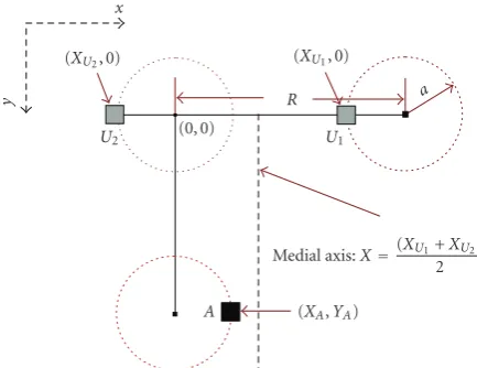
Figure5: Schematic of the node localization tolerance.
Figure 5shows the extreme instance of the node local-ization tolerance, where all sensor nodes are placed in the maximum tolerance positions. We calculate the maximum tolerance about the ideal and real scenario, respectively. The gray squaresU1andU2represent unknown nodes, and the black squareArepresents an anchor node. We suppose that the distance between nodes isR, and the tolerance of node localization is distancea.
In the absence of multipath fading and shadowing in ideal scenarios, RSSI distance measurement accurately represents the distance between any two sensor nodes. To avoid such equidistant instances in ideal scenarios, the bisector of two unknown abscissae (XU1+ XU2)/2 needs to
be larger than that of the abscissaXA of the nodeA. Their relation is expressed as follows:
(XU1+XU2)
2 > XA. (5)
Therefore, according to sensor nodes’ positions illus-trated in Figure 5, the above relation can be converted as follows:
(R−a−a)
2 > a. (6)
It is inferred that the localization tolerance should be less thanR/4, a quarter of the distance between any two sensor nodes in the grid topology about ideal scenarios.
In contrast to the ideal scenarios, RSSI distance measure-ment involves much error due to the presence of multipath fading and shadowing in the RF channel for real world. When the realistic precision of distance measurement based on RSSI is considered, the bisector of two unknown abscissae (XU1 +XU2)/2 needs to be larger than that of the abscissa
of the node A XA plus distance measurement error so as to distinguish neighboring nodes correctly. The tolerance relational expression should be revised as follows:
(XU1+XU2)
2 −XA> DP. (7)
DPrepresents the distance measurement error for a real world scenario. Consequently, the actual tolerance is given by
a < R
4−DP. (8)
To attain the correct position of a sensor node, the network must be carefully deployed within the scope of maximum tolerance which is given by subtracting the distance measurement error from a quarter of distance between sensor nodes.
4.4. Algorithm Simulation. In Kcdlocation, once the RSSI ranging technology can distinguish those neighboring unknown nodes relative to an anchor node within one hop, the algorithm will achieve the correct positions for sensor nodes. This requirement precision of ranging can be attained by many methods, even by RSSI in an environment of little disturbance. Therefore, the Kcdlocation provides relatively high localization precision under the low precision condition of ranging technology. As Kcdlocation and its assumptions are significantly different from the existing localization schemes, comparing the localization accuracy is not much meaningful.
To evaluate time and energy consumption of Kcdlocation algorithm, several simulations have been run on a square sensor network field. The network deployment approach is shown inFigure 1. In our scenario, the deployment nodes are arranged by a grid topology. Furthermore, we assume the use of an ideal medium access control (MAC). The MAC protocol is collision-free.
The time consumption for Kcdlocation is taken as a function of different network scales shown inFigure 6. For simplicity, the time for transmitting one frame is counted as a time unit. The time for localization of a node significantly depends on how far from anchors that node is, since the proposed localization algorithm executes in lock-step, with the nodes around an anchor localizing first and then extending to the whole network step by step.
The total number of frames, which are transmitted by all nodes during the process of localization under different network scales, is drawn inFigure 7.
According to Figures 6 and 7, the average time of localizing a node equals to that of transmitting 1.3 frames, and the average frames transmitted are 2.4 for localizing a node.
In addition, considering the fluctuation of real RSSI values, we use a filter to smooth the RSSI values. Usually averaging is the most basic filter method. The average RSSI value is simply calculated by transmitting a few packets from a node. Each time the RSSI value is measured and calculated according to the following equation:
RSSI= 1
N
i=N
i=0
RSSIi. (9)
0 200 400 600 800 1000 1200 1400
T
ime
co
nsumption,
Y
0 200 400 600 800 1000
Number of unknown nodes,X B
Figure6: Time consumption in Kcdlocation process.
and the average frames transmitted are 2.4∗Nfor localizing a node. By real experiments in different environments, the variable N is set to 10, which is enough to eliminate the fluctuation of RSSI values in most cases. To meet the actual application request in localization, a length of 15 bytes in each frame is enough.
As CC2420 chip is adopted in SKLTT node, developed by our lab, it provides an efficient data rate of 250 kps. The average time of localizing a node is 6.2 ms, and the average energy consumption per node in localization is about 1mJ when the node transmission power is set to 95 mW and the received power is set to 93 mW. This result is based on the power characterization of the SKLTT nodes [43].
Considering that many localization algorithms need to transmit hundreds of frames to exchange the information in the localization process, as compared to several frames transmitted in Kcdlocation, it can be deduced that the Kcdlo-cation algorithm own tremendous prepotency in localization time and energy consumption compared with many other localization algorithms.
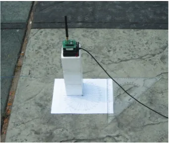
5. System Implementation and Evaluation
The Kcdlocation performances in a real system have been verified through two experiments, representing different RF channels and node deployments on SKLTT nodes shown in Figure 8.
SKLTT, a kind of wireless sensor network node with ultra low power consumption [43], was designed by our research group. Layer Division Multiplexing (LDM) is developed in SKLTT which uses C8051F121 microcontroller and CC2420 radio. The first experiment is conducted in a flat open area which represents an ideal obstruction-free RF channel, and the second experiment is conducted in our lab hall with no walls that represents RF channel under barrier condition.
As we have shown in our experiments as well as demon-strated in other research results [3, 4], radio irregularity is a common phenomenon in wireless sensor networks.
0 500 1000 1500 2000 2500
Tr
a
ffi
c
in
kc
d
location
pr
oc
ess,
Y
0 200 400 600 800 1000
Number of unknown nodes,X C
Figure7: Traffic in Kcdlocation process.
Figure8: SKLTT node onto a public square for the experimental placement.
Therefore, it is essential that we should take measures to decrease the effect of radio irregularity.
As shown in Figure 8, we select a 7 dBi omnidirectional high-performance antenna for SKLTT nodes and increase the height of radio antenna by using a foam supporter. We have adopted a standardized welding procedure for nodes fabrication, strictly selected all components with high consistency used in SKLTT nodes, and calibrated the radio for all the sensor nodes used in our experiments.
2
R
A1 R
√ 2R
Figure9: Schematic of node distinguishment process within one hop.
measurement in Kcdlocation are calculated as follows:
√
2R−R
R =
2R√−√2R
2R =41.4%. (10)
This means that the permissible distance measurement errors are up to 41.4% of the measured distance. So long as the precision of distance measurement using RSSI can distinguish between the grid distance and the diagonal grid distance, as well as the diagonal grid distance and the double grid distance, we will correct the grid locations for all unknown nodes by Kcdlocation algorithm.
After perfectly calibrating the radio characteristic in the real-test environments, the RSSI values are determined corresponding to different distances at a certain transmitting power level, such as grid distance, diagonal grid distance, and double grid distance, based on logarithmic curve fit between RSSI and range. Subsequently, two thresholds for the Kcdlocation system are set. The first threshold (RSSITH1)
is applied to distinguish nodes whether within one hop or not. The second threshold (RSSITH2) is used to judge which
node is nearer to anchor node and which node is farther to anchor node. The widely used signal propagation model is the log-normal shadowing model
RSSI(d)=PT−PL(d0)−10αln
d d0
+Xσ. (11)
Here,PTis the transmit power; PL(d0) is the path loss for a reference distanced0.αis the path loss exponent which is environment dependent.Xσ is a Gaussian random variable with zero mean, andσ2variance is modeled as the random
variation of the RSSI value. Thus, the distancedis the only variable in the equation. The Taylor series expansion method is used to analyze the variation of the ln(d) about a point
d=a
ln(d)=lna+d−a
a −
(d−a)2 2a2 +
(d−a)3 3a3
+· · ·+ (−1)n−1(d−a)n nan +Rn.
(12)
−70
−60
−50
−40
−30
−20
−10
RSSI,
Y
(dBm)
0 20 40 60 80 100 120
Range,X(ft)
Figure10: RSSI versus range in a flat open square.
−70
−60
−50
−40
−30
−20
−10
RSSI,
Y
(dBm)
−10 0 10 20 30 40 50 60 70
Range,X(ft)
Figure11: RSSI versus range in a building.
Considering the slight variation of RSSI value and the resource-constraint sensor nodes in these practical scenarios, one degree of the approximation polynomials in (12) can be fitted for the RSSI value, and the other higher order term can be omitted. For simplicity and practicality, the two thresholds are calculated as follows:
RSSITH1=
RSSI√2R+ RSSI2R
2 ,
RSSITH2=
RSSI√2R+ RSSIR
2 ,
(13)
where RSSIR, RSSI√2R, and RSSI2R are corresponding to the RSSI values measured at different subscript distances, respectively. The calibration parameters are stored in the MCU flash for subsequent judgment. In the implementation procedure of the Kcdlocation algorithm, only packets with an RSSI within the intervals are processed and judged. Packets with RSSI values not falling in the intervals are discarded.
Table1: Comparison of other location systems with Kcdlocation.
RADAR AHLoS Echolocation Probability Grid Kcdlocation
Need multianchor
nodes Yes, need multibase stations Yes Yes Yes
One anchor node
Hardware cost No extra component cost, but the location system is costly
High, combine ultrasound
module and RF to range Low Low Low
Computational cost High Low High High Low
Applicable to specific
topology No restriction No restriction Yes Yes Yes
Deployment
considerations RF signal mapping, Precalibration Precalibration Precalibration Precalibration Precalibration
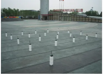
Figure12: Kcdlocation experimental scene at a park.
building with line of sight. From the figure, we can see that a perfectly logarithmic curve fits between RSSI and range in outdoor. However, the indoor-measured RSSI deviates significantly from the above logarithmic mode. This can be explained by multipath interferences in transmission media.
5.1. Outdoor Experiment. The first experiment is conducted in a flat open square located at Haidian Park in Beijing city, which represents a relatively obstruction-free RF channel, as shown inFigure 12.
The deployed system consists of 20 SKLTT nodes, all kept at a height of 1.2 ft above the ground, positioned in a 5∗4 grid, and grid distance is 5 ft. All the unknown nodes are deployed randomly on the grid positions, and an anchor node is placed in grid as well. One SKLTT sensor node is configured as a gateway, and it is attached to laptop through USB. Before implementing localization, the coordinate database of grids’ position placed by sensor nodes is inputted through localization visualization testbed shown in Figure 13, and then programmed to all deployed nodes over-the-air by virtue of gateway transmitting.
We use four vertex coordinates of network topology and grid distance to replace a coordinate database. The Kcdlocation algorithm is launched by the anchor node, and then gradually and orderly expands to all unknown nodes. After these unknown nodes have accomplished their localization processes, they transmit the position coordinates and the location time to the laptop through gateway and
display their positions on the localization visualization tool, shown in the left part ofFigure 13.
Figure 13 shows the position coordinates and the loca-tion time for all the unknown nodes after localizaloca-tion. The experimental results show that all the unknown nodes are located correctly. The average time of localizing a node is about 14.3 ms in the real implementation. The difference can be observed between the results produced in the simulator and the results obtained in the real-system implementation. The main cause for this difference is the use of an ideal medium-access control in the simulator, where the channel access is collision-free, and the use of the carrier sense multi-ple access with collision avoidance (CSMA-CA) mechanism for channel access in the real system, which adopts the random backoffand carrier sense to prevent collisions.
To derive the detailed procedure of Kcdlocation algo-rithm, we compare the location time of unknown node sequence number (ID) in implementation as shown in Figure 14. Actually, nodes with the same location time are localized in an identical atomic localization unit.
From the location time for different nodes, inFigure 15, the sequence of node location and the detailed procedure of node location are shown. The unknown nodesU1 andU2, which are nonequidistant with the anchor nodeAwithin one hop, were firstly located with the help of the anchor node
A, and then the procedure advances outwards sequentially to complete the whole network’s locations. The unknown nodes
U19andU20were localized in the tenth atomic localization unit ultimately. The whole location process needs 10 atomic localization units in total. The experiment results are in well agreement with the analysis of Kcdlocation algorithm.
U16 U17 U18 U19 U20
Figure13: The software interface of localization visualization.
0 Unknown node sequence number
Figure14: The location time of unknown node sequence number.
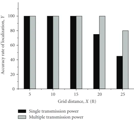
To improve the localization scalability of Kcdlocation, some measures have been taken in the algorithm imple-ment. First, considering that the multiple transmission power levels can cause a signal to propagate at various levels in its medium and show different characteristics at the receiver, the multiple transmission power levels are applied in localization that can be used to alleviate the effect of radio irregularity. The CC2420 supports 8
A
Figure15: The detailed procedure of node localization sequence.
discrete power levels. Before implementing localization, RSSI thresholds corresponding to different power levels are ascertained by radio calibration and then stored in MCU flash, which can be used to distinguish neighboring nodes.
0 20 40 60 80 100
A
ccur
acy
ra
te
of
localization,
Y
5 10 15 20 25
Grid distance,X(ft) Single transmission power Multiple transmission power
Figure 16: Localization accuracy comparison by using different transmission power.
eight coordinates is taken as the unknown node’s position. It is almost inevitable that there are some unknown nodes which have coordinates of the same highest frequency by coincidence. In this case, the unknown nodes can attain position messages of its neighboring nodes through pack-ets exchanging, and then assign the only grid coordinate that is not deployed to itself. If this method still fails to locate the unknown nodes, the mean of coordinates of the same highest frequency is taken as the unknown node’s position. Figure 16shows the benefits of the above improved method. It shows that the grid distance, where all unknown nodes can be localized correctly, increases to 20 ft.
Secondly, a method of multianchor nodes is adopted. As shown inFigure 17, four anchor nodes are placed at the four vertexes of network deployment and can launch the localization process from different directions and positions in turn. Consequently, each unknown node can locate its positions four times from diverse directions, and this can alleviate the effect of the nonisotropic RSSI and the randomness of environmental interference. Each unknown node has four coordinates as well. The coordinate occurring most frequently in the four coordinates is regarded as the unknown node’s position. If coordinates have the same frequency, we can adopt the same method used above to locate the unknown node.
Figure 18 shows the results of this improved method. The grid distance, where all unknown nodes can be located correctly, is up to 23 ft. This method increases the algo-rithm scalability significantly. However, using the improved method involves a trade-offin terms of higher time cost and energy consumption in the localization implement.
5.2. Indoor Experiment. The second experiment has been finished in the laboratory hall which represents the RF channel under a barrier condition. As shown in Figure 19,
the deployed system consists of 12 SKLTT nodes, positioned in a 3 ∗4 grid. The unknown nodes fail to locate their correct positions for most cases. It is suggested that nodes cannot distinguish their neighboring unknown nodes within one hop by using RSSI technology in a building because of the presence of multipath fading and shadowing in the RF channel. The experimental results show that the Kcdlocation algorithm has bad performance in the barrier condition. Being different from the outbuilding experiment, the environmental interference in a building is severe and intrinsic. Consequently, the improved methods applied in an outdoor experiment are not effective at improving those location estimates. Hence, for the Kcdlocation in a building, we can take other ranging schemes which have higher ranging precision than RSSI to improve location estimates, such as infrared, sound, and ultrasound [12– 17].
6. Comparisons with Other Location Systems
From the above experimental results, it can be concluded that the Kcdlocation algorithm achieves a localization performance with high precision, little time and energy consumption. As its presupposition is different from the localization qualifications of other algorithms, it is not meaningful to directly compare the localization precision with others. Therefore, our comparisons mainly focus on the number of anchor nodes to be needed, hardware cost, computational cost, applicability to network topol-ogy, and deployment considerations. To compare with Kcdlocation, we select four localization systems: RADAR [19], AHLoS [14], Echolocation [18], and Probability Grid [2], which are based on the criterion that they use RSSI during the localization process, and some of them have presuppositions that are similar to Kcdlocation. The four general solutions are described in the second section in more detail. Table 1 summarizes the compared results.
Compared with these four localization systems, the Kcd-location system only needs one anchor node to determine the coordinates of unknown nodes; moreover, it has a low hardware and computational cost. The algorithm is simple and has been shown to work fine in many test scenarios.
The Kcdlocation algorithm is applicable to all grid topologies, which means that in these scenarios the deploy-ment topology needs to adapt to the algorithm instead of other methods. This is just the same as the last two algo-rithms, Echolocation and Probability Grid. In addition, by using the RSSI technology to distinguish those neighboring nodes in the five localization systems, the precalibration of RSSI is an important step which should be adopted in the location system deployment; otherwise, a high location error will be produced.
U16 A3
A2
A1 C(4, 5)
C(−1, 4)
U17 U18 U19 U20
U6 U11
U1
A0 C(0, 4) T169.4 U12
C(1, 4) T169.4 U13
C(2, 4) T198
U14 C(3, 4) T278.3 U15
C(4, 4) T278.3
C(0, 3) T112.2 U7
C(1, 3) T112.2 U8
C(2, 3) T198
U9 C(3, 3) T253
U10 C(4, 3) T253
C(0, 2) T56.1
U2
C(0, 1) T28.6
C(0, 0) C(1, 1) T28.6
C(2, 1) T84.7 T140.8
C(3, 1) T225.5 C(4, 1) C(5, 1) C(1, 2)
T56.1 U3
C(2, 2) T84.7
U4 C(3, 2) T140.8 U5
C(4, 2) T225.5
R(0, 1)(4, 4)5
Figure17: Localization schematic diagram about multianchor nodes.
0 20 40 60 80 100
A
ccur
acy
ra
te
of
localization,
Y
5 10 15 20 25
Grid distance,X(ft) Single anchor node
Four anchor nodes
Figure 18: Localization accuracy comparison by using different anchor nodes.
7. Conclusions
We have presented an RF-based localization algorithm, which can be used in wireless sensor networks with a known coordinate database for exact network topologies, such as grid and linear types. Its performances of several real systems have been verified through different experiments,
Figure19: Experimental deployment for Kcdlocation in a building.
above qualification, we believe this requirement can be obtained in some sensor networks, and this localization algorithm can extend to other situations reliably. As this localization problem has not been considered before, a novel and practical localization algorithm is presented to satisfy the kind of sensor network deployment in the paper.
Acknowledgments
The paper is based on research funded through National Basic Research Program of China (973 Program) under project no. 2009CB320300, State 863 High Technology R&D key Project of China under Grant no. 2009AA045300, National key Technology R&D Program of China under Grant no. 2006BAD08B01, through NSFC under Grant no. 60773129, through the Excellent Youth Science and Technology Foundation of Anhui province of China under Grant no. 08040106808.
References
[1] I. F. Akyildiz, W. Su, Y. Sankarasubramaniam, and E. Cayirci, “Wireless sensor networks: a survey,”Computer Networks, vol. 38, no. 4, pp. 393–422, 2002.
[2] R. Stoleru and J. A. Stankovic, “Probability grid: a location estimation scheme for wireless sensor networks,” in Proceed-ings of the 1st Annual IEEE Communications Society Confer-ence on Sensor and Ad Hoc Communications and Networks (SECON ’04), pp. 430–438, October 2004.
[3] K. Whitehouse, C. Karlof, and D. Culler, “A practical evalua-tion of radio signal strength for ranging-based localizaevalua-tion,”
ACM SIGMOBILE Mobile Computing and Communications Review, vol. 11, no. 1, pp. 41–52, 2007.
[4] D. Lymberopoulos, Q. Lindsey, and A. Savvides, “An empirical characterization of radio signal strength variability in 3-D IEEE 802.15.4 networks using monopole antennas,” in
Proceedings of the 3rd European Workshop on Wireless Sensor Networks (EWSN ’06), vol. 3868 ofLecture Notes in Computer Science, pp. 326–341, Zurich, Switzerland, February 2006. [5] P. J. Marr ´on, M. Gauger, A. Lachenmann, D. Minder, O.
Saukh, and K. Rothermel, “FlexCup: a flexible and efficient code update mechanism for sensor networks,” inProceedings of the 3rd European Workshop on Wireless Sensor Networks (EWSN ’06), vol. 3868 ofLecture Notes in Computer Science, pp. 212–227, Zurich, Switzerland, February 2006.
[6] A. Arora, P. Dutta, S. Bapat et al., “A line in the sand: a wireless sensor network for target detection, classification, and tracking,” Computer Networks, vol. 46, no. 5, pp. 605–634, 2004.
[7] K. P. Ferentinos, T. A. Tsiligiridis, and K. G. Arvanitis, “Energy optimization of wireless sensor networks for environmental measurements,” inProceedings of the IEEE International Con-ference on Computational Intelligence for Measurement Systems and Applications (CIMSA ’05), pp. 250–255, July 2005. [8] L. B. Tik, C. T. Khuan, and S. Palaniappan, “Monitoring of
an aeroponic greenhouse with a sensor network,”International Journal of Computer Science and Network Security, vol. 40, no. 3, pp. 240–246, 2009.
[9] Z. Fang and Z. Zhao, “Some design issues of wireless sensor network for agriculture applications,” Tech. Rep., Institute of Electronics, Chinese Academy of Sciences, 2007.
[10] R. Stoleru, T. He, J. Stankovic, and D. Luebke, “A high-accuracy, low-cost localization system for wireless sensor networks,” in Proceedings of the 3rd ACM Conference on Embedded Networked Sensor Systems (SenSys ’05), pp. 250– 255, San Diego, Calif, USA, July 2005.
[11] S. Chen, Y. Chen, and W. Trappe, “Exploiting environmental properties for wireless localization and location aware appli-cations,” inProceedings of the 6th Annual IEEE International Conference on Pervasive Computing and Communications (PerCom ’08), pp. 90–99, March 2008.
[12] A. H. Sayed, A. Tarighat, and N. Khajehnouri, “Network-based wireless location: challenges faced in developing techniques for accurate wireless location information,” IEEE Signal Processing Magazine, vol. 22, no. 4, pp. 24–40, 2005.
[13] L. Girod and D. Estrin, “Robust range estimation using acoustic and multimodal sensing,” in Proceedings of the IEEE/RSJ International Conference on Intelligent Robots and Systems (IROS ’01), pp. 1312–1320, November 2001. [14] A. Savvides, C.-C. Han, and M. B. Strivastava, “Dynamic
fine-grained localization in ad-hoc networks of sensors,” in
Proceedings of the 7th Annual International Conference on Mobile Computing and Networking (MobiCom ’01), pp. 166– 179, July 2001.
[15] N. B. Priyantha, A. Chakraborty, and H. Balakrishnan, “Cricket location-support system,” inProceedings of the 6th Annual International Conference on Mobile Computing and Networking (MobiCom ’00), pp. 32–43, August 2000.
[16] J. Zhang, T. Yan, J. A. Stankovic, and S. H. Son, “Thunder: towards practical, zero cost acoustic localization for outdoor wireless sensor networks,”ACM SIGMOBILE Mobile Comput-ing and Communications Review, vol. 11, no. 1, pp. 15–28, 2007.
[17] D. Niculescu and B. Nath, “Ad hoc positioning system (APS) using AOA,” inProceedings of the 22nd Annual Joint Conference on the IEEE Computer and Communications Societies (INFO-COM ’03), pp. 1734–1743, April 2003.
[18] K. Yedavalli, B. Krishnamachari, S. Ravulat, and B. Srinivasan, “Ecolocation: a sequence based technique for RF localization in wireless sensor networks,” inProceedings of the 4th Interna-tional Symposium on Information Processing in Sensor Networks (IPSN ’05), pp. 285–292, April 2005.
[19] P. Bahl and V. N. Padmanabhan, “RADAR: an in-building RF-based user location and tracking system,” inProceedings of the 19th Annual Joint Conference of the IEEE Computer and Communications Societies (INFOCOM ’00), vol. 2, pp. 775– 784, March 2000.
[20] K. Lorincz and M. Welsh, “MoteTrack: a robust, decentralized approach to RF-based location tracking,” in Proceedings of the 1st International Workshop on Location- and Context-Awareness (LoCA ’05), pp. 63–82, Tel Aviv, Israel, May 2005. [21] L. M. Ni, Y. H. Liu, Y. C. Lau, and A. P. Patil, “LANDMARC:
indoor location sensing using active RFID,” in Proceedings of the 1st IEEE International Conference on Pervasive Com-puting and Communications (PerCom ’03), pp. 407–415, Fort Worth,Tex, USA, March 2003.
[24] P. Krishnan, A. S. Krishnakumar, W.-H. Ju, C. Mallows, and S. Ganu, “A system for LEASE: location estimation assisted by stationary emitters for indoor RF wireless networks,” in
Proceedings of the 23rd Annual Joint Conference of the IEEE Computer and Communications Societies (INFOCOM ’04), pp. 1001–1011, Hongkong, March 2004.
[25] A. M. Ladd, K. E. Bekris, A. Rudys, G. Marceau, L. E. Kavraki, and D. S. Wallach, “Robotics-based location sensing using wireless Ethernet,” in Proceedings of the 8th Annual International Conference on Mobile Computing and Networking (MobiCom ’02), pp. 227–238, September 2002.
[26] K. Kleisouris, Y. Chen, J. Yang, and R. P. Martin, “The impact of using multiple antennas on wireless localization,” inProceedings of the 5th Annual IEEE Communications Society Conference on Sensor, Mesh and Ad Hoc Communications and Networks (SECON ’08), pp. 55–63, June 2008.
[27] L. Doherty, K. S. J. Pister, and L. El Ghaoui, “Convex position estimation in wireless sensor networks,” in Proceedings of the 20th Annual Joint Conference of the IEEE Computer and Communications Societies (INFOCOM ’01), pp. 1655–1663, April 2001.
[28] Y. Shang, W. Ruml, Y. Zhang, and M. P. J. Fromherz, “Local-ization from mere connectivity,” inProceedings of the 4th ACM International Symposium on Mobile Ad Hoc Networking and Computing (MOBIHOC ’03), pp. 201–212, Annapolis, Md, USA, June 2003.
[29] Y. Shang and W. Ruml, “Improved MDS-based localization,” inProceedings of the 23rd Annual Joint Conference of the IEEE Computer and Communications Societies (INFOCOM ’04), pp. 2640–2651, Hongkong, March 2004.
[30] S. Lederer, Y. Wang, and J. Gao, “Connectivity-based local-ization of large scale sensor networks with complex shape,” in Proceedings of the 27th IEEE Communications Society Conference on Computer Communications (INFOCOM ’08), pp. 1463–1471, April 2008.
[31] Y. Wang, S. Lederer, and J. Gao, “Connectivity-based sensor network localization with incremental delaunay refinement method,” inProceedings of the 28th Conference on Computer Communications (INFOCOM ’09), pp. 2401–2409, April 2009. [32] N. Bulusu, J. Heidemann, and D. Estrin, “GPS-less low-cost outdoor localization for very small devices,” IEEE Personal Communications, vol. 7, no. 5, pp. 28–34, 2000.
[33] R. Nagpal, H. Shrobe, and J. Bachrach, “Organizing a global coordinate system from local information on an ad hoc sensor network,” inProceedings of the 8th International Conference on Information Processing in Sensor (IPSN ’03), vol. 2634 of
Lecture Notes in Computer Science, pp. 333–348, Palo Alto, Calif, USA, April 2003.
[34] M. Maroti, P. Volgyesi, S. Dora, et al., “Radio interferometric geolocation,” inProceedings of the 3rd International Conference on Embedded Networked Sensor Systems (SenSys ’05), pp. 1–12, San Diego, Calif, USA, November 2005.
[35] Y. Kwon, K. Mechitov, S. Sundresh, W. Kim, and G. Agha, “Resilient localization for sensor networks in outdoor envi-ronments,” in Proceedings of the 25th IEEE International Conference on Distributed Computing Systems (ICDCS ’05), pp. 643–652, June 2005.
[36] L. Fang, W. Du, and P. Ning, “A beacon-less location discovery scheme for wireless sensor networks,” in Proceedings of the 24th Annual Joint Conference of the IEEE Computer and Communications Societies (INFOCOM ’05), vol. 1, pp. 161– 171, Miami, Fla, USA, March 2005.
[37] W. Du, L. Fang, and P. Ning, “LAD: localization anomaly detection for wireless sensor networks,” inProceedings of the 19th IEEE International Parallel and Distributed Processing Symposium (IPDPS ’05), April 2005.
[38] T. He, C. Huang, B. M. Blum, J. A. Stankovic, and T. Abdelzaher, “Range-free localization schemes for large scale sensor networks,” in Proceedings of the 9th Annual Inter-national Conference on Mobile Computing and Networking (MobiCom ’03), pp. 81–95, September 2003.
[39] Z. Zhong and T. He, “MSP: multi-sequence positioning of wireless sensor nodes,” inProceedings of the 5th International Conference on Embedded Networked Sensor Systems (Sen-Sys ’07), pp. 15–28, Sydney, Australia, November 2007. [40] J. Jeong, S. Guo, T. He, and D. Du, “APL: autonomous passive
localization for wireless sensors deployed in road networks,” inProceedings of the 27th Annual Joint Conference of the IEEE Computer and Communications Societies (INFOCOM ’08), pp. 1256–1264, April 2008.
[41] R. Stoleru, P. Vicaire, T. He, and J. A. Stankovic, “StarDust: a flexible architecture for passive localization in wireless sensor networks,” inProceedings of the 4th International Conference on Embedded Networked Sensor Systems (SenSys ’06), pp. 57–70, November 2006.
[42] M. Li and Y. Liu, “Rendered path: range-free localization in anisotropic sensor networks with holes,” inProceedings of the 13th Annual International Conference on Mobile Computing and Networking (MobiCom ’07), pp. 51–62, Montreal, Canada, September 2007.