A Path Loss Model for Non Line of Sight Ultraviolet Multiple Scattering Channels

(1)

Volume 2010, Article ID 598572,12pages doi:10.1155/2010/598572

Research Article

A Path Loss Model for Non-Line-of-Sight Ultraviolet Multiple

Scattering Channels

Haipeng Ding,

1

_{Zhengyuan Xu,}

1

_{and Brian M. Sadler}

2

1_{Department of Electrical Engineering, University of California, Riverside, CA 92521, USA} 2_{Army Research Laboratory, RDRL-CIN, Adelphi, MD 20783, USA}

Correspondence should be addressed to Zhengyuan Xu,[email protected]

Received 1 December 2009; Accepted 30 March 2010

Academic Editor: Steve Hranilovic

Copyright © 2010 Haipeng Ding et al. This is an open access article distributed under the Creative Commons Attribution License, which permits unrestricted use, distribution, and reproduction in any medium, provided the original work is properly cited.

An ultraviolet (UV) signal transmission undergoes rich scattering and strong absorption by atmospheric particulates. We develop a path loss model for a Non-Line-of-Sight (NLOS) link. The model is built upon probability theory governing random migration of photons in free space, undergoing scattering, in terms of angular direction and distance. The model analytically captures the contributions of different scattering orders. Thus it relaxes the assumptions of single scattering theory and provides more realistic results. This allows us to assess the importance of high-order scattering, such as in a thick atmosphere environment, where short range NLOS UV communication is enhanced by hazy or foggy weather. By simulation, it is shown that the model coincides with a previously developed Monte Carlo model. Additional numerical examples are presented to demonstrate the effects of link geometry and atmospheric conditions. The results indicate the inherent tradeoffs in beamwidth, pointing angles, range, absorption, and scattering and so are valuable for NLOS communication system design.

1. Introduction

In free space optical communication, the deep ultraviolet (UV) spectrum with wavelength 200∼280 nm is regarded as an appealing choice to overcome solar background radiation and relax pointing and tracking [3]. High altitude ozone absorbs most solar radiation in this band, yielding negli-gible background noise at sea level [4]. And, atmospheric scattering is very strong, enabling non-line-of-sight (NLOS) communications where the transmitter is not necessarily within the receiver field of view (FOV). However, in addition to scattering, strong atmospheric absorption leads to significant signal attenuation and so limits achievable rates.

These properties have motivated development of UV signal propagation models and communication systems for military and civilian applications, for example, long-range communication based on high-power UV lasers since the 1960s [5–8]. Recent progress in deep UV light emitting diodes (LEDs) [9] and avalanche photo-diodes (APDs) [10, 11] oﬀers promise for deployment

of low-cost/power and moderate bandwidth short-range UV communication systems [12, 13], including underwa-ter communications [14, 15] and sensor networks [16,

17].

NLOS channel modeling is more complex than tra-ditional LOS links. In addition to wavelength and device characteristics, NLOS path loss is a function of system geom-etry, including transmitter (Tx) beamwidth, communication range, receiver (Rx) FOV, the pointing elevation angles, as well as the optical properties of the atmosphere.

(2)

the propagation distance is long. Alternatives to the single scattering model include an empirical path loss model [20] and a Monte Carlo statistical path loss model [2]. Those models are applicable for predicting path loss in a variety of scenarios and are generally more accurate than the single scattering model.

In this paper, following the same physical scattering law as the Monte Carlo statistical method [2, 21], we develop a stochastic analytical NLOS UV channel path loss model. We apply a stochastic analytical technique [22,23] to theoretically derive thenth scattered signal energy collected by the detector. The model assumes that the photons are stochastically scattered and/or absorbed by the atmospheric particles and involves probabilistic modeling of photon random moving direction, distance, energy loss, and receiver capture after a specified number of scatterings. In order to obtain thenth-order scattered signal at the receiver, we trace the migration routes of a single photon through the medium. Its scattering distance and scattering angles follow certain probability distribution functions (PDFs) [24]. The propagation of a photon between two consecutive scatterers is modeled as a single scattering event. The probability of the photon arriving at the receiver is a function of the

n scattering events encountered. A similar technique has been applied to model multiply scattered lidar returns in cloudy media where significant scattering occurs [22]. To account for a divergent UV beam profile, the contributions of photons at all possible directions within the beam are integrated [25].

We assume a homogeneous atmosphere with constant scattering and absorption coeﬃcients and ignore atmo-spheric turbulence. This assumes that diﬀerent types of particles are well mixed and the environment is stationary. Photons are scattered elastically which conserves energy but incurs energy loss during propagation. The detector is assumed small in size compared with the propagation space and is regarded as a point detector with finite FOV.

Our model offers an analytical formulation for NLOS scattering channel path loss and provides a reference to easily check other models in a variety of system parameter settings. We consider the effects of different optical pointing geometries and find that path loss is relatively insensitive to the Tx beam angle but increases considerably with increased Tx/Rx elevation angles and decreased Rx FOV for medium communication range. Not surprisingly, numerical tests demonstrate good agreement with Monte Carlo simulation [2]. However, the current analytical approach can distinguish the contributions of different orders of multiple scattering, whereas Monte Carlo modeling can only capture the total scattering effect. A similar comparison of Monte Carlo simulation and analytical methods has also been described by Lavigne et al. [26].

The model reveals when high-order scattering plays a role, and thus oﬀers more insight into the channel behavior. Extensive numerical tests show that high-order scattering may play a significant role for scenarios with large baseline ranges and elevation angles. Atmospheric conditions also aﬀect the multiple scattering contributions. A tenuous atmosphere generally leads to higher path loss at

β1 _β2

Figure 1: NLOS UV communication link geometry, depicting elevated transmitter beam and receiver field-of-view.

a small range than a thick or extra thick atmosphere where rich multiple scattering enhances received signal strength. As a by-product, when contributions from only single scattering are retained, the corresponding single scattering path loss shows a good match with that predicted by Reilly’s analytical single scattering model [1]. A disadvantage of the proposed model is that it cannot provide pulse spreading information, while the Monte Carlo model can [2].

The organization of this paper is as follows. The stochastic path loss model based on a general NLOS UV channel configuration is developed inSection 2. It consists of modeling photon direction, distance traveled, probability of arrival at the receiver after scatteringn times, and total path loss. Numerical analysis for the multiple scattering NLOS channel is carried out and path loss performance is compared with both the single scattering model and Monte Carlo simulation inSection 3. Channel characteristics under diﬀerent geometric parameters are analyzed in Section 4. Finally some conclusions are drawn.

2. Stochastic Path Loss Model

A NLOS UV channel involves rich scattering and absorption because of abundant suspended particulates in the atmo-sphere. For NLOS UV communication, scattering serves as the vehicle for information exchange between the Tx and Rx. The scattered photons that reach the receiver depend on the link geometry, the atmospheric optical properties, and their random migration, as described next.

2.1. Link Geometry. Consider a typical NLOS communica-tion geometry [19,20], as shown inFigure 1. Denote the Tx beam full-width divergence byα1, the Rx FOV angle byα2, the Tx elevation angle byβ1, Rx elevation angle byβ2, the Tx and Rx baseline separation byr, and the distances of the intersected (overlap) volumeV to the Tx and Rx byr1 and

r2, respectively.

(3)

the Rayleigh (molecular) scattering coeﬃcient ksRay, Mie (aerosol) scattering coeﬃcient kMie

s , absorption coeﬃcient

ka, and extinction coefficientke. The total scattering coeffi -cient is defined as the sum of the two scattering coefficients

ks = kRays + kMies , and the extinction coeﬃcient is given by the sum of the scattering and absorption coeﬃcients as

ke=ks+ka.

The scattering phase function is modeled as a combined function of Rayleigh and Mie scattering phase functions based on the corresponding scattering coeﬃcients [19,27]:

Pμ= k

whereμ =cosθis defined from the scattering angleθ. The two-phase functions follow a generalized Rayleigh model and a generalized Henyey-Greenstein function, respectively:

pRay_μ₌3

whereγ,g, and f are relevant model parameters.

2.3. Elementary Events for Photon Random Migration. Gener-ally, it is impossible to predict with certainty the trajectory of a photon that travels in a medium of randomly distributed scattering and absorption particles. However, based on single scattering theory, we can obtain the probabilities for a photon’s trajectory and calculate its multiple scattering arrival probability at the detector. The photon’s trajectory can be exactly described by scattering distance, scattering zenith angle θ, and scattering azimuth angle φ. We first present the PDFs of these three fundamental elements for our modeling. The distance between neighboring scatters can be modeled from sampling a uniform random variable

xbetween zero and one as r = −lnx/ks [28]. Accordingly after density transformation [29], the PDF of the scattering distancerbecomes

fr(r)=kse−ksr. (4)

The sample space for variable r is [0,∞]. The PDFs for zenith scattering angle θ and azimuth angle φ can be further formulated based on the scattering phase function. The zenith scattering angle under Rayleigh scattering, Mie

scattering, and combined Rayleigh and Mie scattering has the following PDFs:

where θ takes values in [0,π]. We consider a uniform distribution between 0 and 2π for azimuth scattering angle φ because there is no azimuth dependence in the phase function (symmetry is assumed). Thus, the azimuth scattering angle assumes the following PDF:

fφ

φ= 1

2π, φ∈[0, 2π]. (8)

2.4. Modeling ofnTimes Scattering. With those probabilities, we are able to develop a probability model for a photon to be received by the detector after exactly n scatterings. Assume that a photon from a UV source is uniformly emitted within the beam divergence and centered at direction angles θ0 and φ0, and migrates a distance r0 before the first scattering happens. The solid angle within the beam can thus be modeled as a uniform random variable with a constant PDF of 1/Ωs where Ωs is the source beam solid angle as Ωs = 2π(1−cos(α1/2)). The probability that it is scattered in the infinitesimal solid angle dΩ0 = sin(θ0)dθ0dφ0 becomes 1/Ωssin(θ0)dθ0dφ0 [22], and the probability that it moves an incremental distance dr0 with attenuation ise−kar0_f

r0(r0)dr0. Therefore the probability that

this photon lies away from the scatter center byr0and further movesdr0along the infinitesimal solid angle is the product of these two probabilities:

dQ0=e −kar0

Ωs fr0

(r0) sin(θ0)dθ0dφ0dr0. (9)

(4)

θ0

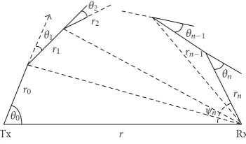
Figure2: Photon migration path fornscatterings.

all previous events can be written as

dQi=e−karifri(ri)fθi(θi)fφi

φi

sin(θi)dθidφidri. (10)

The same procedure can be successively applied for each scat-tering process. Assume that each scatscat-tering is self-governed, and the distances and angles for diﬀerent scattering events are conditioned on previous quantities. Therefore, the arrival probability for a photon that is scattered n times before arriving at the Rx can be derived based on these transitions.

Figure 2 shows the photon trajectory corresponding to n

scatterings.

After the nth scattering, we focus on an infinitesimal solid angle within the receiver FOV in order for the receiver to receive this photon. Define the direction angleψnas the angle between the line connecting the receiver and thenth scattering center and the transmitter-receiver separation line. Since the FOV has angle range of [β2 −α2/2,β2 + α2/2] as shown in Figure 1, we can confine the photon direction using an indicator function Inwhich equals one when the condition (β2−α2/2)< ψn<(β2+α2/2) is satisfied and zero otherwise. Therefore, the probability of the photon leaving thenth scattering center and reaching the detector becomes

dQn=Ine−kernfθn(θn)fφn

φn

sin(θn)dθndφn. (11)

We define the photon arrival probability afternscatterings asPn; that is, a photon undergoesnscatterings and arrives at the Rx. The photon trajectory is uniquely described by [(r0,. . .,rn), (θ0,. . .,θn), (φ0,. . .,φn)], which are scattering distance set, scattering zenith angle set, and scattering azimuth angle set for nsuccessive scatterings, respectively. These variables are associated with each other using distance vectors −→ri for i = 0,. . .,n, and all involved distances and scattering angles can be recursively obtained from the previous distance vectors [2,28]. Finally we obtain

Pn= · · ·

dQ0×dQ1· · · ×dQn, (12)

where dQ0 is given by (9), dQi by (10), and dQnby (11). The integration limits for all variables cover their full ranges except the following: θ0 from (β1 −α1/2) to (β1 + α1/2) to ensure integration inside the source beam, and θn and

φn within the solid angle of the receiver determined by the receiver area and distancern. Note that no integration over

rn is needed because it is a function of the other variables. Thus, there are a total of 3(n+ 1)−1 integration variables.

In our model, the arrival probability Pn is expressed through a multidimensional integral, and a closed form is not available. The dependence of rn and In on other variables creates additional diﬃculty in model evaluation, and asnincreases, the complexity increases. Hence we apply a Monte Carlo integration technique, a powerful but simple numerical integration method for the approximate evalua-tion of definite integrals [30]. The idea is to generate a large number of random sample points uniformly distributed in the multidimensional hypercube Dand then calculate the average value of the integrand from the random samples [22,30]. In our case we proceed as follows. There are (n+ 1) subspaces for 3(n+ 1)−1 integrals, represented by all thedQi. We randomly generate sample points for the first

n subspace integrations, and calculate the corresponding integrands from the generated sample points (ri,θi,φi) (i = 0, 1,. . .,n − 1), denoted by vector −→ri. We then obtain the location of the nth scattering center and calculate the quantity rn from all those sample values. Applying these results, we further calculate the index function In. If it is one, then we randomly generate a sample point for (θn,φn) and perform the integration over the detector area. This completes one sampling step. Suppose that the sample has a suﬃciently large sizeM, and denote the points in the sample by−→R1,. . .,−→RM. Then the estimate for the integral is given by

where for notational convenienceF(·) represents the inte-grand product of functions over all dQi, and d−→R for all differentialsd−→ri. During the process, we truncate the infinite integration limit for allri(up toi =n−1) at a sufficiently large number to ensure that the integrand has decayed sufficiently close to zero. We have found generally that using a limit of several times 1/ksworks well.

It is important to clarify the diﬀerence between the Monte Carlo integration of a definite integral as used here and the Monte Carlo simulation of a stochastic process [2]. Even though both belong to the Monte Carlo family and involve random realizations, Monte Carlo integration is a numerical method based on the approximation of the averaged deterministic integrand function, whereas Monte Carlo simulation is a technique that relies on repeated samplings (numerous realizations) of a random process to compute a statistical expectation.

2.5. Energy Loss Model. To obtain the NLOS channel energy loss, we assume that a UV source emits a pulse containing

N photons uniformly within the beam angle α1, and each photon has an energy . So the total transmitted energy is

Et = N. The received energy after n scatterings can be represented as

(5)

10−11 Figure3: Received energy ratio predicted by the proposed model.

Thenth scattering path loss is modeled as

PL(n)= Et

Er(n)= 1

Pn. (15)

The received total energy up tonscatterings is

Er,n=

From this result, the received energy ratio defined asEr,n/Et becomes ni=1Pi, and the corresponding path loss can be

Note that when n = ∞, the energy represents the total received energy contributed by all scatterings and path loss represents the actual link performance. If we adopt decibels for path loss, then it becomes 10 log₁₀(PLn).

3. Modeling Performance

(6)

80 85 90 95 100 105 110 115

P

ath

loss

(dB)

101 ₁₀2 ₁₀3

Range (m) (a) Path loss for (β1,β2)=(20◦, 20◦)

90 95 100 105 110 115 120 125

P

ath

loss

(dB)

101 ₁₀2 ₁₀3

Range (m) (b) Path loss for (β1,β2)=(45◦, 45◦)

90 100 110 120 130

P

ath

loss

(dB)

101 ₁₀2 ₁₀3

Range (m) n=1

n=2

n=1 n=3

Reilly (c) Path loss for (β1,β2)=(60◦, 60◦)

80 100 120 140 160

P

ath

loss

(dB)

101 ₁₀2 ₁₀3

Range (m) n=1

n=2

n=1 n=3

Reilly (d) Path loss for (β1,β2)=(90◦, 90◦) Figure4: Path losses predicted by the proposed model and Reilly’s model [1].

We assume gas concentrations and optical features of the atmosphere described by [7, Table II] for middle UV at wavelength 260 nm. Large dynamic ranges for the absorption and Mie scattering coefficients indicate that weather con-ditions may significantly affect the UV signal propagation. However, an explicit correspondence between the parameter settings and weather conditions is not available in the literature. Therefore we consider atmosphere coefficients for typical tenuous, thick, and extra thick atmosphere conditions (corresponding to clear, overcast, and foggy), given in

Table 1. The tenuous condition will be adopted for all the following results unless stated otherwise. This agrees with the experimental measurement conditions in [13]. We set the geometric and model parameters as follows: (α1,α2,β1,β2)

=(17◦, 30◦, 60◦, 60◦),r ranges from 10 m to 1000 m,γ = 0.017,g =0.72, f =0.5, and the detector area is 1.77 cm2_. Unless otherwise specified, the same parameters are used in

Section 4.

To illustrate the importance of multiple scattering, consider the following example. Figure 3 shows the ratio of the accumulated received energy from n = 1 (1st scattering order only) to n = 2 (sum of 1st and 2nd-order scatterings), and n = 3 (sum of 1st, 2nd and 3rd order scatterings), all predicted via our proposed stochastic modeling for diﬀerent optical geometries. We observe that, for each scenario, the 2nd-order scattering contributes little to the total received energy for ranges within 100 meters, but it will increasingly contribute more with longer ranges and larger pointing angles. Further, considering n = 3 does not add much to the received energy. For this case, 2nd-order scattering is suﬃcient because 3rd order scat-tering makes only a negligible contribution to the received energy.

The received signal energy can be transformed to the link path loss in decibels, depicted for diﬀerent geometries in

(7)

85 90 95 100 105 110 115 120

P

ath

loss

(dB)

101 ₁₀2 ₁₀3

90 100 110 120 130

P

ath

loss

(dB)

101 ₁₀2 ₁₀3

100 110 120 130

P

ath

loss

(dB)

101 ₁₀2 ₁₀3

Range (m) Stochastic

Simulation

(c) Path loss for (β1,β2)=(60◦, 60◦)

100 120 140 160

P

ath

loss

(dB)

101 ₁₀2 ₁₀3

Range (m) Stochastic

Simulation

(d) Path loss for (β1,β2)=(90◦, 90◦) Figure5: Comparison of the proposed stochastic model with the Monte Carlo simulation model [2].

single scattering model. Both models predict similar path loss levels forn = 1. As expected, including multiple scattering reduces predicted path loss. The improvement is not obvious for short range, consistent with Figure 3. Again, the 3rd-order scattering does not lead to a significant improvement for the received energy for these cases.

Due to the fact that our proposed stochastic model has the same premise that underlies the Monte Carlo simulation, we should expect the similar path loss from both models. As an example, Figure 5 compares the path loss results generated from our stochastic model and the Monte Carlo simulation model. Four sets of Tx and Rx elevation angles are included for detailed comparison. For each subplot, the stochastic model provides a good match with the simulation model within the high precision numerical accuracy of the simulation. This indicates that our proposed model is a good reference for evaluating the Monte Carlo simulation model.

4. NLOS UV Channel Characteristics

Since NLOS UV channel characteristics are crucial to communication system design, in this section, we apply the proposed multiple scattering model to further study the eﬀects of diﬀerent system parameters on the channel path loss, including link geometries and two typical atmosphere conditions. Referring toFigure 1, we study angle sensitivity by varying one angle and keeping the others fixed.

(8)

90 100 110 120 130

P

ath

loss

(dB)

101 ₁₀2 ₁₀3

Range (m) 20◦

60◦ 90◦

(a) Path loss for diﬀerentβ1

90 100 110 120 130

P

ath

loss

(dB)

101 ₁₀2 ₁₀3

Range (m) 20◦

60◦ 90◦

(b) Path loss for diﬀerentβ2

95 100 105 110 115 120 125 130

P

ath

loss

(dB)

101 ₁₀2 ₁₀3

Range (m) 17◦

30◦ 45◦

(c) Path loss for di_ﬀerentα1

90 100 110 120 130

P

ath

loss

(dB)

101 ₁₀2 ₁₀3

Range (m) 10◦

30◦ 45◦

(d) Path loss for di_ﬀerentα2 Figure6: Predicted path loss for diﬀerent system geometries.

range tends to make the angle effects more pronounced. As an example, in the first subplot for baseline range 1000 m, path losses for three different Tx elevation angles show differences up to 8 dB, while for a shorter range of 100 m, the difference is within 3 dB. Similar effects are obtained for other angular variation. One possible reason is that the roles of scattering and absorption may vary for different geometries. Larger propagation distance may bring about more scattered photons to the receiver but will also lead to higher absorption loss.

Up to now we have only considered tenuous atmospheric conditions. Next we consider the impact of atmospheric conditions on path loss. Figure 7depicts range-dependent path loss for tenuous, thick, and extra thick atmosphere

(9)

70 80 90 100 110 120 130

P

ath

loss

(dB)

101 ₁₀2 ₁₀3

80 90 100 110 120 130 140 150

P

ath

loss

(dB)

101 ₁₀2 ₁₀3

100 120 140 160

P

ath

loss

(dB)

101 ₁₀2 ₁₀3

Range (m) Tenuous

Thick Extra thick

(c) Path loss for (β1,β2)=(60◦, 60◦)

100 120 140 160 180

P

ath

loss

(dB)

101 ₁₀2 ₁₀3

Range (m) Tenuous

Thick Extra thick

(d) Path loss for (β1,β2)=(90◦, 90◦) Figure7: Predicted path loss for diﬀerent atmosphere conditions.

Table1: Atmosphere model parameters.

Atmosphere ksRay(km−1) ksMie(km−1) ka(km−1)

Tenuous 0.266 0.284 0.972

Thick 0.292 1.431 1.531

Extra thick 1.912 7.648 1.684

In these scenarios, the scattering contribution dominates absorption loss for short ranges. For larger baseline ranges, scattering loss increases as the atmosphere gradually becomes thick and thus causes large path loss. For a given atmospheric condition, path loss increases by 20 dB to 40 dB when the elevation angle increases from 20◦ to 90◦ at short range. These observations and predictions are helpful for experimental channel characterization and communication system design.

(10)

10−15 Figure8: Received energy ratio for extra thick atmosphere predicted by the proposed model.

yields significant high-order scattering contributions, such as 3rd- and 4th-order scatterings, which should be accounted for when predicting path loss. These results indicate the remarkable property that for relatively shorter ranges, NLOS UV communications links are enhanced in hazy or foggy weather.

5. Conclusions

This paper proposed an analytical energy loss model for NLOS UV communication channels based on the proba-bility theory of scattering and absorption. The model was developed by employing the PDFs of scattering distance and scattering angles. Multiple scattering was incorporated and contributions of diﬀerent scattering orders were identified. The total energy loss was modeled by summing over the

scattering order. The path loss predicted using only the con-tribution from the first-order agreed with Reilly’s analytical single scattering model, as illustrated with different optical geometries. Multiple scattering becomes more dominant for some cases, especially longer propagation distance and larger elevation angles. Our model also provided results that are consistent with the Monte Carlo simulation model. Channel characteristics were investigated in detail, including the effects of varying system geometry and the effects of different atmosphere conditions.

(11)

80 100 120 140

P

ath

loss

(dB)

101 ₁₀2 ₁₀3

80 100 120 140 160 180

P

ath

loss

(dB)

101 ₁₀2 ₁₀3

80 100 120 140 160 180 200

n=1 n=2 n=3

n=4 n=5

P

ath

loss

(dB)

101 ₁₀2 ₁₀3

Range (m)

(c) Path loss for (β1,β2)=(60◦, 60◦)

100 150 200 250 300 350 400

n=1 n=2 n=3

n=4 n=5

P

ath

loss

(dB)

101 ₁₀2 ₁₀3

Range (m)

(d) Path loss for (β1,β2)=(90◦, 90◦) Figure9: Predicted path loss for extra thick atmosphere.

Acknowledgments

The authors gratefully acknowledge R. Drost for his help with the coding examples. This work was supported in part by the U.S. Army Research Oﬃce under Grant W911NF-09-1-0293 and the Army Research Laboratory under the Collaborative Technology Alliance Program, Cooperative Agreement DAAD19-01-2-0011.

References

[1] D. M. Reilly and C. Warde, “Temporal characteristics of single-scatter radiation,”Journal of the Optical Society of America A, vol. 69, no. 3, pp. 464–470, 1979.

[2] H. Ding, G. Chen, A. K. Majumdar, B. M. Sadler, and Z. Xu, “Modeling of non-line-of-sight ultraviolet scattering channels for communication,”IEEE Journal on Selected Areas in Communications, vol. 27, no. 9, pp. 1535–1544, 2009.

[3] Z. Xu and B. M. Sadler, “Ultraviolet communications: poten-tial and state-of-the-art,”IEEE Communications Magazine, vol. 46, no. 5, pp. 67–73, 2008.

[4] L. R. Koller,Ultraviolet Radiation, John Wiley & Sons, New York, NY, USA, 2nd edition, 1965.

[5] G. L. Harvey, “A survey of ultraviolet communication sys-tems,” Tech. Rep., Naval Research Laboratory, Washington, DC, USA, March 1964.

[6] D. E. Sunstein, A scatter communication link at ultraviolet frequencies, B.S. thesis, MIT, Cambridge, Mass, USA, 1968. [7] D. M. Junge,Non-line-of-sight electro-optic laser

communica-tions in the middle ultraviolet, M.S. thesis, Naval Postgraduate School, Monterey, Calif, USA, December 1977.

[8] W. S. Ross and R. S. Kennedy, “An investigation of atmospheric optically scattered non-line-of-sight communication link,” type, Army Research Oﬃce Project Report, Research Triangle Park, NC, USA, January 1980.

(12)

quantum wells,”IEEE Journal on Selected Topics in Quantum Electronics, vol. 8, no. 2, pp. 302–309, 2002.

[10] X. Bai, D. Mcintosh, H. Liu, and J. C. Campbell, “Ultraviolet single photon detection with Geiger-mode 4H-SiC avalanche photodiodes,”IEEE Photonics Technology Letters, vol. 19, no. 22, pp. 1822–1824, 2007.

[11] S. C. Shen, Y. Zhang, D. Yoo, et al., “Performance of deep ultraviolet GaN avalanche photodiodes grown by MOCVD,”

IEEE Photonics Technology Letters, vol. 19, no. 21, pp. 1744– 1746, 2007.

[12] G. A. Shaw, A. M. Siegel, J. Model, and D. Greisokh, “Recent progress in short-range ultraviolet communication,” in Unattended Ground Sensor Technologies and Applications VII, Proceedings of SPIE, pp. 214–225, Orlando, Fla, USA, March 2005.

[13] G. Chen, F. Abou-Galala, Z. Xu, and B. M. Sadler, “Experimen-tal evaluation of LED-based solar blind NLOS communication links,”Optics Express, vol. 16, no. 19, pp. 15059–15068, 2008. [14] S. Arnon and D. Kedar, “Non-line-of-sight underwater optical

wireless communication network,” Journal of the Optical Society of America A, vol. 26, no. 3, pp. 530–539, 2009. [15] D. Kedard and S. Arnon, “Subsea ultraviolet solar-blind

broadband free-space optics communication,”Optical Engi-neering, vol. 48, no. 4, Article ID 046001, 7 pages, 2009. [16] G. A. Shaw, A. M. Siegel, J. Model, and M. Nischan, “Field

test-ing and evaluation of a solar-blind UV communication link for unattended ground sensors,” in Unattended/Unmanned Ground, Ocean, and Air Sensor Technologies and Applications VI, vol. 5417 ofProceedings of SPIE, pp. 250–261, Orlando, Fla, USA, April 2004.

[17] D. Kedar and S. Arnon, “Non-line-of-sight optical wireless sensor network operating in multiscattering channel,”Applied Optics, vol. 45, no. 33, pp. 8454–8461, 2006.

[18] M. R. Luettgen, J. H. Shapiro, and D. M. Reilly, “Non-line-of-sight single-scatter propagation model,”Journal of the Optical Society of America A, vol. 8, no. 12, pp. 1964–1972, 1991. [19] Z. Xu, H. Ding, B. M. Sadler, and G. Chen, “Analytical

performance study of solar blind non-line-of-sight ultraviolet short-range communication links,”Optics Letters, vol. 33, no. 16, pp. 1860–1862, 2008.

[20] G. Chen, Z. Xu, H. Ding, and B. M. Sadler, “Path loss modeling and performance trade-oﬀstudy for short-range non-line-of-sight ultraviolet communications,”Optics Express, vol. 17, no. 5, pp. 3929–3940, 2009.

[21] A. N. Witt, “Multiple scattering in reflection nebulae—I: a Monte Carlo approach,”The Astrophysical Journal Supplement Series, vol. 35, pp. 1–6, 1977.

[22] D. T. Gillespie, “Stochastic-analytic approach to the calcula-tion of multiply scattered lidar returns,”Journal of the Optical Society of America A, vol. 2, no. 8, pp. 1307–1324, 1985. [23] D. T. Gillespie, “Calculation of n-scattered lidar retrens for

large n in an idealized cloud,”Journal of the Optical Society of America A, vol. 4, no. 3, pp. 455–464, 1987.

[24] A. H. Gandjbakhche, R. Nossal, and R. F. Bonner, “Scaling relationships for theories of anisotropic random walks applied to tissue optics,”Applied Optics, vol. 32, no. 4, pp. 504–516, 1993.

[25] L. R. Bissonnette, “Multiple-scattering lidar equation,”Applied Optics, vol. 35, no. 33, pp. 6449–6465, 1996.

[26] C. Lavigne, A. Roblin, V. Outters, S. Langlois, T. Girasole, and C. Roz´e, “Comparison of iterative and Monte Carlo methods for calculation of the aureole about a point source in the Earth’s atmosphere,”Applied Optics, vol. 38, no. 30, pp. 6237– 6246, 1999.

[27] A. S. Zachor, “Aureole radiance field about a source in a scattering-absorbing medium,”Applied Optics, vol. 17, no. 12, pp. 1911–1922, 1978.

[28] S. A. Prahl, M. Keijzer, S. L. Jacques, and A. J. Welch, “A Monte Carlo model of light propagation in tissue,” in Dosimetry of Laser Radiation in Medicine and Biology, vol. IS 5 of

Proceedings of SPIE, pp. 102–111, 1989.

[29] A. Leon-Garcia,Probability and Random Processes for Electrical Engineering, Addison-Wesley, Reading, Mass, USA, 1994. [30] Wikipedia, “Monte Carlo integration,” http://en.wikipedia