R E S E A R C H
Open Access
A virtual queue-based back-pressure
scheduling algorithm for wireless sensor
networks
Zhenzhen Jiao
1, Baoxian Zhang
1, Wei Gong
1and Hussein Mouftah
2*Abstract
In this paper, we design a new virtual queue-based back-pressure scheduling algorithm (VBR) for achieving significant delay reduction in wireless sensor networks (WSN). Our algorithm design comes from an observation that classical back-pressure scheduling algorithm usually needs a long period of time to form a queue backlog-based gradient in a network, which decreases towards the sink in the network, before achieving stable packet delivery performance. To address this issue, VBR is designed to pre-build proper virtual queue-based gradient at nodes in a WSN, which is chosen to be a function of traffic arrival rate, link rate, and distance to sink, in order to be adaptive to different network and application environments while achieving high network performance. Moreover, the queue backlog differential between each pair of neighbor nodes is decided by their actual queue lengths and also their virtual queue lengths (gradient values). We prove that VBR can maintain back-pressure scheduling’s throughput optimality. Simulation result shows that VBR can obtain significant performance improvement in terms of packet delivery ratio, average end-to-end delay, and average queue length as compared with existing work.
Keywords: Back-pressure scheduling; Delay reduction; Wireless sensor networks
1 Introduction
Back-pressure algorithm has been considered as an efficient queue length-based scheduling and routing paradigm since its appearance [1]. It has attracted a lot of attention due to its remarkable advantages, e.g., through-put optimality (i.e., it can stabilize a network when the arrival rates lie within the capacity region of the net-work), achievable adaptive resource allocation, support to stateless and agile load-aware routing and scheduling, and simplicity. Recently, a lot of work (e.g., [2-21]) has been carried out, and much progress has been made to improve the performance of back-pressure scheduling in different network environments.
However, the poor delay performance of back-pressure algorithm is one of the key problems hindering its wide deployment in practice. To ease the understanding, in here, we briefly introduce how back-pressure schedul-ing works as follows. Back-pressure algorithm requires
*Correspondence: [email protected]
2School of Electrical Engineering and Computer Science, University of Ottawa, 800 King Edward Avenue, ON K1N 6N5 Ottawa, Canada
Full list of author information is available at the end of the article
each network node to maintain a queue for each flow traversing it (namely, per-flow queue). At each time slot, it works to activate (select) a set of non-interference links in the network (i.e., it selects a set of non-interference links for transmitting packets), which leads to the maxi-mum sum of link weights multiplying their corresponding link rates, to transmit packets. The link weight associated with a link is defined as the largest flow weight on the link, where the flow weight on a link is the queue back-log differential for the flow between the two endpoints of the link. However, such a scheduling strategy can often cause large latency, which is often attributed to the follow-ing three reasons. First, back-pressure-based schedulfollow-ing typically suffers from slow startup phenomenon. That is, when a flow starts, many packets of it have to be back-logged on the way to destination to form stable queue backlog-based gradient, which decreases towards the des-tination, for supporting smooth packet delivery to the destination. Such slow startup causes large initial end-to-end (E2E) packet delay. Second, fluctuation of the queue backlog-based gradient in the context of back-pressure
scheduling often causes data packets to take unneces-sarily long or even looped paths, which largely increases the packet delay. Third, the so-called last-packet prob-lem [13,14] can also cause large latency in networks with short-lived or low-rate flows due to the absence of consis-tent back-pressure towards the destination.
To address the above issues, in this paper, we design a virtual queue-based back-pressure routing and schedul-ing algorithm (called VBR) for wireless sensor networks (WSN). VBR is designed to pre-establish a virtual queue-based gradient for nodes in a WSN. In VBR, back-pressure-based scheduling is performed according to the queue length which is the sum of real queue length and virtual queue length (i.e., gradient value) at each node. The gradient associated with a node is a function of traffic arrival rate, network link rate, and its distance to sink, in order to be adaptive to different network and application environments while achieving high packet delivery per-formance. We prove that VBR maintains back-pressure’s throughput optimality. Simulation result shows that VBR can obtain significant performance improvement in terms of packet delivery ratio, average E2E delay, and average per-node queue length as compared with existing work.
The rest of the paper is organized as follows. Section 2 briefly reviews related work. Section 3 introduces the system model. Section 4 proposes the VBR algorithm. Section 5 presents detailed simulation results for perfor-mance comparison. Section 6 concludes this paper.
2 Related work
In this section, we briefly review related work for improv-ing delay performance of back-pressure schedulimprov-ing, which can be roughly divided into the following three categories based on their design objectives:
The first category aims at avoiding unnecessarily long or looped route which is often brought by back-pressure’s pure queue length differential-based scheduling strategy. For example, in [7], a routing-loop-punishment factor is introduced into the routing decision-making process. Similar idea but different factors can be seen in [6]. In [20,21], explicit hop constraint is used to force packets to be transmitted within a restricted area, with a worst-case deviation away from the min-hop path. Further, in [15], Ying et al. combined back-pressure scheduling and short-est path routing with an expectation to shorten the path length under back-pressure-based routing.
The second category is to reduce the complexity of queue structure at nodes. Typically, in [9,17], per-neighbor queue structure is used to replace the per-flow queue in classical back-pressure algorithm, which can significantly reduce the packet average delay. In [16], cluster-based back-pressure scheduling allows each node to maintain two types of queues, i.e., queues for gateways to reach destined cluster and queues for nodes within the
current cluster. In this way, it largely reduces the total number of queues needed to be maintained in the net-work. In [7], a last-in-first-out (LIFO) queue is used, which helps decrease the average packet delay.
The third category aims at relieving the last packet problem which often causes large latency in networks with dynamic short-lived or low-rate flows. For this pur-pose, the delay-based back-pressure scheduling in [14] assigns link weight based on packet delay instead of queue length differential. Ref. [13] proposes an adaptive redun-dancy technique for back-pressure routing, which gener-ates copies of packets to artificially increase the length of a queue when the queue’s occupancy is low, which dramat-ically improves the delay performance of back-pressure under light load condition. The idea in [13] is some-what similar to our work in this paper in terms of using artificially increasing the length of nodes’ queue lengths when calculating link weights. However, in [13], a packet’s duplicate copies in a queue need to be really transmit-ted. In contrast, the VBR algorithm in this paper only uses a virtual queue length (as a counter) for transmission scheduling decision-making and causes no extra packet to be transmitted.
It should be noted that the back-pressure-based routing and scheduling are quite different from the potential-based routing (gradient-potential-based routing) proposed in some previous work (e.g., [22,23]). Specifically, potential-based routing (gradient-based routing) jointly considers dis-tance to destination information (e.g., hop count), queue length information, residual energy of wireless nodes, etc., for route selection or next-hop decision-making. In potential-based routing, ideal potentials are expected to be constructed in a way such that paths taken by data packets are loop free. Data packets are usually forwarded to neighbors leading to the lowest (steepest) gradient. Such behavior, although attractive, may cause certain loss in network throughput. In contrast, in back-pressure-based routing, all the routing and scheduling decisions are made according to the queue length differences between the two ends of links in the network. Furthermore, when a packet can leave the current node where it stays and to which neighbor it will depart depends only on the ranks of the queue length differences between the two ends of the outgoing links of the current node in the entire net-work, which may change with time. Furthermore, in the context of back-pressure scheduling, there is no guaran-tee that paths taken by packets forwarded based only on back-pressure are loop free unless we pre-select loop-free paths for all flows and just use back-pressure algorithm for scheduling the packet transmissions on such paths.
3 System model
in the network, which consists of multiple sensor nodes and one sink node, andErepresents the set of links
con-necting the nodes in G. Each node is assumed to be
equipped with an omnidirectional antenna, and all nodes are assumed to have the same transmission range, denoted by R. A pair of nodes u andv,u,v ∈ V(G) has a link between them if dij ≤ R, where dij represents the geo-metrical distance betweenu andv. In VBR, no location information of nodes is assumed to be known. A WSN is often known as a converge-cast-based network, i.e., data packets can be generated by any sensor node and are reported to the sink node typically via multi-hop paths. In this paper, the packet arrival process is assumed to fol-low a Poisson process with arrival rate λ (packets/slot). It is known that back-pressure scheduling can always sta-bilize the network when the packet arrival rate is within the network capacity region. Here, the network capacity region is characterized by the maximum network sup-portable flow arrival rate vectors for which the network is stable (i.e., all queues in network are kept finite). In this paper, we focus on studying flows with arrival rates within the capacity region. Furthermore, from the viewpoint of the sink node in the network, data packets from all nodes can be seen as belonging to the same flow. This traffic modeling strategy has also been used in some other exist-ing work for WSNs (e.g., [7,20]). Assume time is slotted and is denoted byt. Accordingly, in such a network, the queue maintained by each node∈ V(G) for performing back-pressure-based scheduling and their queue dynam-ics are as follows. LetUnf(t)represent the per-flow queue backlog of the only flowf in the network on node n ∈ V(G)at timet. The dynamics ofUnf(t)at a nodenis as follows:
Unf(t+1) = max
Unf(t)−
bμ f nb(t), 0
+aμf
an(t)+Sfn(t), (1)
whereSfn(t)equals the number of packet(s) injected into the network vian if node n generates packet(s) at time t; otherwise, Sfn(t) = 0.μfab(t) represents the transmis-sion rate of flow f on link (a,b) at time t, and μfab(t) must satisfy the link rate constraint and also follow given link interference model. The interference model used in this paper is as follows. When a node is transmit-ting, all the links whose receivers are located within the transmitting node’s communication range will be seen as interfered. This model was also used in [24] (known as “unidirectional equal power” interference model therein). Furthermore, in this paper, we assume that all links in the network have the same link rate (capacity), denoted byr.
4 VBR algorithm
In this section, we first introduce the scheduling mech-anism in classical back-pressure algorithm. Then, we present the observation which motivates this work. Finally, we propose the algorithm design of VBR.
4.1 Classical back-pressure scheduling
The back-pressure scheduling algorithm was proposed in [1], and it works as follows. Assume time is slotted. At the beginning of a time slott, for each link(m,n)in the net-work, the weight associated with the link (i.e., link weight) is assigned as the maximum flow weight (i.e., the maxi-mum backlog differential of all the flows passing through the link, ties broken arbitrarily):
Wmn(t)=maxf:(m,n)
Umf (t)−Unf(t)
. (2)
Packets belonging to flowf will be transmitted over link
(m,n)if the link(m,n)is to be activated under a schedule
π(t), which is derived based on the following optimization function:
π(t)=arg maxπ∈(m,n)Wmn(t)r, (3)
whererepresents the set of all feasible schedules accord-ing to link interference model. Specially, since in this paper, we assume that all links have the same rates, and thus, the chosen schedule maximizes the sum of link weights among all schedules.
In back-pressure routing, when a packet leaves the cur-rent node where it stays and to which neighbor it will depart depends on the following: a) ranks of the queue length differences between the two ends of the outgoing links of the current node in the entire network; b) link rate; and c) whether there exists a link having been activated by the scheduling process in the interference range of a particular outgoing link. Moreover, all these factors may change with time (slots).
4.2 Motivation
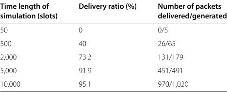
Before presenting our algorithm, let us first take a look at an example. Consider a linear network constituent of 50 nodes, which is to be traversed by a flow whose packet arrival follows a Poisson process with arrival rateλ= 0.1 and with the flow source and destination nodes as the two opposite end nodes of the network. The link rate of all links in the network is assumed to be one.
routing, the situation is different. To illustrate this, we per-form extensive simulations and Table 1 shows the results. In Table 1, it can be seen that the packet successful deliv-ery ratio under back-pressure routing increases with the simulation timea. The reason behind this phenomenon is as follows. The back-pressure algorithm always needs to form stable queue backlog-based gradient towards the destination to act as back-pressure for pushing packets forward, which is called slow startup phenomenon of back-pressure scheduling in this paper; otherwise, pack-ets may randomly walk in the network when no enough pressure is accumulated. As a result, when back-pressure algorithm starts to operate in a network, there is no enough time to build the destination-oriented gra-dient in the network, and thus, data packets can oscillate between (some) intermediate nodes since there is no con-sistent force to push them forward. As the network keeps operating, such destination-oriented queue length-based gradient will be gradually built, and the subsequent packet delivery process then comes stable (see Table 1). The forming of such destination-oriented queue length-based gradient needs many packets to stay on paths to the desti-nation, which can greatly increase the average-case packet delivery delay. Consequently, one question arises, whether such destination-oriented gradient can be pre-built before actual packet delivery and how it is useful (and also to which degree) for improving the network performance?
An intuitive way to solve the above question is to pre-establish certain gradient at nodes in a WSN. In this paper, we shall also treat such gradient associated with a sensor node as the virtual queue length at the sensor node. With-out causing confusion, we shall use the terms “gradient” and “virtual queue length” interchangeably unless other-wise stated. Accordingly, the queue backlog at a sensor node will be the sum of actual queue length and virtual queue length (gradient) at the node. LetQfmrepresent the gradient pre-built at a nodem ∈ V(G). Then, for a link
(m,n) ∈ E(G), the calculation of its link weight can be re-written into the following form:
Wmn(t)=maxf:(m,n)
Umf (t)+Qfm
−Unf(t)+Qfn
.
(4)
Table 1 Simulation results from a 50-node linear network
Time length of Delivery ratio (%) Number of packets simulation (slots) delivered/generated
50 0 0/5
500 40 26/65
2,000 73.2 131/179
5,000 91.9 451/491
10,000 95.1 970/1,020
Now, the question becomes how to appropriately set Qfm,∀m∈V(G), in order to achieve high network perfor-mance. In [25,26], the authors had also studied this issue, and they treated Qf as a shortest path bias such that its introduction is to force (actually encourage) data packets to take shortest paths. Accordingly, they suggested that Qf at a node should be proportional to its distance to the flow’s destination. More specifically, for a nodex∈V(G), its gradientQfxis calculated as follows.
Qfx=kHxf, (5)
whereHxf is the distance (e.g., hop count) from nodexto the destination of flowf andkis a constant. Whenk=1, the gradient at each node equals its hop count distance to the flow’s destination. In [25,26], the method in (4) and (5) for gradient establishment and link weight calcu-lation is called Enhanced Dynamic back-pressure Routing algorithm (EDR).
Although simple, the method for the gradient establish-ment in EDR has the following problems. First, it does not consider the dynamics in traffic arrival rate, which may change with time and applications. Setting a larger k can better force data packets to go through shortest paths. However, when traffic load is high, shortest paths may have insufficient transportation capacity. In this case,
using larger k can make EDR take much longer time
(as compared with classical back-pressure algorithm) to detour to alternate paths for packet delivery. In contrast, setting a smallerkmay result in frequent random walk of many data packets in the network, which could be even worse when the link rate (capacity) is high while the traf-fic load is moderate. Second, it uses constantkvalue (i.e., constant gradient slope) such that different distances away from the sink are equally treated without considering the traffic converging characteristics of a WSN. Under such a converging traffic pattern, in the region close to the sink node, transportation capacity is desired to be fully utilized; in contrast, in regions remote to the sink, fast packet delivery is desirable. Owning to these concerns, in this paper, we jointly consider link rate and path distance for appropriately setting the gradient at sensor nodes for achieving improved network performance.
4.3 Algorithm design and analysis
sink may take alternate paths due to the reduced gradient difference.
Based on the above considerations, in VBR, the gradient for a nodem∈V(G)is calculated as follows.
Qfm=a×bλ/H f
m×cHmf ×r, (6)
wherea,b, andcare network parameters and needed to be tuned via experiments. Next, we explain each compo-nent in (6) as follows:bλ/Hmf is an indicator for measuring the influence of packet arrival rate at a nodemwithHmf hop distance to sink. Here, the main reason that we divide the arrival rate by hop distance to sink is to increase the impact of arrival rate at nodes closer to the sink and especially increase the gradient difference between sink’s one-hop neighbor nodes and the sink itself, for which the reason is as follows, as we know, the vicinity of sink node in a WSN is often the bottleneck of the entire network. A large gradient difference between sink’s one-hop neighbor nodes and the sink itself can encourage sink’s neighbors to transmit to the sink so as to better use the limited capacity in sink’s neighborhood. The itemcHmf enables the gradi-ents at nodes increases exponentially with hop distance to sink. The itemris the link rate, and its introduction in (6) is to enable good adaptability to networks with different link rates. In addition, we have also tried many other func-tions for the virtual queue-based gradient calculation. The function given in (6) exhibits the best performance.
Next, we theoretically prove that VBR is throughput optimal as do classical back-pressure algorithm and also the EDR algorithm (proof for the latter can be found in [26]). Since our algorithm shares the same scheduling paradigm with EDR, i.e., (3) and (4), thus, the following lemma is given for proving the throughput optimality of VBR.
Lemma 1.Given finite constantand network size|V|, the virtual queue lengthQfm(∀m∈V(G))determined by VBR associated with pre-determined constant parameters a,b, andccan always be bounded byc|V|.
Proof.Recall thatQfm = a×bλ/H f
m ×cHfm×rin VBR.
Here,a,b, andcare constants.ris link capacity, and its value is always limited in realistic environments. Further-more, regarding bλ/Hmf , note thatbλ/Hmf ≤ bλ. Further, onlyλthat is within the network capacity region is con-sidered in the context of back-pressure scheduling. As a result, bλ ≤ ∞must hold. Thus, there always exists a finite constantthat makes the following equation holds, i.e., ≥ a×bλ/Hmf × r. Next, for the hop distanceHf
m frommto the sink, if a limited network size|V|is given, Hmf < |V|will hold (for simple networks as we study in this work). Thus, we can conclude thatQfm≤c|V|.
Next, it is known that the network is strongly stable if for each nodenand flowf the following equation can hold:
lim sup
In VBR, when virtual queue length is consid-ered, this condition changes to lim supt→∞1ttτ−=10E
Unf(τ)+Qfn
< ∞. However, under Lemma 1, we
can know that limn∈V(G)Qfn = O(|V|) holds for VBR. Thus, we can still prove the throughput optimality of VBR by using condition (7) and Lyapunov function
L(U) = n
Unf 2
as done in [26]. Specifically, since the queue dynamics in network at each time slot satisfy Unf(t + 1)≤max
Snf(t)(recall Equation (1)), consider the Lyapunov function
L(U) = nUnf 2
, where U(t) = Unf(t)n∈V(G), which denotes the vector process of backlog in each queue as a function of time. Next, the Lyapunov drift is then as follows: b2+2V(A−b)[8,26], we can have the following deduction:
Here, since there always exists a finite constant B
For this equation, since the arrival rates we con-sidered are below the network capacity region, thus,
there always exists a constant θ > 0 such that
Enaμfan(t)−bμ By substituting this into (13), we have:
(U(t))≤B−2
The time average of (15) yields:
lim sup
Thus, recall the condition (7), we can conclude that VBR can always stabilize the network when arrival rates lie within the capacity region of the network, i.e., it is throughput optimal.
5 Simulation results
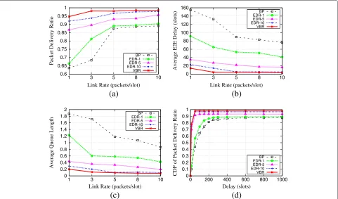
In this section, we evaluate the performance of VBR. We compare VBR with classical back-pressure algorithm (called BP for short) and EDR, on a random-generated network. Specifically, the network consists of 100 nodes randomly distributed within a 500×500 m2area, among which 99 nodes are sensor nodes and one is the sink, which is located close to the square center. The commu-nication range of all nodes is 100 m. In the network, the destination of all packets is the only sink node in the WSN. The packet arrival follows a Poisson process with arrival rateλ. For each packet generated, a random sensor node is picked as the packet source. In our simulations of VBR,
we chosea= 6,b =1.2, andc= 1.6, whose values were tuned via extensive simulations. We compared VBR with EDR with different values ofk, i.e.,k= 1, 5, and 10 (called EDR-1, EDR-5, and EDR-10, respectively). Via extensive simulations, we found that EDR can achieve its best
per-formance in most cases when k = 10. Each simulation
lasts 1,000 slots. The metrics used for performance eval-uation are packet delivery ratio, average E2E delay, and average queue length per node.
In our simulations, the commonly used greedy maximal scheduling (GMS) method was used for schedulable link set generation for each algorithm under comparison. This method is widely used for implementing back-pressure-based centralized algorithms under sophisticated net-works (e.g., [2,17,19]). When generating non-interference link schedule under GMS, at each time slot, a link(m,n) leading to the global maximum link weight is added to the link activation set, whose initial value is null. Further, remove the links which interfere with (m,n) and repeat the greedy selection until no link left. The GMS-based method can obtain schedule only with imperfect schedul-ing performance but has much lower computational com-plexity (i.e., O(|E|lg|E|) than the optimal solution whose complexity isO(|V|3)under one-hop interference model and in general NP-hard underK-hop interference mod-els (K ≥ 2) [27], where |E| is the number of links and |V|represents the number of nodes. Furthermore, it has been proven in [28] that the performance by GMS can achieve at least 1/2 of the optimal one for many net-work topologies and interference models, i.e., the capacity region supportable by GMS will be at least half of the opti-mal one. This result is further enhanced in [29] wherein the authors proven that in most networks, the scheduling performance under GMS is much better than the lower bound.
0.6
Average E2E Delay (slots)
Link Rate (packets/slot)
CDF of Packet Delivery Ratio
Delay (slots)
Figure 1Comparison of performance by different algorithms underλ=1.Link rate (packets/slot) versus(a)packet delivery ratio,(b)average E2E delay (slots),(c)average queue length, and(d)CDF of packet delivery ratio.
0.1
Average E2E Delay (slots)
Link Rate (packets/slot)
CDF of Packet Delivery Ratio
Delay (slots)
stablity of VBR. Figure 1d shows that cumulative distribu-tion funcdistribu-tion (CDF) of packet delivery ratio by different algorithms. We can see that VBR achieves the best CDF performance in terms of packet delivery ratio.
Figure 2 shows the simulation results versus link rates when λ = 5. From the results in Figure 2, we can see that as the link rate increases, the gap between VBR and the other two algorithms increases. One key reason for this is because VBR considers link rate in gradient setting while EDR does not. The results in Figure 2 again ver-ify the superiority of VBR by pre-establishing appropriate gradient at nodes in a network.
We have also repeated our simulations on linear net-works consisting of 30 to 50 nodes, a 4 × 4 mesh grid network, and other random networks. Similar results were observed. Thus, we can conclude that VBR outperforms EDR and BP in terms of packet delivery ratio, average E2E delay, and average queue length under various network scenarios.
6 Conclusions
In this paper, we proposed a new virtual queue-based back-pressure scheduling algorithm VBR, which pre-establishes gradient at each node in a WSN and inte-grates this gradient when calculating the queue back-log differential between neighboring nodes when making back-pressure-based scheduling decision. We proved the throughput optimality of VBR. Simulation results show that VBR can significantly improve network performance in terms of packet delivery ratio, average E2E delay, and average queue length at each node as compared with existing work.
Endnote
aIn Table 1, when the simulation comes to the 50thslot,
the packet delivery ratio performance is 0%. We repeated this test multiple times, and the same result was always seen. However, in practice, the probability of having a packet to reach the destination at the 50thslot based on our network settings is not zero (although extremely low). For example, suppose at the 50thslot, only one packet was generated, then the probability for the packet to reach the destination will be(1/2)49based on the back-pressure based scheduling in (3).
Competing interests
The authors declare that they have no competing interests.
Acknowledgements
This work was supported in part by the National Natural Science Foundation of China under Grant Nos. 61101133, 61471339, 61173158.
Author details
1Research Center of Ubiquitous Sensor Networks, University of Chinese
Academy of Sciences, No.19A Yuquan Road, 100049 Beijing, China.2School of Electrical Engineering and Computer Science, University of Ottawa, 800 King Edward Avenue, ON K1N 6N5 Ottawa, Canada.
Received: 11 May 2014 Accepted: 15 January 2015
References
1. L Tassiulas, A Ephremides, Stability properties of constrained queueing systems and scheduling policies for maximum throughput in multihop radio networks. IEEE Trans. Autom. Control.37, 1936–1948 (1992) 2. X Lin, N Shroff, inCDC’04: Proceedings of 43rd IEEE Conference on Decision
and Control. Joint rate control and scheduling in multihop wireless networks (IEEE, Atlantis, BAHAMAS, 2004), pp. 1484–1489 3. A Eryilmaz, R Srikant, inINFOCOM’05: Proceedings of 24th Annual Joint
Conference of the IEEE Computer and Communications Societies. Fair resource allocation in wireless networks using queue-length based scheduling and congestion control (IEEE Miami, FL, 2005), pp. 1794–1803 4. MJ Neely, E Modiano, C Li, inINFOCOM’05: Proceedings of 24th Annual Joint Conference of the IEEE Computer and Communications Societies. Fairness and optimal stochastic control for heterogeneous networks (IEEE, Miami, FL, 2005), pp. 1723–1734
5. MJ Neely, R Urgaonkar, Optimal backpressure routing for wireless networks with multireceiver diversity. Ad Hoc Netw.7, 862–881 (2009) 6. A Dvir, AV Vasilakos, inSIGCOMM’10: Proceedings of the ACM SIGCOMM
2010 Conference. Backpressure-based routing protocol for DTNs (ACM, New Delhi, INDIA, 2010), pp. 405–406
7. S Moeller, A Sridharan, B Krishnamachari, O Gnawali, inIPSN’10: Proceedings of the 9th ACM/IEEE International Conference on Information Processing in Sensor Networks. Routing without routes: the backpressure collection protocol (ACM/IEEE, Stockholm, SWEDEN, 2010), pp. 279–290 8. H Seferoglu, E Modiano, inINFOCOM’13: Proceedings of 32th Annual Joint Conference of the IEEE Computer and Communications Societies. Diff-max: Separation of routing and scheduling in backpressure-based wireless networks (IEEE, Turin, ITALY, 2013), pp. 1555–1563
9. L Bui, R Srikant, AL Stolyar, A novel architecture for reduction of delay and queueing structure complexity in the backpressure algorithm. IEEE/ACM Trans. on Netw.19, 1597–1609 (2011)
10. A Warrier, S Janakiraman, S Ha, I Rhee, inINFOCOM’09: Proceedings of 28th Annual Joint Conference of the IEEE Computer and Communications Societies. DiffQ: practical differential backlog congestion control for wireless networks (IEEE, Rio de Janeiro, BRAZIL, 2009), pp. 262–270 11. B Radunovic, C Gkantsidis, D Gunawardena, P Key, inMobiCom’08:
Proceedings of the 14th ACM International Conference on Mobile Computing and Networking. Horizon: balancing TCP over multiple paths in wireless mesh network (ACM, San Francisco, CA, 2008), pp. 247–258
12. R Laufer, T Salonidis, H Lundgren, PL Guyadec, inMobiCom’11: Proceedings of the 17th ACM International Conference on Mobile Computing and Networking. Xpress: A cross-layer backpressure architecture for wireless multi-hop networks (ACM, Las Vegas, NV, 2011), pp. 49–60
13. M Alresaini, M Sathiamoorthy, B Krishnamachari, MJ Neely, in INFOCOM’12: Proceedings of 31th Annual Joint Conference of the IEEE Computer and Communications Societies. Backpressure with adaptive redundancy (BWAR) (IEEE, Orlando, FL, 2012), pp. 2300–2308 14. B Ji, C Joo, NB Shroff, inINFOCOM’11: Proceedings of 30th Annual Joint
Conference of the IEEE Computer and Communications Societies. Delay-based back-pressure scheduling in multi-hop wireless networks (IEEE, Shanghai, CHINA, 2011), pp. 2579–2587
15. L Ying, S Shakkottai, A Reddy, S Liu, On combining shortest-path and back-pressure routing over multihop wireless networks. IEEE/ACM Trans. on Netw.19, 841–854 (2011)
16. L Ying, R Srikant, D Towsley, S Liu, Cluster-based back-pressure routing algorithm. IEEE/ACM Trans. on Netw.19, 1773–1786 (2011)
17. E Athanasopoulou, L Bui, T Ji, R Srikant, A Stolyar, Back-pressure-based packet-by-packet adaptive routing in communication networks. IEEE/ACM Trans. on Netw.21, 244–257 (2013)
18. B Ji, C Joo, NB Shroff, inINFOCOM’13: Proceedings of 32th Annual Joint Conference of the IEEE Computer and Communications Societies. Exploring the inefficiency and instability of back-pressure algorithms (IEEE, Turin, ITALY, 2013), pp. 1528–1536
19. Z Jiao, Z Yao, B Zhang, C Li, inICC’13: Proceedings of IEEE International Conference on Communications. Nbp: An efficient network-coding based backpressure algorithm (IEEE, Budapest, HUNGARY, 2013), pp. 1625–1629 20. Z Jiao, Z Yao, B Zhang, C Li, inICC’14: Proceedings of IEEE International
anycast-based back-pressure framework for wireless sensor networks (IEEE, Sydney, AUSTRALIA, 2014), pp. 2815–2820
21. L Maglaras, D Katsaros, inWoWMoM’11: Proceedings of IEEE International Symposium on a World of Wireless, Mobile and Multimedia Networks. Layered back-pressure scheduling for delay reduction in ad hoc networks (IEEE, Lucca, ITALY, 2011), pp. 1–9
22. A Basu, A Lin, S Ramanathan, inSIGCOMM’03: Proceedings of the 2003 Conference on Applications, Technologies, Architectures, and Protocols for Computer Communications. Routing using potentials: a dynamic traffic-aware routing algorithm (ACM, Karlsruhe, GERMANY, 2003), pp. 37–48
23. D Kominami, M Sugano, M Murata, T Hatauchi, inMSWiM’11: Proceedings of the 14th ACM International Conference on Modeling, Analysis and Simulation of Wireless and Mobile Systems. Controlled potential-based routing for large-scale wireless sensor networks (ACM, Miami, FL, 2011), pp. 187–196 24. P Chaporkar, K Kar, X Luo, S Sarkar, Throughput guarantees in maximal
scheduling in wireless networks. IEEE Trans. on Inf. theory.54, 572–594 (2008)
25. MJ Neely, E Modiano, C Rohrs, Dynamic power allocation and routing for time varying wireless networks. IEEE J Sel. Areas Commun.23, 89–103 (2005)
26. L Georgiadis, MJ Neely, L Tassiulas,Resource Allocation and Cross-layer Control in Wireless Networks. (Now Publishers Inc, Boston, 2006) 27. G Sharma, NB Shroff, R Mazumdar, inMobiCom’06: Proceedings of the 12th
ACM International Conference on Mobile Computing and Networking. On the complexity of scheduling in wireless networks (ACM Los Angeles, CA, 2006), pp. 227–238
28. X Lin, NB Shroff, The impact of imperfect scheduling on cross-layer congestion control in wireless networks. IEEE/ACM Trans. on Netw.14, 302–315 (2006)
29. C Joo, NB Shroff, inINFOCOM’07: Proceedings of 26th Annual Joint Conference of the IEEE Computer and Communications Societies.
Performance of random access scheduling schemes in multi-hop wireless networks (IEEE, Anchorage, AK, 2007), pp. 1481–1493
Submit your manuscript to a
journal and benefi t from:
7 Convenient online submission
7 Rigorous peer review
7 Immediate publication on acceptance
7 Open access: articles freely available online
7 High visibility within the fi eld
7 Retaining the copyright to your article