Combining earthquake forecasts using differential probability gains

F U L L P A P E R

Open Access

Combining earthquake forecasts using

differential probability gains

Peter N Shebalin

, Clément Narteau

, Jeremy Douglas Zechar

and Matthias Holschneider

Abstract

We describe an iterative method to combine seismicity forecasts. With this method, we produce the next generation of a starting forecast by incorporating predictive skill from one or more input forecasts. For a single iteration, we use the differential probability gain of an input forecast relative to the starting forecast. At each point in space and time, the rate in the next-generation forecast is the product of the starting rate and the local differential probability gain. The main advantage of this method is that it can produce high forecast rates using all types of numerical forecast models, even those that are not rate-based. Naturally, a limitation of this method is that the input forecast must have some information not already contained in the starting forecast. We illustrate this method using the Every Earthquake a Precursor According to Scale (EEPAS) and Early Aftershocks Statistics (EAST) models, which are currently being evaluated at the US testing center of the Collaboratory for the Study of Earthquake Predictability. During a testing period from July 2009 to December 2011 (with 19 target earthquakes), the combined model we produce has better predictive performance - in terms of Molchan diagrams and likelihood - than the starting model (EEPAS) and the input model (EAST). Many of the target earthquakes occur in regions where the combined model has high forecast rates. Most importantly, the rates in these regions are substantially higher than if we had simply averaged the models.

Keywords: Probabilistic forecasting; Earthquake interaction; Forecasting and prediction; Statistical seismology

Background

Despite a growing number of reasonably reliable and skillful numerical seismicity forecast models, operational earthquake forecasting remains a daunting challenge. One of the fundamental difficulties is that operational fore-casts require high expected earthquake rates to make substantial decisions (e.g., evacuation or other emergency actions), but the probabilities derived from statistical seis-micity models are still quite small (Jordan and Jones 2010). One potential approach to this problem is to combine models in a way that maximizes overall predictive skill.

It is well known that combining many models or clas-sifiers that describe the same data may yield higher per-formances than any individual member. These ensemble learning techniques include methods such as Bayesian

*Correspondence: [email protected]

1Institute of Earthquake Prediction Theory and Mathematical Geophysics, 84/32 Profsouznaya, Moscow 117997 Russia

2Equipe de Dynamique des Fluides Géologiques, Institut de Physique du Globe de Paris, Sorbonne Paris Cité, Univ Paris Diderot, UMR 7154 CNRS, 1 rue Jussieu, Paris 75238, France

Full list of author information is available at the end of the article

model averaging (Marzocchi et al. 2012) and, in the con-text of classifiers, boosting (Hastie et al. 2008). In the first case, the combined model is a weighted sum of individual posterior probabilities, the weights being new parameters that can be learned from the data. For boosting, weighted data are used to train a collection of classifiers; during iteration, previously misclassified data get higher weight. These approaches are similar in that the combined mod-els or classifiers are of the same abstract nature, meaning that each gives a statistical description of the same data set. In our approach, we combine models of different natures. For example, alarm-based and rate-based fore-cast models both give a description of the seismicity in a region. However, alarm-based models do this through a space-time alarm function, generally not normalized, whereas rate-based models give a description in terms of space-time Poisson event rates. The combination of two such models cannot be cast into the classical form used in ensemble techniques. Furthermore, the vast majority of current seismicity models are based only on catalogs of past earthquakes, and there is some hope that addi-tional geological, geodetic, and physical information could

improve forecast performance. Combining such informa-tion should be done in a complementary fashion so as not to increase uncertainty and thereby degrade forecast performance. This challenge cannot be met by tradi-tional methods, and a new method to combine forecasts should identify what additional information a model can contribute to an existing forecast.

It is often difficult to verify the presence of additional predictive information in an earthquake forecast model, but researchers are attempting to address this prob-lem with the Collaboratory for the Study of Earthquake Predictability (CSEP). In CSEP testing regions around the world (e.g., California, Italy, New Zealand, the western Pacific, Japan, and the globe), various forecast mod-els are evaluated in a standardized way (Jordan 2006; Gerstenberger et al. 2007; Zechar et al. 2010a; Zechar and Jordan 2010; Zechar et al. 2010b; Rhoades and Gerstenberger 2009; Nanjo et al. 2011; Tsuruoka et al. 2012; Eberhard et al. 2012; Taroni et al. 2014). One sub-tle benefit of these centers is that all forecasts are sys-tematically archived. Therefore, one can test methods of combination using archived prospective forecasts. Most forecasts within CSEP testing centers are rate-based fore-cast models with a time step of 1 day, 3 months, or 5 years, and testing regions are gridded with square cells of 0.1◦ and a class interval of earthquake magnitude of 0.1 from

M≥3.95 earthquakes. For a much longer period, several alarm-based models have been developed and tested by various research groups. Known examples are the global and regional tests of M8, CN, and RTP (Keilis-Borok and Kossobokov 1990; Keilis-Borok and Rotwain 1990; Peresan et al. 1999; Shebalin et al. 2006; Romashkova and Kossobokov 2004; Zechar 2010).

Researchers have suggested a few methods for combin-ing models and/or earthquake precursors. For a set of rate-based models, a weighted average is a natural solu-tion (Rhoades and Gerstenberger 2009; Marzocchi et al. 2012; Rhoades 2013). In the current implementation of such approaches weights do not depend on space; rather, they are chosen according to a relative performance of the model observed during some testing period. A direct product of functions describing precursory behavior was used in the RTL prediction algorithm (Sobolev et al. 1996). In this case, even if the initial functions are probabilis-tic, the output is a nonprobabilistic alarm-based model. Another way to combine models is by using Bayes’ for-mula for conditional probabilities (Sobolev et al. 1991). However, when using this approach, it is difficult to take into account the interdependence of the combined ele-ments, and resulting estimates are hardly probabilistic.

Shebalin et al. (2011) suggested a method based on differential probability gains to convert alarm-based to rate-based earthquake forecast models. Thus, nonprob-abilistic forecast models or seismic precursor maps can

be converted to probabilistic rate-based models. In this article, we generalize this differential probability gains approach to combine all types of time-varying forecasts.

Methods

Evaluation of forecast models

Following the CSEP standards, we discretized forecasts in space and time according to a predefined grid and a given time step. In prospective tests, all forecasts are given for the next time step and a finite magnitude range.

Molchan tests

Molchan tests are used to compare an alarm-based model with a reference model of seismicity defined on the same spatial grid (Molchan 1990). For any space-time region (x,t), the reference model provides the rate λ(x,t) of target earthquakes. The alarm-based model is entirely defined by its alarm function A(x,t). Where this alarm function exceeds a given threshold value A0, an alarm is issued and a target earthquake is expected to occur. Although it is not necessary, it is usually assumed thatA

values are ordered from smallest to largest according to the probability of occurrence of a target event. In almost all cases, numerical forecast models can be easily con-verted to an alarm-based forecast because the information provided by a numerical value assignment on a given space-time grid can be used as an alarm function.

A Molchan test takes the form of a diagram comparing rates of types I and II errors for varying threshold values

A0 (i.e., a level of alarm). For differentA0 values, type I

errors are measured by

τ (A0)=

A(x,t)≥A0

λ(x,t)

λ(x,t) , (1)

where the sum symbols refer to the space-time regions in which the subscript condition is satisfied. Theτ value is often interpreted as a fraction of the space-time region occupied by alarms (Kossobokov and Shebalin 2003; Molchan 2010). Here, it is important to emphasize that this fraction is given by a reference model that may depend on time. Type II error rates are the miss ratesν(A0), the fraction of target earthquakes that occurred in space-time bins in whichA<A0.

In a Molchan diagram, the(τ,ν)curve constructed for all A0 values is called the Molchan trajectory (Molchan

1990; Zechar and Jordan 2008). This trajectory runs from the point (0, 1) to the point (1, 0) for a decreasing A0

The closer the Molchan trajectory is to the y axis, the more skill the forecast has. It is often desirable to char-acterize forecast skills by a scalar value, the so-called loss function. Examples of loss functions are the mini-mal summary error (Molchan 1990, max(1−τ−ν)), the minimax loss function (Molchan 1990, inf(max(ν, τ ))), the area above the Molchan curve (Zechar and Jordan 2008; 2010), and the maximal probability gain (Aki 1996, max((1 − ν)/τ )). If there are a large number of target events, we can also suggest here the target-weighted prob-ability gain (i.e., max((1−ν)2/τ )). Note the singularity at τ = 0 for many of these expressions. Furthermore, there is always a trade-off between the rates of false alarms and failures to predict so that the best scalar value may depend on the goal of the forecast (Molchan 1990). In all cases, one should plot the two-dimensional Molchan diagram to visualize the vector data that are processed.

Likelihood tests

Likelihood tests are commonly used to evaluate rate-based models of seismicity. Their forecasts are tested against the numberω(x,t)of observed target earthquakes in each bin (Schorlemmer et al. 2007). For simplicity, indi-vidual rates are assumed to follow independent Poisson processes. For all magnitude classes, the complete like-lihood counts the Poisson joint log-likelike-lihood of the observed numberω(x,t)given the forecastλ(x,t):

L(t)=(−λ(x,t)+ω(x,t)log(λ(x,t))−log(ω(x,t)!).

(2)

The closer the joint log-likelihood is to zero, the better the forecast is.

The spatial likelihood is a reduction of the complete likelihood applied to a forecast with rate value normalized to match the total observed number of targets (Zechar et al. 2010a). In each spatial bin, the single rate values are obtained by summing the expected event rates over the whole range of magnitudes (Kossobokov 2006). For the total duration of the experiment, the total sum of log like-lihoods over all time steps can be calculated and divided by the total number of observed events to estimate a log likelihood per earthquake.

Likelihood tests applied to forecasts defined on a high-density spatial grid are often criticized because of poten-tial earthquake interactions (Molchan 2012). However, the problem of bin independence cannot be solved easily and it is generally thought that the dependence is condi-tional on earthquake occurrence. For example, we expect many aftershocks after large earthquakes, but a prospec-tive forecast experiment requires any interbin dependence

to be provided in advance, before one knows about the large earthquake (Zechar 2010).

Testing forecast models at CSEP

Likelihood and Molchan tests are complementary and both can be used to estimate the performance of the fore-cast models. The likelihood tests, however, do not apply to nonprobabilistic alarm-based models.

At CSEP testing centers, all the rate-based models are evaluated by using likelihood tests. In contrast, alarm-based models are only tested at the California testing center using Molchan tests and the related ROC and ASS tests (Zechar and Jordan 2008; Zechar 2010). Unfor-tunately, alarm- and rate-based models are still tested independently. The main reason for this is that the like-lihood tests cannot be applied to an alarm-based model with a nonprobabilistic alarm function. To address this problem, Shebalin et al. (2012) proposed a method to convert alarm-based models to rate-based forecasts. In addition, two rate-based models can be compared by using Molchan diagrams. In practice, the complete rate-based model should be reduced to a single rate value by summing over a given range of magnitude. The reduced model can be treated as a rate-based model and/or as an alarm-based model. Its alarm function is sim-ply composed of the single rate value in each spatial cell.

In summary, all requirements are satisfied for system-atic implementation of both likelihood and Molchan tests. The next challenge is to identify the regions of particu-lar skill for each model and combine models in a way that increases the expected event rates.

A differential probability gain approach for combining two earthquake forecast models

Here, we generalize the concept of differential probabil-ity gain to combine different types of earthquake fore-cast models. The main idea is to successively create new generations of a rate-based model by injecting into the current generation the additional information provided by other input models. In what follows, we describe one iteration of the combination procedure using a current model (the initial rate-based forecast model at the first iteration) and an input model (any type of numerical forecast model) to compute a new rate-based forecast model.

In a Molchan diagram, we can define the probability

whereA0is the threshold value of the alarm function, and

the sum symbols refer to the space-time regions in which the subscript condition is satisfied. ThisGvalue is a fac-tor that integrates the increase of the rate of the current model within the space-time region in whichA>A0(Aki 1981; Molchan 1991; Zechar and Jordan 2008). To iso-late smaller areas and specific behaviors associated with different ranges of the alarm function, we work with the differential probability gain function that can be defined as the derivative of a continuous Molchan trajectory,

g_inputcurrent= −∂ν/∂τ. (4)

With the small samples we have in practice, the Molchan trajectory is always a steplike function. We smooth this function using a limited number of segments to avoid overfitting the differential probability gain function (see Appendix 1). Finally, for each segment and the corre-sponding range [A0;A0+δA0] of alarm function values,

we have a differential probability gain of

g_inputcurrent= − ν/ τ=

where the sum is taken over to the space-time regions in which the subscript condition is satisfied. Considering all segments, we can assign a specific g_inputcurrent value to any

A value of the input model. Having done that, we can produce space-time maps of the differential probability gain of the input model and combine them with the cur-rent rate-based model. Then, the next generation of the rate-based model is defined as

λ_new=g_inputcurrent(A(x,t))λ_current, (6)

that is, the initial rates of the current model increase or decrease according to the local g_inputcurrent value. The

g_inputcurrent values are always estimated retrospectively over long times to be used in future applications.

This method of model combination is similar to con-volving the current model with the input model. For this reason, in the following, we denote one iteration of this procedure by

new model = (current model)∗(input model).

Results and discussion

Combining Every Earthquake a Precursor According to Scale and Early Aftershocks Statistics forecast models in California

The Every Earthquake a Precursor According to Scale (EEPAS) and Early Aftershocks Statistics (EAST) models are forecast models installed at the CSEP Testing Center in California. They are of special interest for this study because, based upon the joint evaluation using Molchan tests outside the official CSEP testing process, it was found that they both yield statistically significant better forecasts than a Relative Intensity (RI) reference model, a time-independent model that is commonly used as a reference model in Molchan tests (Kossobokov and Shebalin 2003; Helmstetter et al. 2006; Molchan and Keilis–Borok 2008; Zechar and Jordan 2008).

The EEPAS model (Rhoades and Evison 2004; 2007) is a medium-term forecast model based on the precur-sory scale increase phenomenon and associated predic-tive scaling relations (Evison and Rhoades 2004). In this model, every earthquake is a precursor according to scale, with the scale referring to larger earthquakes to follow in the medium to long term. Then, smaller earthquakes are ‘witnesses’ of the seismogenic process and not ‘actors’ as in the well-known branching model ETAS (Ogata 1989). Several versions of the EEPAS model have been used to generate forecasts of seismicity for the next 3 months. They have been tested at the California CSEP testing cen-ter since January 2008. Among the five versions of this forecast model, we chose the EEPAS-0F model (hence-forth referred to as simply the EEPAS model) because it performs the best against the RI reference model.

The EAST model is an alarm-based earthquake fore-cast model that uses early aftershock statistics (Shebalin et al. 2011). This model is based on the hypothesis that the time delay before the onset of the power-law aftershock decay rate decreases as the level of stress, and the seismo-genic potential increase (Narteau et al. 2002; 2005; 2008; Narteau et al. 2009). In contrast to the EEPAS model, the EAST model is not a model of seismicity rates. Instead, it possesses a nonprobabilistic alarm function that is dedi-cated to detecting places with a higher level of stress where an earthquake is more likely to occur. These zones are identified by relatively low values of the geometric mean of elapsed times between mainshocks and early aftershocks. The three-month class EAST model has been archived at the California CSEP center since July 2009.

To perform all the likelihood tests for CSEP testing centers, a rate-based version of the EAST model has been developed by Shebalin et al. (2012). Here, this new rate-based model called EASTR can be described as a

the initial alarm-based model, its forecast skill is likely to depend on the conversion method. This is also true for the combining method developed here, especially since it can be applied to two time-dependent models.

In all our tests, we consider two testing regions: the offi-cial CSEP California testing region and a subset, with the idea that the subset will reduce the problem of reduced earthquake detectability in the ocean and outside the USA (Shebalin et al. 2011). We also consider a retrospective period from January 1984 to June 2009 and a quasi-prospective time period from July 2009 to December 2011. The official CSEP test started on 1 July 1 2009, for the EAST model and earlier for the EEPAS model, and all model parameters for EEPAS, EAST, and gEEPAS_EAST were fixed beforehand. Note that to set up the EAST model and to calculate the functionsg_EASTEEPAS, we only use the testing region subset.

Cross-evaluation of earthquake forecast models

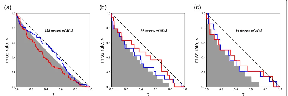
To underline how different forecast models may pro-vide independent information about seismicity, we per-form a cross-evaluation of the EASTRand EEPAS models

using Molchan diagrams (Figure 1). In both retrospec-tive (Figure 1a) and quasi-prospecretrospec-tive tests (Figure 1b,c), Molchan trajectories are below the diagonal, indicating that each model provides a gain in prediction with respect to the other (see Subsection ‘Molchan tests’). Although at first glance these results might appear contradictory, we interpret this as an indication that the EASTRand EEPAS

models are complementary. Because they focus on differ-ent relevant aspects of seismicity, each of them gives an additional amount of predictive information.

This complementary nature of two independent mod-els of seismicity is difficult to detect using likelihood tests (Table 1). However, we stress the point that it may be an important property for earthquake forecasting and cer-tainly the best case to combine two independent models. Then, the method to combine must preserve the knowl-edge gain that each model offers.

Here, we use the differential probability gain method to combine two forecast models. We infer that the increase in expected rates may be locally high, particularly if sev-eral models are successively combined. For one iteration, the combination is driven by the slope of the Molchan tra-jectories. Therefore, it is ideal to have two models that are substantially complementary in their forecasts. As shown by Figure 1, this condition is satisfied by the EAST and EEPAS models, and their combination may yield new predictive information on California seismicity.

A combination of EAST and EEPAS forecast models using differential probability gains

As shown by (Shebalin et al. 2012), there is no significant difference in the predictive power of the EAST and EASTR

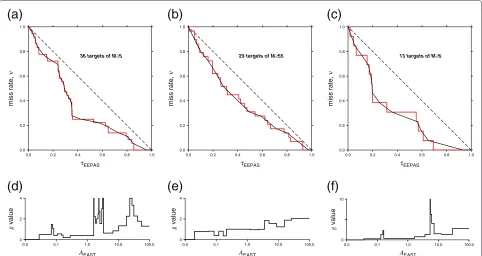
models. Therefore, to avoid potential noise introduced by the RI reference model or the conversion method, we combine directly the EAST and EEPAS models. To con-struct the differential probability gain functionsgEEPAS_EAST, we consider the retrospective period and three magnitude ranges of [4.95; 5.45), [5.45; 5.95), and [5.95;∞). Within each of those intervals, the combined model inherits the magnitude distribution of the EEPAS model, which is not constrained to follow the Gutenberg-Richter relation in each cell. Figure 2 shows for each interval the Molchan

(a) (b) (c)

0.0 0.2 0.4 0.6 0.8 1.0

miss rate,

ν

0.0 0.2 0.4 0.6 0.8 1.0

τ 128 targets of M≥5

0.0 0.2 0.4 0.6 0.8 1.0

miss rate,

ν

0.0 0.2 0.4 0.6 0.8 1.0

τ 19 targets of M≥5

0.0 0.2 0.4 0.6 0.8 1.0

miss rate,

ν

0.0 0.2 0.4 0.6 0.8 1.0

τ 14 targets of M≥5

Figure 1Cross-evaluation of the EEPAS and EASTRmodels in California forM≥4.95 target earthquakes.(a)Retrospective period from

January 1984 to June 2009.(b and c)Quasi-prospective period from July 2009 to December 2011. We consider the entire CSEP testing region in (b)and a reduced region in(a)and(c)to exclude off-coast and outside USA areas (Shebalin et al. 2011). Using Molchan diagrams, we compare the forecasts of the EASTRmodel with respect to the EEPAS model (red lines) andvice versa(blue lines). The dashed diagonal line corresponds to an

unskilled forecast. The shaded area indicates the zone in which the prediction of the tested model outperforms the prediction of the reference model at a level of significanceα=1%. For both the EEPAS and the EASTRmodels, we consider single rate values obtained by summing the

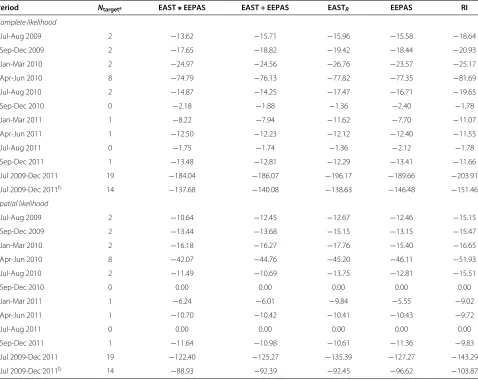
Table 1 Complete and spatial likelihood results for the forecasts

Period Ntargeta EAST∗EEPAS EAST + EEPAS EAST_R EEPAS RI

Complete likelihood

Jul-Aug 2009 2 −13.62 −15.71 −15.96 −15.58 −18.64

Sep-Dec 2009 2 −17.65 −18.82 −19.42 −18.44 −20.93

Jan-Mar 2010 2 −24.97 −24.56 −26.76 −23.57 −25.17

Apr-Jun 2010 8 −74.79 −76.13 −77.82 −77.35 −81.69

Jul-Aug 2010 2 −14.87 −14.25 −17.47 −16.71 −19.65

Sep-Dec 2010 0 −2.18 −1.88 −1.36 −2.40 −1.78

Jan-Mar 2011 1 ₋8.22 ₋7.94 ₋11.62 ₋7.70 ₋11.07

Apr-Jun 2011 1 ₋12.50 ₋12.23 ₋12.12 ₋12.40 ₋11.55

Jul-Aug 2011 0 ₋1.75 ₋1.74 ₋1.36 ₋2.12 ₋1.78

Sep-Dec 2011 1 −13.48 −12.81 −12.29 −13.41 −11.66

Jul 2009-Dec 2011 19 −184.04 −186.07 −196.17 −189.66 −203.91

Jul 2009-Dec 2011b _{14 −137.68 −140.08 −138.63 −146.48 −151.46}

Spatial likelihood

Jul-Aug 2009 2 −10.64 −12.45 −12.67 −12.46 −15.15

Sep-Dec 2009 2 −13.44 −13.68 −15.15 −13.15 −15.47

Jan-Mar 2010 2 −16.18 −16.27 −17.76 −15.40 −16.65

Apr-Jun 2010 8 −42.07 −44.76 −45.20 −46.11 −51.93

Jul-Aug 2010 2 −11.49 −10.69 −13.75 −12.81 −15.51

Sep-Dec 2010 0 0.00 0.00 0.00 0.00 0.00

Jan-Mar 2011 1 ₋6.24 ₋6.01 ₋9.84 ₋5.55 ₋9.02

Apr-Jun 2011 1 ₋10.70 ₋10.42 ₋10.41 ₋10.43 ₋9.72

Jul-Aug 2011 0 0.00 0.00 0.00 0.00 0.00

Sep-Dec 2011 1 ₋11.64 ₋10.98 ₋10.61 ₋11.36 ₋9.83

Jul 2009-Dec 2011 19 −122.40 −125.27 −135.39 −127.27 −143.29

Jul 2009-Dec 2011b _{14 −88.93 −92.39 −92.45 −96.62 −103.87}

a_N

targetis the number ofM≥4.95 earthquakes during the indicated periods.

b_{Reduced region to exclude off-coast and outside USA areas. Complete and spatial likelihood results for the forecasts of the EAST∗EEPAS, linear combination}

EAST+EEPAS (half and half), EASTR, EEPAS, and RI reference models.

diagrams, their approximation by segments, and the dif-ferential probability gain functions of the EAST model with respect to the EEPAS model. We observe that the

g_EASTEEPAS values are greater than one for almost two orders of magnitude of the alarm function of the EAST forecast model (Figure 2d,e,f ).

For three magnitude intervals we use the corresponding functionsgEEPAS

EAST and the ratesλEEPAS of the EEPAS model

in Equation 6 to obtain the rates of the new rate-based model EAST∗EEPAS. Figure 3 shows Molchan diagrams used to evaluate the forecast of the EAST, EEPAS, and EAST∗EEPAS models with respect to the RI reference model during the quasi-prospective period. The compar-ison of these Molchan trajectories shows that the com-bined model works better than the two initial models from which it has been derived. This is particularly the case for the smallest τRI value, for which both initial models

perform better than the RI reference model at a signif-icance level below α = 1%. Results of total likelihood and spatial likelihood (Table 1) indicate also a gain of the EAST∗EEPAS model with respect to the EEPAS model. Quantitatively, the log-likelihood gain is 0.30 and 0.26 per earthquake for total and spatial likelihoods, respectively. With respect to the EASTRmodel, these gains are 0.34 and

0.43, respectively.

(a)

(b)

(c)

0.0 0.2 0.4 0.6 0.8 1.0

miss rate,

ν

0.0 0.2 0.4 0.6 0.8 1.0

τEEPAS

0.0 0.2 0.4 0.6 0.8 1.0

miss rate,

ν

0.0 0.2 0.4 0.6 0.8 1.0

τEEPAS

0.0 0.2 0.4 0.6 0.8 1.0

miss rate,

ν

0.0 0.2 0.4 0.6 0.8 1.0

τEEPAS 36 targets of M≥5 29 targets of M≥55 13 targets of M≥6

(d)

(e)

(f)

0 2 4

g

value

0.0 0.1 1.0 10.0 100.0

AEAST

0 2 4

g

value

0.0 0.1 1.0 10.0 100.0

AEAST

0 10

g

value

0.0 0.1 1.0 10.0 100.0

AEAST

Figure 2Differential probability gain functions for EAST model with respect to EEPAS model.Estimation of the differential probability gain functions,gEEPAS

EAST, of the EAST forecast model with respect to the EEPAS model for California from January 1984 to June 2009.(a, b, and c)Molchan

diagrams, in which we smooth the Molchan trajectory (red line) by a set of segments (black lines; see Appendix 1). ThegEEPAS

EAST value is the local slope

of these segments.(d, e, and f)Differential probability gaingEEPAS

EAST as a function of the alarm functionAEASTof the EAST models. We use three

nonoverlapping magnitude intervals of [ 4.95; 5.45)in(a)and(d), [ 5.45; 5.95)in(b)and(e), and [5.95;∞)in(c)and(f). Note that for(a)and(d), we use a shorter time period from January 1995 to June 2009 to eliminate aftershocks of the Landers earthquake.

(a) (b)

0.0 0.2 0.4 0.6 0.8 1.0

miss rate,

ν

0.0 0.2 0.4 0.6 0.8 1.0

τRI

0.0 0.2 0.4 0.6 0.8 1.0

miss rate,

ν

0.0 0.2 0.4 0.6 0.8 1.0

τRI

19 targets of M≥5 14 targets of M≥5

Figure 3Quasi-prospective evaluation of the EAST∗EEPAS, EASTR, and EEPAS models.Quasi-prospective evaluation (July 2009 to December

2011) of the EAST∗EEPAS, EASTR, and EEPAS models with respect to the RI reference model in California. Tests were done in the entire California

CSEP testing region(a)and in a reduced region(b)that does not include off-coast and outside USA areas (Shebalin et al. 2011). Using Molchan diagrams, we compare the forecasts of the EAST∗EEPAS (black lines), EASTR(red lines), and EEPAS (blue dashed lines) models with respect to the RI

is smaller, 0.05 for total likelihood and 0.25 for spatial likelihood.

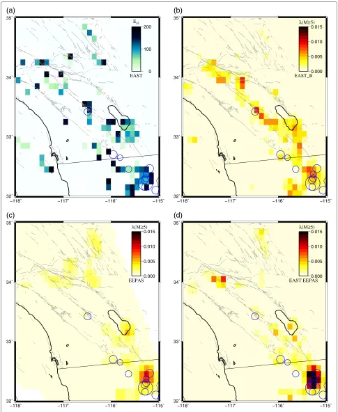
Figure 4 illustrates how our combining method works using the outputs of the EAST, EASTR, EEPAS, and

EAST∗EEPAS models for the forecast period from April to June 2010 along the USA-Mexico border. This space-time region includes theM7.2 El Mayor-Cucapah earth-quake of 4 April 2010. Figure 4a shows the map of the EAST alarm function values. For rate-base models (Figure 4b,c,d), the rates are calculated for M ≥ 4.95 events by summation of all model rates in correspond-ing magnitude bins. All models exhibit a clear maximum near the epicenter of the El Mayor-Cucapah earthquake. However, in an area extending northward from this epi-center, the EAST∗EEPAS model gives rates that are almost one order of magnitude larger than the rates of the two individual models. This example demonstrates that our combining method sharpens these individual forecasts, providing higher expected earthquake rates in more con-fined areas. These local increases of the forecast event rates are compensated by decreases in other places so that the total event rate over the whole territory does not significantly change (see Appendix 2).

Comparing combining methods

Using the weighted average of two rate-based models is straightforward and therefore the most common combin-ing method (Rhoades and Gerstenberger 2009; Marzocchi et al. 2012) . In addition, the use of weighted averages may increase the total predictive skill of the resulting model by locally giving more importance to high and low extreme rate values of each model. However, it remains an averaging method. Then, if the combined model keeps the total expected earthquake rate (convex combina-tion) unchanged, local rates cannot be higher (or lower) than the maximum (minimum) rates of the two mod-els. One exception is the combination of models that concentrate on forecasting different seismic patterns (for example, so-called mainshocks and aftershocks (Rhoades and Gerstenberger 2009)). In that case, it is not neces-sary to keep the total rate unchanged, and the combined rates may exceed the maximum of the two models being combined.

Here, we compare the EAST∗EEPPAS model to the EASTR+EEPAS model, the simple average of the EAST

and EEPAS forecast models. Then, using Molchan dia-grams, we compare the two combined models to the RI reference model. Figure 5 shows that the forecast of the EAST∗EEPAS model outperforms the forecast of the EASTR+EEPAS model, especially for the smallest

τRI value, for which both the EAST and EEPAS models

perform the best.

The results of the likelihood tests are quite different than those for Molchan diagrams. In fact, if the Molchan

trajectory of a linearly combined model is likely to run between the trajectories of the initial models, Table 1 shows that the log likelihood for the linearly combined model is closer to zero than for the models from which it is derived. However, the EAST∗EEPAS model again exhibits better performance than the EASTR+EEPAS model. The

gain in log likelihood per earthquake is 0.11 for total likelihood and 0.15 for spatial likelihood. In the reduced region, the EAST∗EEPPAS performs better than the lin-early combined model, which now has a score between that of EEPAS and that of EASTR.

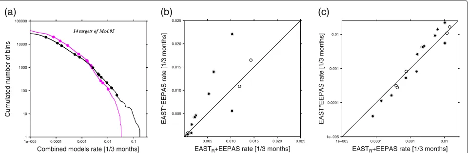
Figure 6a shows the cumulative distribution func-tions of the rates predicted by the EAST∗EEPAS and EASTR+EEPAS models. This plot indicates that the

EAST∗EEPAS model explores a much wider range of values than the EASTR+EEPAS models. In addition, we

observe that more than 50% of target earthquakes occur for only 2% of the highest rates and that, for these events, the rates of the EAST∗EEPAS model are about twice those of the EASTR+EEPAS model. This difference indicates

that the combination based on differential probability gain is currently better than a linear combination at increasing the predicted event rates in the limit of high rate val-ues. Obviously, the opposite is true in the limit of low range value. Nevertheless, in this case, both models fail to predict the target earthquake and a possible gain in trying to combine them is worth discussing. Simultane-ously, these results confirm that the only restriction for performing a combination is the need to use two comple-mentary forecast models, i.e., two models that ensure a nontrivial Molchan diagram with respect to one another (g_inputcurrent>1 in Equation 6).

Figure 6b,c compares the single rate values of the EAST∗EEPAS and EASTR+EEPAS models in space-time

regions where a target earthquake occurred. In the limit of high rates, the rate values of the EAST∗EEPAS model are double those of the EASTR+EEPAS model (Figure 6b).

This demonstrates that a combination of forecast mod-els based on differential probability gains can increase earthquake probabilities in rate-based forecast models.

Conclusions

There are different types of earthquake forecast mod-els, all of which are related to specific sets of observa-tions (e.g., catalogs of seismicity, fault maps, strain rates, and seismic precursors). As illustrated by the outputs of alarm-based and rate-based models, individual forecasts may fall into different classes of statistical models. In this specific context, it is still impossible to combine all types of forecast using ensemble classification methods. Hence, we proposed here a practical method to combine forecasts based on differential probability gains.

(a) (b)

−118˚ −117˚ −116˚ −115˚

32˚ 33˚ 34˚ 35˚

0 100 200

Ea1

EAST

−118˚ −117˚ −116˚ −115˚

32˚ 33˚ 34˚ 35˚

0.000 0.005 0.010 0.015

λ(M≥5)

EAST_R

(c) (d)

−118˚ −117˚ −116˚ −115˚

32˚ 33˚ 34˚ 35˚

0.000 0.005 0.010 0.015

λ(M≥5)

EEPAS

−118˚ −117˚ −116˚ −115˚

32˚ 33˚ 34˚ 35˚

0.000 0.005 0.010 0.015

λ(M≥5)

EEPAS

Figure 4Three-month forecasts of EAST, EASTR, EEPAS, and EAST∗EEPAS models.Three-month forecasts of the EAST(a), EASTR(b), EEPAS(c),

and EAST∗EEPAS(d)models forM≥4.95 earthquakes from April to June 2010 in northern Baja, California along the USA-Mexico border. Blue circles correspond toM≥4.95 earthquakes that occurred in this area during this period. For the EAST model the color map varies from zero to the maximum of the alarm functionEa1(Shebalin et al. 2011). For other models, the same color bar is used to represent the forecast rates ofM≥4.95

earthquakes. Note the higher contrast for the EAST_∗EEPAS forecasts and the increase in event rate in zones where both the EASTRand EEPAS

(a) (b)

0.0 0.2 0.4 0.6 0.8 1.0

miss rate,

ν

0.0 0.2 0.4 0.6 0.8 1.0

τRI

19 targets of M≥5

0.0 0.2 0.4 0.6 0.8 1.0

miss rate,

ν

0.0 0.2 0.4 0.6 0.8 1.0

τRI

14 targets of M≥5

Figure 5Comparison of forecasts of the EAST∗EEPAS and the EASTR+EEPAS models using Molchan diagrams.The tests were done in the entire California CSEP testing region(a)and in a reduced region(b)that does not include off-coast and outside USA areas (Shebalin et al. 2011). Using Molchan diagrams, we compare the forecasts of the EAST∗EEPAS (black lines) and EASTR+EEPAS (magenta lines) models with respect to the

RI reference model. In the linear combination EASTR+EEPAS, the rates issued from both forecast models have the same weight. The dashed

diagonal line corresponds to an unskilled forecast. The shaded area indicates the zone in which the forecast of the tested model outperforms the forecast of the reference model at a level of significanceα=1%. For both combined models, we consider single rate values obtained by summing the expected rates ofM≥4.95 target earthquakes.

related to earthquake phenomena. The quality of the combined model does not have to depend on causal rela-tionships between the different models being combined. Actually, the procedure applies to any forecast models that have additional forecast skill. Nevertheless, since we can-not formulate it in terms of traditional classification prob-lems without a loss of generality, the overall performance of a combined forecast model can only be established on purely empirical grounds.

In contrast to linear methods, our procedure does not average the local expected rates of different models. Instead, it redistributes in space the rates of the current model according to the additional knowledge carried by the input model. Then, as shown by Figure 6, the com-bined model may cover a larger range of rate values, especially in the limit of high rates that are critical for operational forecast. An essential property of this redistri-bution process is to keep constant the total expected rate

(a) (b) (c)

1 10 100 1000 10000 100000

Cumulated number of bins

1e−005 0.0001 0.001 0.01 0.1

Combined models rate [1/3 months]

14 targets of M≥4.95

0.005 0.010 0.015 0.020 0.025

EAST*EEPAS rate [1/3 months]

0.005 0.010 0.015 0.020 0.025

EASTR+EEPAS rate [1/3 months]

1e−005 0.0001 0.001 0.01

EAST*EEPAS rate [1/3 months]

1e−005 0.0001 0.001 0.01

EASTR+EEPAS rate [1/3 months]

Figure 6Expected rate distributions of EAST∗EEPAS and EASTR+EEPAS models.(a)Cumulative distribution functions of the rate values (black for EAST∗EEPAS and magenta for EASTR+EEPAS). Note the logarithmic scale. Dots show the rates in the space-time region where target earthquakes

have occurred during the quasi-prospective test from July 2009 to December 2011. Linear-scale(b)and logarithmic-scale(c)rates of the EAST∗EEPAS model with respect to rates of the EASTR+EEPAS model in space-time regions where target earthquakes have occurred. Open circles correspond to

the entire CSEP testing region; black dots correspond to the reduced region that does not include off-coast and outside USA areas (Shebalin et al. 2011). Thex=yline is shown for direct comparison. The curves in(a)are left-truncated at a rate of 10−5_{per 3 months. The EAST∗EEPAS model has}

of the current rate-based model. This property can be eas-ily demonstrated from simple geometric considerations on the smoothed Molchan trajectories (see Appendix 2 and Figure 2). Nevertheless, if this conservation property is verified for the retrospective period during which the differential probability functions have been determined, it may be only approximate during the quasi-prospective and real-time tests.

The differential probability gain approach can be used to combine successively different forecast models. How-ever, each model brings not only additional information but also some noise. Therefore, changes in the level of noise must be estimated when many models are combined together. In real-time testing, it is practically impossible to quantify the level of noise in individual models because the available case histories are always quite short. Accord-ingly, making theoretical estimates of the overall noise is not yet possible. Instead, we perform numerical experi-ments (see Appendix 3). The test shows that even after 10 iterations with highly noisy simulated models, the result remains quite similar to the original one.

Our combination method is not commutative. To demonstrate this, we analyze the two combined models that can be derived from EASTRand EEPAS models. We

note that the two possible combined models are quite similar. Nevertheless, using Molchan and likelihood tests, we observe that the EASTR∗EEPAS model performs

bet-ter (and is therefore different) than the EEPAS∗EASTR

model. The difference in log likelihood per earthquake is about 0.1.

As shown in Figure 2d,e,f, we obtain nonmonotonic dif-ferential probability functionsg_EASTEEPAS, that is, the highest alarm function values do not always correspond to the highest gEEPAS_EAST values and high peaks may be observed (Figure 2d). Such cases require special attention. For example, it might be that the peaks are caused by after-shocks of a large earthquake. In our particular case, we checked the time and location of the earthquakes cor-responding to the peaks and found only one case of spatial clustering, a swarm of four 4.97 ≤ M ≤ 5.1 events in February 2008 preceded by aM 5.36 event in May 2006 and followed by aM 4.96 event in November 2008. This sequence took place near the epicenter of the future M 7.2 El Mayor-Cucapah earthquake of April 4, 2010. All these M ≈ 5 events are associated with a multiple peak in Figure 2d for AEAST ≈ 2. However, this specific range of alarm function is also associated with 13 other target earthquakes. Hence, we infer that a monotonic character of the differential probability gain functiong is not a necessary condition to combine two models. The gain functions depend on the choice of the learning interval. Some stronger smoothing or approxi-mation might be preferable, particularly for operational forecasts.

The major difference between Molchan and likelihood tests resides in the way the rate variable is weighted. Molchan tests are based on the sum of the expected event rates, whereas likelihood tests are based on the sum of the logarithm of these rates. The comparison of Figure 6b,c illustrates the difference between these two tests:

1. In Molchan diagrams, the relative performance of two models may be measured by the probability gain (see Equation 3, Aki (1981), and Molchan (1990)). For two rate-based models, this probability gain may also be estimated as the slope of the best-fit line in a cross-distribution of the rates (i.e., the diagram in which the rates of one model are plotted with respect to the other where target earthquakes have

occurred). In Figure 6b, this slope is close to 2. In addition, we can graphically verify that events at high rates have more weight than events at small rates in determining this slope.

2. In likelihood tests, the relative performance of two models is expressed as the difference of their log likelihoods per earthquake (Equation 2). If the total expected rates are the same in both models, this is equivalent to the average vertical distance to the diagonal in Figure 6c. In contrast to Aki’s probability gain (Figure 6b), this averaging gives the same weight to all rates. As a consequence, positive distances at high rates and negative distances at low rates cancel each other out.

This comparison highlights the advantage of our method based on Molchan tests. Indeed, good forecasts for low earthquake rates are not as important as for high rates. In fact, earthquakes occurring in space-time regions with low expected rates have to be considered as a ‘failure to forecast’.

Appendix 1

Automatic procedure to estimate differential probability gain functions

Given a finite numberN of target earthquakes and the discretization of space, the Molchan trajectory is a step-like function. To estimate the differential probability gain function, we use a procedure that automatically smooths a Molchan trajectory into Nseg segments. If N ≤ Nseg,

we consider a segment for each step of the Molchan tra-jectory, and the vertical coordinates of the segments are

i/N withi ∈ {0, 1,. . .,N}. IfN > Nseg, we only

con-siderNseg segments, and the vertical coordinates of the

segments are N(Nseg−i)/Nseg/N with i ∈[0,N] and

where x is the largest integer less than or equal to

x. At each step where there is a vertical limit of seg-ments, the horizontal coordinate of the segments is the τ value that corresponds to the median of the distribu-tion of the alarm funcdistribu-tion value for this step. Everywhere in this study, we useNseg = 20 (Figure 2), but we check the stability of the results for 10 < Nseg < 30. From

our experience, we also infer that there is not a strong impact of the smoothing method on the result as soon as

Nseg>10.

Appendix 2

Conservation of the total expected rate in a combining method using differential probability gains

g(A) is the differential probability gain function of the Molchan diagram that evaluates the performance on an input model of alarm functionAwith respect to a rate-based forecast model.λcurrent(x,t)are the expected event

rates of this current version of the rate-based model in the space-time region(x,t). Using our combining method, we calculate the expected event rates of the new rate-based model

λ_new(x,t)=g(A(x,t))λ_current(x,t). (7)

To estimate the differential probability gain function, we smooth the Molchan trajectory using Nseg segments

(see Appendix 1). Let us denote by (τ_i,ν_i) and Ai, i ∈

{0, 1,. . .,Nseg}, the segment extremity coordinates and

the corresponding alarm function values of the input model, respectively. The slope of these segments is the differential probability gain gi, i ∈ {1, 2,. . .,Nseg}. By

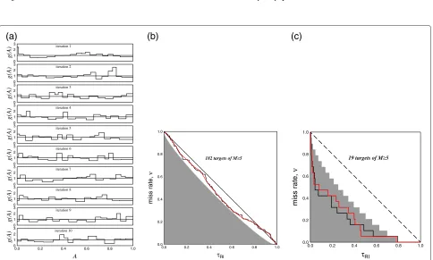
Figure 7Level of noise in combined forecast models using the differential probability gains approach.The EAST∗EEPAS model is successively combined with 10 random rate-based models forM>4.95 target earthquakes (see text).(a)Differential probability gaing(A)

For the current and the new model, we may group the expected event rates according to the ranges of the input model alarm function that correspond to the different seg-ments of the Molchan diagram (Figure 2 and Appendix 1):

λi_current=

where the sum symbols refer to the space-time regions in which the subscript condition is satisfied. We define the total rates of the current and the new models as

current=

For the period in which the differential probability gain function is estimated, we have

λi_current=current(τi−τi−1). (11)

In that case, using successively Equations 7, 11, and 8, we obtain

For a real-time test or a quasi-prospective test, this conservation of the total expected rate is approximate.

Appendix 3

The level of noise in combined forecast models

Taking the EAST∗EEPAS model as the initial forecast model, we study the impact of highly noisy alarm-based models on the next-generation forecasts (Figure 3a). As before, we used the period from January 1984 to June 2009 for learning and the period from July 2009 to December 2011 for testing. For both periods, a single magnitude interval for target events (M≥4.95), and each space-time region, we simulate 10 alarm-based models by drawing random numbers from a uniform distribution between 0 and 1. Then, we iteratively create the next-generation forecasts by incorporating the predictive skills of individual models into the current-generation forecast. As described in Section ‘A differential probability gain approach for combining two earthquake forecast models’ and Appendix 1, theg(A(x,t))values are estimated dur-ing the learndur-ing period (Figure 7a) and then injected into the current-generation forecasts for both periods. For the learning period, Figure 7b shows the Molchan diagram

that compares the forecasts before and after the 7th iter-ation. This iteration exhibits the largest deviation from the diagonal. For the testing period, Figure 7c shows the Molchan diagram that evaluates the predictive skills of the initial and final forecast models with respect to the RI ref-erence model. We find that even after 10 iterations with highly noisy simulated models, the result remains quite similar to the original one. This result is consistent with all the successive Molchan diagrams, which systemati-cally show that two consecutive forecasts have no specific skills with respect to one another. This analysis reveals that, despite an unavoidable increase of noise, there is no systematic erosion of the forecast skills of a model during the combining procedure. Therefore, an obvious recommendation is to avoid combining weak models.

Competing interests

The authors declare that they have no competing interests.

Authors’ contributions

PS conceived, designed, and coordinated the study, conducted the numerical tests, and wrote the manuscript. CN designed the study and wrote the manuscript. JDZ designed the statistical tests and wrote the manuscript. MH designed the statistical tests. All authors read and approved the final manuscript.

Acknowledgements

We are grateful to the editor and the reviewers for their valuable comments. This work was partially supported by the Russian Foundation for Basic Researches, Project No. 14-05-00541. The research was partially performed within the framework of the REAKT Project (Strategies and tools for Real-Time EArthquake RisK ReducTion) founded by the European Community via the Seventh Framework Program for Research (FP7), Contract No. 282862.

Author details

1_{Institute of Earthquake Prediction Theory and Mathematical Geophysics,}

84/32 Profsouznaya, Moscow 117997 Russia.2_{Equipe de Dynamique des} Fluides Géologiques, Institut de Physique du Globe de Paris, Sorbonne Paris Cité, Univ Paris Diderot, UMR 7154 CNRS, 1 rue Jussieu, Paris 75238, France. 3_{Swiss Seismological Service, ETH Zurich, NO H 3, Sonneggstrasse 5, Zürich}

8092, Switzerland.4_{Institutes of Applied and Industrial Mathematics,} Universtität Potsdam, POB 601553, Potsdam 14115, Germany.

Received: 4 December 2013 Accepted: 17 April 2014 Published: 23 May 2014

References

Aki K (1981) A probabilistic synthesis of precursory phenomena. In: Simpson DV, Richards PG (eds) Earthquake prediction. An international Review Manrice Ewing series. American Geophysical Union, Washington, DC, pp 566–574 Aki K (1996) Scale dependence in earthquake phenomena and its relevance to

earthquake prediction. Proc Natl Acad Sci USA 93:3740–3747 Eberhard DA, Zechar JD, Wiemer S (2012) A prospective earthquake forecast

experiment in the western Pacific. Geophys J Int 190(3):1579–1592 Evison FF, Rhoades DA (2004) Demarcation and scaling of long-term

seismogenesis. Pure Appl Geophys 161:21–45. doi:10.1007/s00024-003-2435-8

Gerstenberger MC, Jones LM, Wiemer S (2007) Short–term aftershock probabilities: case studies in California. Seism Res Lett 78:66–77 Hastie T, Tibshirani R, Friedman J (2008) The elements of statistical learning,

2nd edn. Springer (Springer Series in Statistics), New York, USA Helmstetter A, Kagan YY, Jackson DD (2006) Comparison of short-term and

time-independent earthquake forecast models for southern California. Bull Seismol Soc Am 96:90–106

Jordan TH, Jones LM (2010) Operational earthquake forecasting: some thoughts on why and how. Seism Res Lett 81:571–574

Keilis-Borok V, Kossobokov V (1990) Premonitory activation of earthquake flow - algorithm M8. Phys Earth Planet Inter 61:73–83

Keilis-Borok V, Rotwain I (1990) Diagnosis of time of increased probability of strong earthquakes in different regions of the world - algorithm CN. Phys Earth Planet Inter 61:57–72

Kossobokov V (2006) Testing earthquake prediction methods: the west Pacific short-term forecast of earthquakes with magnitudeMw≥5.8.

Tectonophysics 413:25–31

Kossobokov V, Shebalin P (2003) Earthquake prediction. In: Keilis-Borok VI, Soloviev AA (eds) Nonlinear dynamics of the lithosphere and earthquake prediction. Springer, Berlin–Heidelberg, pp 141–205

Marzocchi W, Zechar JD, Jordan TH (2012) Bayesian forecast evaluation and ensemble earthquake forecasting. Bull Seismol Soc Am 102:2574–2584. doi:10.1785/0120110327

Molchan G (1990) Strategies in strong earthquake prediction. Phys Earth Planet Inter 61:84–98

Molchan G (1991) Structure of optimal strategies in earthquake prediction. Tectonophysics 193:267–276

Molchan G (2010) Space-time earthquake prediction: the error diagrams. Pure Appl Geophys 167(8–9):907–917. doi:10.1007/s00024-010-0087-z Molchan G (2012) On the testing of seismicity models. Acta Geophysica

60(3):624–637. doi:10.2478/s11600-011-0042-0

Molchan G, Keilis–Borok V (2008) Earthquake prediction: probabilistic aspect. Geophys J Int 173:1012–1017

Nanjo KZ, Tsuruoka H, Hirata N, Jordan TH (2011) Overview of the first earthquake forecast testing experiment in Japan. Earth Planets Space 63(3):159–169

Narteau C, Shebalin P, Holschneider M (2002) Temporal limits of the power law aftershock decay rate. J Geophys Res 107. doi:10.1029/2002JB001868 Narteau C, Shebalin P, Holschneider M (2005) Onset of power law aftershock

decay rates in Southern California. Geophys Res Lett 32. doi:10.1029/2005GL023951

Narteau C, Shebalin P, Holschneider M (2008) Loading rates in California inferred from aftershocks. Nonlin Proc Geophys 15:245–263

Narteau C, Byrdina S, Shebalin P, Schorlemmer D (2009) Common dependence on stress for the two fundamental laws of statistical seismology. Nature 462:642–645. doi:10.1038/nature08553

Ogata Y (1989) Statistical models for standard seismicity and detection of anomalies by residual analysis. Tectonophysics 169:159–174

Peresan A, Costa G, Panza G (1999) Seismotectonic model and CN earthquake prediction in Italy. Pure Appl Geophys 154:281–306

Rhoades DA (2013) Mixture models for improved earthquake forecasting with short-to-medium time horizons. Bull Seimol Soc Am 103:2203–2215. doi:10.1785/0120120233

Rhoades DA, Evison FF (2004) Long-range earthquake forecasting with every earthquake a precursor according to scale. Pure Appl Geophys 161:47–72. doi:10.1007/s00024-003-2434-9

Rhoades DA, Evison FF (2007) Application of the EEPAS model to forecasting earthquakes of moderate magnitude in southern California. Seismol Res Lett 78:110–115. doi:10.1785/gssrl.78.1.110

Rhoades DA, Gerstenberger MC (2009) Mixture models for improved short-term earthquake forecasting. Bull Seism Soc Am 99:636–646. doi:10.1785/0120080063

Romashkova LL, Kossobokov VG (2004) Intermediate–term earthquake prediction based on spatially stable clusters of alarms. Dokl Earth Sci 398:947–949

Schorlemmer D, Gerstenberger M, Wiemer S, Jackson DD, Rhoades DA (2007) Earthquake likelihood model testing. Seismol Res Lett 78:17–29 Shebalin P, Kellis-Borok V, Gabrielov A, Zaliapin I, Turcotte D (2006) Short-term

earthquake prediction by reverse analysis of lithosphere dynamics. Tectonophysics 413:63–75

Shebalin P, Narteau C, Holschneider M, Schorlemmer D (2011) Short-term earthquake forecasting using early aftershock statistics. Bull Seimol Soc Am 101: 297–312. doi:10.1785/0120100119

Shebalin P, Narteau C, Holschneider M (2012) From alarm-based to rate-based earthquake forecast models. Bull Seimol Soc Am 102.

doi:10.1785/0120110126

Sobolev GA, Chelidze TL, Zavyalov AD, Slavina LB, Nikoladze VE (1991) Maps of expected earthquakes based on a combination of parameters.

Tectonophysics 193:255–265. doi:10.1016/0040-1951(91)90335-P Sobolev GA, Tyupkin YS, Smirnov VB (1996) Method of intermediate term

earthquake prediction. Doklady Akademii Nauk 347:405–407 Taroni M, Zechar J, Marzocchi W (2014) Assessing annual global M6+

seismicity forecasts. Geophys J Int 196(1):422–431

Tsuruoka H, Hirata N, Schorlemmer D, Euchner F, Nanjo KZ, Jordan TH (2012) CSEP testing center and the first results of the earthquake forecast testing experiment in Japan. Earth Planets Space 64(8):661–671

Zechar JD (2010) Evaluating earthquake predictions and earthquake forecasts: a guide for students and new researchers. Community Online Resource for Statistical Seismicity Analysis. pp 1–26. doi:10.5078/corssa-77337879 Zechar JD, Jordan TH (2008) Testing alarm-based earthquake predictions.

Geophys J Int 172:715–724. doi:10.1111/j.1365-246X.2007.03676.x Zechar JD, Jordan TH (2010) The area skill score statistic for evaluating

earthquake predictability experiments. Pure Appl Geophys 167:893–906 Zechar JD, Gerstenberger MC, Rhoades DA (2010a) Likelihood-based tests for

evaluating space--rate–magnitude earthquake forecasts. Bull Seism Soc Am 100(3):1184–1195. doi:10.1785/0120090192

Zechar JD, Schorlemmer D, Liukis M, Yu J, Euchner F, Maechling PJ, Jordan TH (2010b) The collaboratory for the study of earthquake predictability perspective on computational earthquake science. Concurrency Comput–Pract Exp 22:1836–1847

doi:10.1186/1880-5981-66-37

Cite this article as:Shebalinet al.:Combining earthquake forecasts using differential probability gains.Earth, Planets and Space201466:37.

Submit your manuscript to a

journal and benefi t from:

7 Convenient online submission 7 Rigorous peer review

7 Immediate publication on acceptance 7 Open access: articles freely available online 7 High visibility within the fi eld

7 Retaining the copyright to your article