A STUDY OF FOURTEEN YEAR OLD MALAYSIAN STUDENTS' DEVELOPMENT OF GRAPHICAL CONCEPTS WITH TECHNOLOGY
Baiduriah Yaakub
A thesis submitted for the degree of Doctor of Philosophy
Institute of Education University of London
ABSTRACT
This study investigates 14 year-old students' development of graphical concepts using graphing calculators. Two learning models based on two broad interpretations of Vygotsky's "zone of proximal development" were implemented to gauge the role of graphing calculators in technology-based learning. Epistemological case studies were used to ascertain the extent to which the graphing calculator facilitated the learning of key graphical concepts. To this end, students of different levels of mathematical attainment were observed to determine the different kinds of understanding they derived from using the technology.
The 24 students participating in the study were pre and post tested, and formed into two groups. One group was taught according to a structured, teacher-led learning model, and the other group was taught according to an open-ended, activity-led learning model.
What emerges from the study is the complexity of the teaching and learning situation when technology is incorporated. A student's learning of graphical concepts with the graphing calculator was the result of an interplay between his/her knowledge of the functionality of the graphing calculator, existing mathematical knowledge and the nature of teacher intervention.
ACKNOWLEDGMENTS
My thanks go primarily to my supervisor, Dr. Ian Stevenson for having had the patience to guide and assist me through the completion of the thesis. His insights gave me invaluable formative experiences, and his constant encouragement to persevere was a source of inspiration.
My heartfelt thanks also go to my husband, Yusoff, for providing me the moral and financial support, and patiently tolerated my preoccupation with the thesis. To him I dedicate this thesis.
This study would not have been possible without the cooperation of the principal, the teachers and the students at the school where the research was conducted. My deepest thanks to the two teachers who had the willingness, and the courage to try the teaching modules and use the graphing calculator, a tool that they encountered and used for the first time in their teaching career.
I am also particularly grateful to Prof. Celia Hoyles for her critical comments and suggestions.
These acknowledgements would not be complete without thanks to all the staff in the Mathematical Sciences Group whose friendship over the years and helpfulness in so many ways, contributed in creating a supportive working environment.
TABLE OF CONTENTS
Page
Abstract ii
Acknowledgements iii
Table of contents iv
List of appendices viii
List of figures ix
List of tables xi
List of excerpts xii
CHAPTER 1 BACKGROUND
Introduction 1
1.1 Why the graphing calculator? 3
1.2 Graphing in Malaysian schools 5
1.3 Technology and teachers 9
1.4 Aims of this study 10
1.5 Contents of the thesis 10
CHAPTER 2 A REVIEW OF THE LITERATURE
2.1 Graphs and graphing 13
2.2 Misconceptions and difficulties in graphing 16
2.2.1 Linearity 17
2.2.2 Continuity 18
2.2.3 Representations 20
2.2.4 Scaling 22
2.2.5 Variable 23
2.3 The use of a graphing calculator in students' learning 24
2.3.1 Graphical concepts 25
2.3.2 Errors related to graphing calculator use 29
2.3.2.1 Visual illusions 30
2.3.2.2 View-windows 32
2.3.2.3 Tool artefacts 34
2.4 The role of technology in students' learning 39 2.5 The role of the teacher with technology 49
2.6 Conclusion 54
CHAPTER 3 THE THEORETICAL FRAMEWORK
3.1 The Vygotskian perspective on knowledge construction 56 3.2 Different interpretations of the zone of proximal development 63
3.3 The learning models for this study 67
3.4 The study 72
3.5 The research questions 73
CHAPTER 4 METHODOLOGY
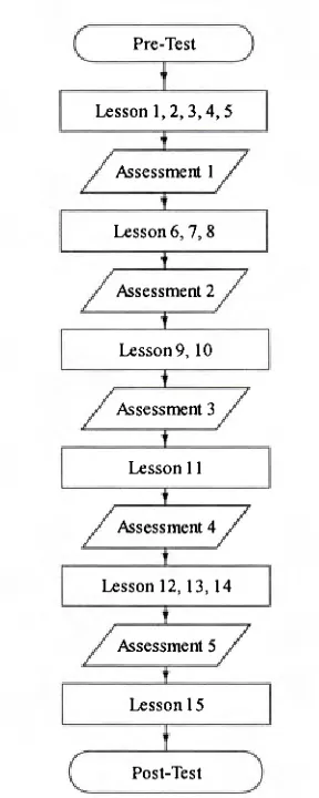
4.1 The design of the study 74
4.2 The design of the lessons 76
4.3 The design of the assessment 82
4.4 Pilot study 84
4.5 Outcomes of the pilot study and implications for the main study 84
4.6 Main study implementation 87
4.6.1 Teacher selection 88
4.6.2 Teacher training 88
4.6.3 Selection of students 89
4.6.4 Videotaping in the classroom 90
4.6.5 Data collection method 90
4.7 The analytic framework 94
4.7.1 Preliminary data analysis 95
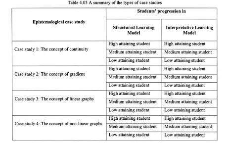
4.7.2 Selection of case study students 96
4.7.3 The case studies 96
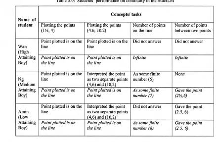
CHAPTER 5 CASE STUDY 1: THE CONCEPT OF CONTINUITY
5.1 Background 101
5.6 Conclusion on the concept of continuity in the Interpretative Learning 139 Model
CHAPTER 6 CASE STUDY 2:THE CONCEPT OF GRADIENT
6.1 Background 140
6.2 Expected learning outcomes with the graphing calculator on gradient 145 6.3 Analysis of case study students in the Structured Learning Model 146 6.4 Conclusion on the concept of gradient in the Structured Learning Model 166 6.5 Analysis of case study students in the Interpretative Learning Model 167 6.6 Conclusion on the concept of gradient in the Interpretative Learning 182
Model
CHAPTER 7 CASE STUDY 3: THE CONCEPT OF LINEAR GRAPHS
7.1 Background 183
7.2 Expected learning outcomes with the graphing calculator on linear graphs 187 7.3 Analysis of case study students in the Structured Learning Model 189 7.4 Conclusion on the concept of linear graphs in the Structured Learning 206
Model
7.5 Analysis of case study students in the Interpretative Learning Model 207 7.6 Conclusion on the concept of linear graphs in the Interpretative Learning 224
Model
CHAPTER 8 CASE STUDY 4: THE CONCEPT OF NON-LINEAR GRAPHS
8.1 Background 226
8.2 Expected learning outcomes with the graphing calculator on 229 non-linear graphs
8.3 Analysis of case study students in the Structured Learning Model 231 8.4 Conclusion on the concept of non-linear graphs in the Structured Learning 242
Model
8.5 Analysis of case study students in the Interpretative Learning Model 243 8.6 Conclusion on the concept of non-linear graphs in the Interpretative 259
CHAPTER 9 FINDINGS AND DISCUSSION
9.1 Mathematical knowledge 262
9.2 Functionality of the calculator 266
9.3 Teacher intervention 268
9.4 The learning models 270
9.5 Models of students' learning 272
CHAPTER 10 CONCLUSION
10.1 The impact of technology on students' learning 276 10.2 The value of using Vygotsky's idea of the zone of proximal development 278 10.3 Implications for the integration of graphing calculators in students' 279
learning
10.4 Limitations of the study and suggestions for future research 281
10.5 Concluding remarks 283
LIST OF APPENDICES
Page Appendix 1 Excerpt of a student's disapproval of the open learning approach 304 Appendix 2 Teaching Module for Structured Learning Model 305
Appendix 3 Teaching Module for Interpretative Learning Model 343 Appendix 4 Students' Worksheet for Structured Learning Model 379 Appendix 5 Students' Worksheet for Interpretative Learning Model 411
Appendix 6 Graphing Calculator Manual 437
Appendix 7 Assessment 1 459
Appendix 8 Assessment 2 460
Appendix 9 Assessment 3 461
Appendix 10 Assessment 4 463
Appendix 11 Assessment 5 464
Appendix 12 Pre-test 466
LIST OF FIGURES Figure 2.01 Figure 2.02 Figure 2.03 Figure 2.04 Figure 2.05 Figure 2.06 Figure 2.07 Figure 2.08 Figure 2.09 Figure 2.10 Figure 2.11 Figure 2.12 Figure 2.13 Figure 2.14 Figure 2.15 Figure 2.16 Figure 2.17 Figure 2.18 Figure 4.01 Figure 4.02 Figure 5.01 Figure 5.02 Figure 5.03 Figure 5.04 Figure 5.05 Figure 5.06 Figure 6.01 Figure 6.02 Figure 6.03 Figure 6.04 Figure 6.05 Page
Graphs of a family of parabolas 15
Item on scaling in the CSMS study 22
Graph of y=-0.5x-2 30
Graph of y=-0.5x+2 30
Graph of y=-2x-3 30
Graph of y=-2x+3 30
Graph of y=-0.5x+2 31
Graph of y=-x-2 in the INIT window 31
Graph of y=-x-2 when "zoomed out" 31
Graph of y=x2-x-1 in the INIT window 31
Graph of y=x2-x-1 when "zoomed out" 31
Graphs of y=5x2-2x+1 and y=5x2-2x-2 32
Graphs of y=2x+3 and y=-0.5x-2.5 in the "standard window" 32
Graph of y=x drawn in different view-windows 32
Graph of y=3x in the standard window 33
Graph of y=3x+400 34
The view-window setting 34
The graph of y=2x3-16x2+12x+6 34
Flowchart of instrument implementation 91
The layout of the classroom and students 92
A view-window with large values 106
A previous view-window 108
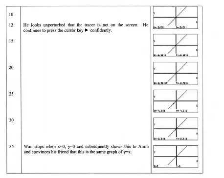
Movement of the tracer from one point to the next point 122
Graph of y=x generated in the G-CON and G-PLT 124
with range values of x from 1 to 6
Effects of the change in pitch value 125
An unusual view-window setting by Grace 125
Graphs of equations with different values of "m" 141
Gradient as the ratio of (y2-yI) to (x2-xi) 141
Graphs of (+1, y=x and y=x-1 in two different view-windows 147
Wan's sketch of graphs with different gradients 149
Figure 6.06 Ng's sketch 155
Figure 6.07 Ng's hand draw graphs of y=mx 158
Figure 6.08 Graphs of y=Mx generated in the DYNA Mode 164
for range of values of "M" between —3 and 3
Figure 6.09 Emy's imperfect STARBURST picture in the STD window 180
Figure 7.01 Replication of the graphic display 197
Figure 7.02 Amin's work on determining the gradient 204
Figure 7.03 "Graph Func" syntax on both screens 215
Figure 8.01 The parabola generated in the G-PLT and G-CON command 230
LIST OF TABLES
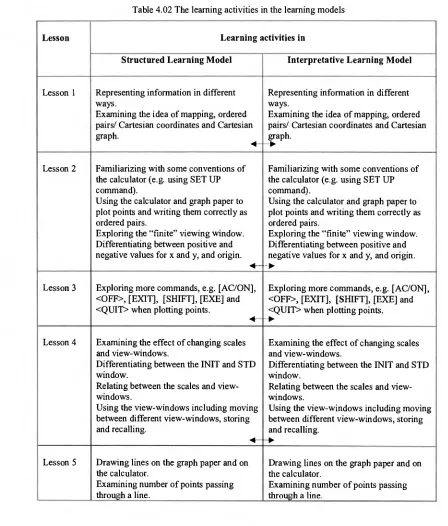
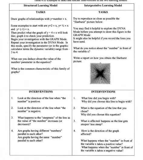
Page Table 4.01 Differences between the Structured and Interpretative 75
Learning Model
Table 4.02 The learning activities in the learning models 77 Table 4.03 Example of tasks and teacher interventions in the two 81
learning models
LIST OF EXCERPTS
Page Excerpt 5.01 Wan's understanding of the trace facility and number sense 105 Excerpt 5.02 Wan's understanding of the view-window in relation to 107
the movement of the pointer
Excerpt 5.03 Ng's understanding of the view-window and tracer 111 Excerpt 5.04 Ng's understanding of the view-window in relation to 114
the appearance of the graph
Excerpt 5.05 Ng's difficulty with the tracer 115 Excerpt 5.06 Amin's difficulty with choosing a view-window 119 Excerpt 5.07 Teacher intervention with Grace 126 Excerpt 5.08 Presha's difficulty with the calculator operations 128
Excerpt 5.09 Presha's difficulty with the TABLE Mode 130 Excerpt 5.10 Emy's difficulty with the mathematical terms 133 Excerpt 5.11 Emy's difficulty with the functionality of the TABLE Mode 135 Excerpt 6.01 Wan's understanding of the functionality of the DYNA Mode 148
Excerpt 6.02 The influence of Wan's mathematical language 150 Excerpt 6.03 The influence of Wan's algebraic competency 152 Excerpt 6.04 The graphing calculator as a display tool 154 Excerpt 6.05 Ng's difficulty with the DYNA Mode 156 Excerpt 6.06 Teacher's ineffective intervention 161 Excerpt 6.07 Knowledge compartmentalisation arising from difficulty 165
in making sense of graphic display
Excerpt 6.08 Grace's understanding of the DYNA Mode 168 Excerpt 6.09 The influence of Grace's mathematical knowledge 169
Excerpt 6.10 The graphing calculator as a display tool 172
Excerpt 7.01 Using the graphing calculator to support conjectures 189 Excerpt 7.02 Wan's ability to follow the curriculum script 190 Excerpt 7.03 Ng's inability to follow the curriculum script 194 Excerpt 7.04 Amin's lack of mathematical knowledge 200 Excerpt 7.05 Amin's lack of consciousness on what is keyed in 204 Excerpt 7.06 Grace's knowledge in decimals and fractions 208 Excerpt 7.07 Teacher's corrective feedback on syntactic error 210 Excerpt 7.08 Presha's inability to make sense of the graphic display 212 Excerpt 7.09 Intervention that did not resolve Presha's difficulty and 214
syntactic error
Excerpt 7.10 Intervention that focuses on obtaining the correct answer 217 Excerpt 7.11 Emy's difficulty in hand graphing 220 Excerpt 7.12 Teacher's scaffolding in Emy's exploration of graphs of 222
y=mx+c
Excerpt 8.01 Transformation in Wan's activity 232 Excerpt 8.02 Inappropriate use of calculator facility 235 Excerpt 8.03 Using the graphing calculator as a display tool 238
Excerpt 8.04 Grace's specific questions 243
Excerpt 8.05 Interpretation of the graphic display 245 Excerpt 8.06 The quality of teacher's knowledge 246 Excerpt 8.07 Knowledge source from classroom teaching 247 Excerpt 8.08 Intervention on semantic error and Presha's difficulty 250
with the task
Excerpt 8.09 The impact of the quality of the teacher's knowledge 251 Excerpt 8.10 The influence of lack of mathematical knowledge 254
CHAPTER 1
BACKGROUND
Introduction
Education occurs within a sociocultural context of which technology is an integral part, that continues to evolve and therefore cannot be ignored. In mathematics education, it has been documented that technology can perform a wide range of mathematical work including algebraic manipulation, solving equations, finding integrals and derivatives, and plotting graphs, thereby having an impact on the mathematics learnt in school. Such technology stimulates an ongoing debate about the appropriate content and organization of the mathematics curriculum when technology is used. More importantly the capability to provide different ways of calculating, and therefore new opportunities for analyzing and solving problems, makes technology a vehicle to transform the teaching and learning process itself. However, technology in and of itself will not change the way teachers teach and the way students learn, what matters is how technology is used (Sandholtz et al., 1997). If it is used in a "meaningful" way, it can transform learning (Sandholtz et al., 1997; Doerr and Zangor, 2000), offering different ways and opening new doors in the teaching and learning of mathematics. Meaningful here means involving the learner, encouraging autonomy, and engagement in questioning, and reflection (Burton and Jaworski, 1995). The challenge therefore is to examine how and to what extent a particular technology can offer support in students' learning. Correspondingly, how can technology be integrated in the classroom: what is its role and what is the role of the teacher in relation to it?
till 1995 (Pusat Perkembangan Kurrikulum, 1995). The SMART School' curriculum (Ministry of Education Malaysia, 1997), to be implemented in stages from 1999 further stresses "moving away from memory-based learning" (p. 9) and catering for individual abilities in the form of technology-supported learning.
The use of scientific and graphing calculators is non-existent in Malaysian secondary schools. Four function calculators are used in secondary schools as a tool to aid in computations, but in general, the use of calculators has no place in mathematics learning. The almost negligible impact of calculators in mathematics classrooms in Malaysia may be attributed to two major reasons. First, simple four function calculators are allowed in the public examination only at the Sijil Pelajaran Malaysia level, taken at the end of the fifth year in secondary school by seventeen year-olds. In Mathematics, calculator use is restricted to one of the two papers taken in which all questions are of "problem-solving" type. Second, the Mathematics Syllabus for secondary school implemented in 1989 preceded the policy on allowing the use of simple calculators in the Sijil Pelajaran Malaysia examination in 1995. The syllabus had not explicitly stated nor suggested that
calculators can be used as a teaching tool in the teaching and learning of mathematics (Pusat Perkembangan Kurikulum, 1989a, b, c; 1990a, b). Since the purpose of calculators in the examination is to aid in carrying out the four basic operations and their use restricted to straightforward computations, calculators in classrooms are also used only to expedite or to check computations. There is very little acknowledgment of their potential in supporting knowledge construction and understanding. It is thus challenging in the Malaysian context to carry out research using graphing calculators, an evolving personal technology considered by many to have the potential to revolutionize mathematics education (Dick, 1992; Ruthven, 1992, 1996; Oldknow, 1995; Waits and Demana, 1996; Slavit, 1996; Barling, 1997; Waits, 2000).
Although graphing calculators are suggested in the SMART School curriculum, the lack of empirical evidence of their potential, and lack of support and know-how for integration in the mathematics classroom renders them almost useless to the teachers. Having the technology resources in the school does not necessarily imply that teachers will use them in their teaching (Norton et al., 2001). Indeed, teachers require the opportunity to look at new developments and examples of technology as used in educational practice so that they become aware of the opportunities they offer (Reys and Smith, 1994; Dawes, 2001).
1.1 Why the graphing calculator?
It is argued that for technology to have any impact on the curriculum and the way teachers teach, the contact time between the students and the technology must be considerable (Doerr and Zangor, 2000; Selinger, 2001). This is a vital question of accessibility when integrating technology in the curriculum — how well is it distributed among students and is it readily available or restricted to a laboratory setting? Studies have indicated that an important factor in the general acceptance of technology by teachers is the availability and portability of the technology (Blease and Cohen, 1990; Martin, 1991; Schmidt and Callahan, 1992). The Chicago Mathematics Project (Usiskin, 1993) reported that calculators were easier to integrate into secondary school mathematics compared to computers, citing problems of access to computers at the required times. The same situation can be argued for many schools nowadays in Malaysia, in particular schools in rural areas that lack the necessary infrastructure for computers. The use of graphing calculators seems more viable. They are not only portable, they are relatively cheaper and robust (Shumway, 1990; Oldknow, 1995; Ruthven, 1994a; Goldstein, 1994; Waits and Demana, 1996; Graham and Thomas, 1997; Berger, 1998) and flexible in terms of time and use (Usiskin, 1993, Hennessy et al., 2001). While this renders them more accessible and thus attractive for frequent use, as Ruthven (1995, 1996) recommends, like any other technological tool their value lies in how they can be used to facilitate teaching and learning. This is precisely what this study sets out to do: to characterize the transformation in students' understanding of mathematical concepts when using the graphing calculator in their learning.
Dick and Shaughnessy, 1988; Graham and Thomas; 1997; Hennessy et al., 2001). This has great implications for dealing with the student attitudes that are increasingly seen as crucial factors affecting their school performance (Schoenfeld, 1989; Galloway et al., 1996).
1.2 Graphing in Malaysian schools
Leinhardt et al. (1990) note that the way equations (functions) and graphs are introduced to students in schools varies from country to country with no proven optimal approach. Since the present study has been developed in the Malaysian school context, the way graphing is approached there will be briefly described. It is useful to point out that, in general, the mathematics curriculum is structured according to content-by-process matrices, in which a list of mathematical topics is outlined as content corresponding to some variant of the Bloom taxonomy2 as process (Pusat Perkembangan Kurikulum, 1989a, b, c; 1990, a, b).
Graphing starts in the elementary school and is approached as the display of information in the form of bar graphs, pictographs, circle graphs and line graphs. It is only in Secondary 2, students are taught to plot points on the Cartesian axes (14 year olds), moving on to linear equations in Secondary 3. The concept of the straight line and its equation y=mx + c is covered in Secondary 4. Graphing of other equations restricted to certain polynomials, namely quadratic, cubic and reciprocal is covered in Secondary 5. This is extended to solving equation(s) by graphical methods and determining the region of an inequality in two variables. It is also expected that over time, students should become able to relate certain types of equations with certain standard shapes of graphs, and vice versa, for example, straight line, parabola, cubic and exponential.
Students also do graphing work in their science and other classes. In science, the graphing work usually starts with the data obtained from observation, which is set up as axes construction, points plotted and finally a graph. Graphs are sometimes plotted to identify the existence of a pattern and hence deduce a relationship, or to predict on the outcome of a variable under consideration. Emphasis is on the qualitative interpretation
2
of graphs, that is, looking at the graph to a relationship between the two variables. This is different from what is learned in the mathematics classroom where graphing work usually starts from a given algebraic function to generate ordered pairs for a graph. In geography, students are acquainted with pie charts, bar graphs, line graphs or other kinds of frequency graphs. These graphs often only consider one continuous variable (frequency), with the other axis used to show entirely independent items. Students also encounter the ideas of dependence and variables in separate mathematical topics like ratio and proportions. However, such diverse ways of thinking about graphs do not necessarily facilitate students' understanding (see e.g., Leinhardt et at., 1990; Demana et al., 1993).
My concern with the Malaysian curriculum is that the way it is structured is based on the notion that mathematical learning is hierarchical from "low level" skills to "high level" skills, illustrated for example in its approach to graphing from "simple" linear equations to the supposed more "difficult" higher order polynomials. Graphing is also treated in a fragmented way, presented in bits and pieces, for example, in Secondary 2 students begin to plot points and stop at the determination of the length and the mid-point of a line between two points. It is not until the following year that they begin to draw graphs of some linear equations, and only after that are they formally introduced to the general form of equation for the straight line (y=mx+c). Graphs of higher order polynomials are not introduced until another year later. As graphing technology is not used in the learning of graphs, it is common that many graphs of equations of higher order are not explored as this is tedious and time consuming to do. Likewise, the investigation of the properties of graphs of different families is also restricted.
Many have argued that the limited opportunity for students to explore graphs of different polynomials, and to manipulate and compare graphs of the same family, is the root cause of students not recognising the form of an equation and its associated graph (Swan, 1982; Demana et al., 1993; Philipp et al., 1993; Kieran, 1993), and students having a local rather the global view of the graph (Demana et al., 1993; Kieran, 1993). The limited opportunity to explore and manipulate graphs deprives students from making connections across the three "multiple linked representations" in graphing (algebraic, tabular or numerical, and graphical) (Goldenberg, 1988; Demana et al., 1993; Moschkovich et al., 1993; Kieran, 1993; Wilson and Krapfl, 1994). Students are also obscured from seeing the equation and the graph as objects or entities that can be manipulated as a whole to form new objects as described by Sfard (1991). Sfard's object or structural conceptualisation3 is useful because it emphasises the importance of detaching the new entity from the process that produced it. In this way, the process of generating a graph has been criticised as one of the factors that obscures students' understanding of graphing. The time spent graphing by manually plotting individual
points obscures the connection between the equation and the graph as "object" (Dick, 1992). As Swan (1982) suggests, these disconnections result in students losing sight of the meaning of graphing tasks.
The advent of graphing technology has been seen as providing a new opportunity for students to explore graphs and to facilitate the forming of connections across representations. Yerushalmy and Schwartz (1993) claim that the use of graphing technology "frees users from the physical action of plotting. This, in turn, may permit them to shift the focus of their attention away from the detail of the process of making the graph and allow them to benefit from the contemplation and manipulation of the graph itself' (p. 46). They also argue that graphing technology which allows the learner to manipulate the graphical representation itself (e.g., to "stretch" or "squeeze") and to view the impacts of this on the numerical and symbolic representations, or those that allow the user to manipulate the numerical representations and view the result in the graph and the symbolic expression, make it more possible for the learner to view the function and any of its representations as a single entity. It must be pointed out that the current graphing calculator technology is restricted in terms of this kind of interactivity. It cannot provide feedback to the user and the graphs it produces cannot be physically and directly manipulated, for example, rotated, pushed or pulled. Therefore "direct graphing action" described by Smith and Confrey (1992) with the computer software Function Probe, in which the user can "create" an action as a visual experience, taking transformations "back" to their geometric origin, or those mentioned above are not possible with the graphing calculator. However, the graphing calculator in the dynamic mode does enable the user to see what happens to a graph when parameters are changed. This dynamic capability has been argued to provide an environment that enables the user to see graphs as objects that can be transformed, thus drawing students' attention to the graph globally (Goldenberg, 1988).
and can inhibit certain kinds of understanding. It can engender certain misconceptions and cause interruption in learning. Some researchers have warned of the potential pitfalls of the graphing tools (e.g., Dion, 1990; Kaput, 1992; Demana et al., 1993), and others have provided evidence of a number of misconceptions that students develop when using these graphing tools (Goldenberg, 1988; Dugdale, 1993; Moschkovich et al., 1993; Ward, 2000). Against the backdrop of the limitations and potentiality of the graphing calculator, it is interesting to see how the graphing calculator facilitates students to understand the relationship between the equation and the graph it represents. To what extent does using the graphing calculator afford the viewing of graphs globally? Does this global view facilitate students' understanding of graph transformations when the parameters in an equation are varied?
1.3 Technology and teachers
There are broadly two main choices for integrating technology into learning. One way is to use it as add-on to facilitate the teaching and learning of some concepts predefined by the curriculum. Alternatively, one can take advantage of the tool's ability to effect deeper changes in the way students learn and the concepts that they learn. Whichever way technology is adopted, the introduction of technology arguably will affect the role of the teacher. For example, the concern towards getting students to be more autonomous and to self-regulate their learning has resulted in some studies that use technology to provide learning environments for student-directed exploration. Hoyles and Sutherland (1989) found that there is a critical balance between teacher-initiated activities and student-directed exploration in student's learning. Student's progress or lack of progress in some areas was found to be closely associated to the presence or absence of appropriate teacher intervention. Noss and Hoyles' (1996) idea of the phenomenon of "didactical paradox" in which "didactical situations 'force' teachers to tell the students what to do; yet the same process empties the learning situation of any cognitive content..." (p. 70), cautions us to be mindful of the role of intervention in student's learning.
interventions promote and complement graphing calculator use that enhance students' learning?
1.4 Aims of this study
Against the backdrop of the Malaysian secondary school year (14 year-old students), this study therefore sets out to investigate:
• the graphical concepts that students can come to understand with the graphing calculator;
• the role of the graphing calculator in facilitating understanding of graphical concepts;
• the extent to which different learning environments in which the graphing calculator is being used structure student's learning;
• the student's approach to using the graphing calculator in his/her learning (including the strategies used when encountered with difficulties and errors operating the calculator); and
• the nature and consequences of teacher intervention in the learning process.
What is needed is a model of teaching and learning with technology which will enable exploration of these issues. A major aspect of this study will be to develop an appropriate framework.
1.5 Contents of the thesis
Chapter 2 presents a review of literature for this study. It starts with defining the meaning of graphs and what constitute as "graphing". Difficulties and misconceptions that are encountered in the learning of graphing concepts are discussed. Included are issues related to graphing calculator use. The role of technology in student's learning and the role of the teacher when technology is used are reflected upon.
explained. The rationale for using the Vygotskian view on knowledge construction is discussed and, drawing from two broad interpretations of Vygotsky's idea of the ZPD, two learning models are proposed for use in this study. The two learning models are defined. This chapter concludes by defining the scope of the study and the research questions.
Chapter 4 describes the methodology employed in the study. It begins by presenting the design of the study, and follows with the design of the lessons used in the study. This chapter also illuminates the test instruments used, their design and the purpose of each instrument. Problems encountered in the pilot study are discussed in relation to their implications for the main study. The student sample of the study and its method of selection are also described. The criteria for choosing the teachers to participate is also discussed. A description of how the learning models were implemented in the classroom and how the classroom was organized to enable the recording of data for the study, is included. How the analytic framework, which follows an iterative design was developed is discussed. This chapter concludes with a description of the use of epistemological case studies to analyze the ways in which the graphing calculator facilitated the learning of particular graphical concepts.
Chapters 5, 6, 7 and 8 are each analysis of case study of the graphical concepts of continuity, gradient, linear graphs and nonlinear graphs respectively. Each case study analyzes how students of different mathematical attainment in each of the two learning models learned with a graphing calculator.
Chapter 9 follows with a discussion of findings of the study framed within its theoretical considerations. It also attempts to model the different kinds of understanding that students derived from using the technology, and concludes with an overview of the complexity of teaching and learning situations when technology is integrated into students' learning.
CHAPTER 2
A REVIEW OF THE LITERATURE
This review is organised into six sections. The first section discusses the meaning of graphs and graphing, and issues surrounding its learning. Section 2.2 discusses the difficulties as well as misconceptions that are encountered in the learning of equations and their graphs. Section 2.3 considers factors related to the use of graphing calculators, including student learning of graphical concepts, errors in graphing calculator use, and issues of instructional approaches when integrating graphing calculators into learning. This is followed with a discussion on the role of technology in student's learning with a focus on the role of graphing calculator in section 2.4. Section 2.5 discusses the role of teachers with technology to highlight issues surrounding integrating technology in classrooms. The conclusion of the review is presented in section 2.6
2.1 Graphs and graphing
The learning of graphs is problematic and this is well-documented (e.g., Kerslake, 1981; Bell et al., 1987; Goldenberg, 1988; Friedler and McFarlene, 1997; Swatton and Taylor, 1994; Romberg et al., 1993; Knuth, 2000). Dictionary definitions describe a graph as a diagram or picture that shows the relationship between two or more quantities (Flyfield and Blane, 1994), or between two variables (Nelson, 1998), where the relationship is shown by means of points plotted on a coordinate system (Tapson, 1996) whose coordinates satisfy the relation (Collins Dictionary, 1995). Fry (1984) proposed a generic definition: "A graph is information transmitted by position of point, line or area on a two-dimensional surface" (p. 5), including all spatial designs and excluding displays that incorporate the use of symbols such as words and numbers (e.g., tables).
vocabulary of graphical language. Therefore, graphs can also be viewed as a form of symbolism with its own syntax and mode of representation (Barclay, 1987; Mokros and Tinker, 1986). Ponte (1987) points out the importance of the global-visual properties of graphs that allow an expert to see at a glance the general features of a relationship. Drawing on these two aspects, Stevenson (1990) proposes that graphs are, therefore, systems of symbolic representation with global-visual properties. Thinking of graphs in this way helps to establish a focus on these two aspects of graphs, which pose particular difficulty in students' learning of graphical concepts.
While there are many types of graphs such as bar graphs and pictographs, the study reported in this thesis is concerned (mainly) with Cartesian graphs. These graphs are drawn using a Cartesian coordinate system, in which the position of a point is determined by its relation to reference lines called axes that are normally at right angles to each other. Descartes (1596-1650) proposed the idea that the relationship between two variables could be visualised by representing the corresponding set of values on a coordinate system. The graph (a line or a curve) can be expressed algebraically as an equation of two variables. Therefore, pairs of values of the algebraic variables in any equation can be represented or interpreted as points on a line or a curve. The curve that is drawn in a coordinate system for a particular equation is the graph of the equation. Conversely, by picturing or representing the related sets of values of two variables as ordered pairs of numbers on the x-y plane, the relationship between the two variables can be visualised through the graph.
have a good idea of the appearance of the graph of a function. This requires the ability to focus on the major features, such as the domain and range, roughly where the roots may occur, whether points of zero gradient are local maxima, minima or neither, and the occurrence of asymptotes and discontinuities. A graph, which is plotted from a table of values for only a comparatively short interval on the x-axis may miss some of these important features of the function. Taking into account a large interval is tedious and may still not produce the complete graph of the function. A complete graph of a function is a graph that shows all its important behaviour such as its y-intercept, zeros, relative extrema, and end behaviour (Demana et al., 1993). A sketch graph can, by distorting the scales on the axes, concentrate on these major features. However, to acquire the skill of graph sketching requires the ability to have some kind of expectation of what the graph of the given function or equation will look like (Stevenson, 1990).
It is obvious that students have to learn to recognise the different forms of the equations and their corresponding general shapes of graphs. Certain standard forms of equations give rise to certain standard shapes of graphs, for example straight line, parabola, sine curve, and exponential. To understand the connections between equations and their graphs, it is helpful to draw some members of a "family" of equations. The example below (Figure 2.01) shows some members of a family of parabolas, identical except for horizontal translation.
y
Figure 2.01 Graphs of a family of parabolas
graphing technology is thought to be able to offer students an alternative way of generating graphs and investigating the different shapes of graph associated with forms of equation (Goldenberg, 1988; Shumway, 1990; Yonder Embse, 1992; Kieran 1993, Fox, 1998; Hennessy et al., 2001).
This study is concerned only with graphs drawn in the Cartesian coordinate system. This means graphs of polynomial equations (including linear, quadratic, cubic quartic and quintic equations); trigonometric equations; logarithmic and exponential equations are investigated. These graphs may be graphs of functions or may not be graphs of functions, as in the case of circles, ellipses, etc.
2.2 Misconceptions and difficulties in graphing
It has been noted that there are salient features of the graphing domain such as scale, gradient and symbolism that cause misconceptions and confusions among students. Goldenberg's (1988) seminal work on graphical representations shows that graphs have ambiguities of their own, and that students often make significant misinterpretations of what they see in these representations. Thus, in order to understand the ways in which the graphing calculator supports (or does not support) students' development of graphing, it is imperative to look at the kinds of difficulties that students encounter in graphing without technology and the probable reasons for these difficulties, and to see whether these misconceptions and difficulties persist in a technology-supported learning environment. It will be useful here to distinguish between difficulties and misconceptions as there may be a particular misconception as the source for an observed difficulty. The distinction provided by Leinhardt et al. (1990) is used here: misconceptions are erroneous features of student knowledge that are repeatable and evident. Difficulties are learning problems related to particular features of graphs and the graphing activities. However, since difficulties and misconceptions are intertwined, they are discussed here together.
concepts are not mutually exclusive, and do overlap with each other. The role of graphing technology in confronting these misconceptions and difficulties is also considered.
2.2.1 Linearity
Several studies have pointed out students' predisposition toward linearity in both abstract and contextualised situations, where students tend to produce linear graphs when asked to connect two given points (Dreyfus and Eisenberg, 1983; Markovits et al. 1983). Markovits et al. (1983) explained this as stemming from students' over-generalisation of the special property of linear functions, that a line is uniquely determined by two points. The propensity toward linearity is also evidenced on translation tasks. For example, Zaslaysky (1987, cited in Leinhardt et al., 1990) found that students used only two points out of the three labelled points of a parabola to determine its equation. They erroneously used them to calculate the slope of the straight line through these two points and substituted the calculated value into the leading coefficient of the equation for the parabola.
anecdotal evidence of a pair of students who seemed to be progressing well in determining equations of polynomial graphs in a technology-supported learning environment. They recognised the effects of the various terms in a graph and had worked out on their own the idea that the constant term is the y-intercept and successfully matched a variety of graphs of polynomials of degree 6 or less. Nevertheless, they erroneously thought that the constant term was the vertex of the given parabola.
The ease of graphing provided by graphing technology means that graphing does not necessarily have to be confined to linear equations at the beginning of the learning sequence. However, it is interesting what forms of difficulties and misconceptions still persist when a graphing calculator is used (see section 2.3).
2.2.2 Continuity
Students' early experiences with graphing may have contributed towards their tendency to focus on individual points. In particular, it is claimed that the early experience with graphing, which is heavily dominated by point-plotting activities, leaves many students with the misconception that curves are not continuous (Herscovics, 1989; Leinhardt et al., 1990; Demana et al., 1993). Arguably the early encounter with graphing in the form of graphing discrete quantities may have resulted in some students developing a fixation4 that graphs are made up of identifiable discrete points. Demana et al. (1993) observed that the continuity of the line is never explicitly taught even at Grade 8 level. There is no mention that a line is continuous or infinite or that a point is on the line if and only if its coordinates satisfy the equation.
The propensity towards individual points hinders students from developing a coherent understanding of the line concept. As argued by Leinhardt et al. (1990) although lines are accepted as a legitimate part of graphs, they only serve to connect the points rather than having a meaning in their own right, and this is seen to be in conflict with viewing a graph as an object or as a conceptual entity. It also obstructs from viewing the graphs globally, which is essential in understanding the gradient concept (Kerslake, 1981) and the idea of transformation (Goldenberg, 1988). For example, Kerslake showed that only a third of the fourteen-year old students sampled realised that the gradient of the straight line was the same at all points on the line.
It is yet to be explored whether the presence of graphing technology can facilitate students to understand the idea of continuity at middle school level. The graphing calculator enables the user, within the limits of its readability, to trace the points (by using the TRACE cursor) on the line with the coordinate values displayed on the screen. The question remains whether students recognise that it is impossible to trace every point that lies on the line and between any two points on the line.
2.2.3 Representations
Making connections between the three different representations: algebraic, tabular and graphic is seen as crucial in understanding about graphing. Moschkovich et al. (1993) however, propose that this should include thinking simultaneously from an object and process perspectives. "From the process perspective, a function is perceived of as linking x and y values: For each value of x, the function has a corresponding y value" (p. 71). Having the process conception of a function is understood as being able to, for example, substitute a value for x into an equation and calculate the resulting value for y or being able to find a solution to an equation by choosing any point on its graph. On the contrary, "from the object perspective, a function or relation and any of its representations are thought as entities - for example, algebraically as members of parameterized classes, or in the plane as graphs that, in colloquial language, are thought as being "picked up whole" and rotated or translated" (p. 71). For example, having an object conception of a function means that one could recognise that equations of lines with the form y=3x+b are parallel. According to Moschkovich et al., understanding connections between these perspectives enables one to view a graph or an equation both as a whole and as being made up of many individual points or ordered pairs.
come to grips with the "Cartesian Connection". That is, the ability to interpret the meaning contained in the statement: "A point is on the graph of the line L if and only if its coordinates satisfy the equation of L". For example, students can treat the algebraic and graphical representations as two different domains. Although they may refer to "m" in the equation y=mx+c as the slope, they may not ascribe it to the "slope-related graphical properties" to equations with varying values of "m" (see section 6.1 for details). Similarly, the student may refer to the "c" value of the equation as the y-intercept, but may not know that the point (0,c) lies on the graph of the equation despite using the term y-intercept to refer to a property of the graph. Students may also not realise that one can change one of the parameter while leaving the other constant and thus generate a family of lines with specific properties. This resonates with the problem of "fixation" reported by Bell et al. (1987) of how some pupils concentrate on only one aspect of some given data and do not coordinate this with other aspects, resulting in difficulties such as interpreting gradients. Also possible is a fixation on changes in the y variable when the relationship between x and y should have been considered.
Students also have difficulties in making connections between tables and graphs. Olsen (2000) points out that the form and constitution of a table of ordered pairs and its graph are quite different. In the table, each ordered pair consists of two numbers whereas on the graph, each point is a single geometric object. Students often do not make the connection that each point stands for an ordered pair (Goldenberg, 1988). The tabular and graphical representations in themselves pose an ambiguous situation. The table is a sampling of some of the ordered pairs whereas the graph contains all the ordered pairs (Olsen, 2000). The fact that the table has a finite number of ordered pairs and the graph has both the calculated ordered pairs and a line or curve drawn through the points results in students not seeing the meaning of the line or curve through the points.
corresponding ordered pairs on the "plotted points" graph and thus better understand the relationship (Vonder Embse and Engebresten, 1996). In addition, the graphing calculator also provides the user the facility to toggle the "points" graph with the corresponding continuous graph. This feature seems to have the potential to directly show students the equation-table-graph translation.
2.2.4 Scaling
Scaling requires attention to the axes: their scales and units. It involves choosing the length of the unit interval and whether both axes have the same scale. Some student misconceptions and difficulties have been traced to a confusion with scaling. Understanding of graphs requires students to know which features of the graph do not change when the scale changes and which features do change when the scale is altered. Some students thought it is legitimate to construct different scales for the positive and negative parts of an axis (Kerslake, 1981), while some students believe that the scales on the x and y axes have to be equal (Cavanagh and Mitchlemore, 2000; Goldenberg, 1988). In the interpretation of a graph, the inclination and shape largely depends on the choice of scales in the coordinate system. Students have to be able to differentiate which features are tied to the graph itself (for example, the x-intercept, the y-intercept) and which features are tied to the coordinate system on which it is created (the slope and consequent appearance of the graph). The Concepts in Secondary Mathematics and Science (CSMS) study (Kerslake, 1981) found that students have difficulty in recognising the effect of changing scales on the appearance of a graph. When asked which two straight line graphs in figure 2.02 show the same information, only 46%, 63% and 68% respectively for 13, 14 and 15 year olds were successful.
y axis x-0 5_
(a) 4— 3— 2—
011.111
1 2 3 4 5 x axis
y-
yaxis 010-
0-
6- (b) 4-
2—
41
4 11 5 2 3
x axis
y axis
x-010— (c) 8— 6— 4— 2
0 4 41
4 1 5 1
1 2 3 x axis
Changes of scale are one of the main sources for graphical visual illusion (Goldenberg, 1988). Such visual illusion becomes particularly critical when using graphing technology, since the technology easily produces many different graphical representations of a single function or equation (Goldenberg, 1988). For example, Vonder Embse and Engebresten (1996) describe a situation where a pair of perpendicular linear graphs does not appear at right—angles on the calculator screen because of unequal scales. Goldenberg (1988) discusses how changing one of the axes can suggest to students that a graph has shifted up or down, or to the left or right. This is discussed in detail in section 2.3.1.
However, it is the capability of the graphing calculator to generate the same graphs easily in different "view-windows" that makes the effects of scaling salient. Hector (1992) suggests that students continually work with "scale" when they look for complete graphs. They also see that parabolas can be made "fat" or "skinny" by varying the x scale. In conventional hand graphing, there is usually just one graph of a particular equation and drawn by choosing the appropriate scale within the boundaries of the graph paper. With graphing technology, students can easily choose to generate the same graph drawn on different scales. This allows easy exploration of the invariants of the graph such as the slope, the intercept, the maxima and the minima but also potential ambiguities.
2.2.5 Variable
variable and the parameter(s) in an equation. This is significant in the case of polynomials as the parameters also affect the shape of the graph. Goldenberg (1988) warns that students who explore the effects on the graph of, say, y=ax2+bx+c as they vary the values of a, b and c may actually misconceive that these values are the variables.
Goldenberg cautions that many graphing technologies do not differentiate between variables and parameters, which may further obscure rather than clarify this difficult concept. Many graphing technologies, including the graphing calculator, generate graphs automatically from left to right, traversing over a set of values of x without any student intervention, and only leave the student to manipulate the equation's parameters. The variable x appears not to be understood as the independent variable by the students, but rather the parameters as they explore the effects of varying the values of a, b, and c on the graphical output. To what extent the variable concept influence students' understanding of graphing concepts in a technology-supported learning environment remains unclear.
Summing up, some of students' difficulties and misconceptions arise within the knowledge of graphing domain itself. However, what emerges from this review is that the way students are taught, with emphasis on point plotting and rarely on the global view of a graph, can exacerbate the problems. According to Dick (1992), using graphing calculators will bring attention to the need to address these misconceptions. However, the use of graphing calculators can engender another set of misconceptions related to the artefacts of the tool itself This will be discussed further in section 2.3.2 on errors related to use of graphing calculators.
2.3 The use of a graphing calculator in students' learning
Penglase and Arnold (1996), in a comprehensive review of research on graphing calculator use in mathematics education, raised two critical questions:
2. What teaching practices and what types of learning environments best complement their use in order to bring about maximum benefits for students?" (p. 59).
Disappointingly they pointed out that their review of research on graphing calculator use could not provide definitive answers. Indeed, they noted some conflicting findings. Graphing calculators can facilitate the learning of functions and graphing concepts, and the development of spatial visualisation skills. They can promote mathematical exploration and encourage more graphical investigation, and examination of the relationship between graphical, algebraic and numerical representations rather than just emphasising on algebraic manipulation and proof. Other studies, however, indicate manipulative techniques in the learning of functions and graphing concepts are still essential, that the use of graphing calculators may not facilitate the learning of particular pre-calculus topics, and that some "de-skilling" may result from their use.
This review on graphing calculator use focuses on student' learning of graphiing concepts and issues of pedagogy. "Common" errors in graphing calculator use are discussed here as they have implications for students' learning.
2.3.1 Graphical concepts
1990; Rich, 1991; Shoaf-Grubbs, 1995; Smith and Shotsberger, 1997). However, there
remain some aspects of graphical concepts which students do not learn effectively with
graphing calculators, for example, graphing skills (Vazquez, 1991; Steele, cited in
Penglase and Arnold, 1996). Notably most of these studies compared students using a
graphing calculator and with students who are not (e.g., Ruthven, 1990; Giamati, 1991;
Shoaf-Grubbs, 1995).
Ruthven (1990) studied 87 upper secondary school mathematics students. 47 students
using a graphing calculator outperformed the 40 non-users on symbolisation items that
required examining certain graphs and describing them algebraically, a task that has been
noted to be more difficult than in the reverse direction. Students in the calculator group
were more successful in identifying the family of curves to which a curve belonged and
in refining the algebraic expression to better fit a given graph. Ruthven's analysis
distinguished three types of approaches on the symbolisation items:
analytic-construction, numeric-trial, and graphic-trial. The first of the three approaches refers to
using existing mathematical knowledge and information available in the given graph to
formulate the algebraic expression. The numeric-trial approach refers to formulating a
symbolic conjecture based on some coordinates of the given graph and modifying it
repeatedly if necessary. The third approach uses the graphing facility of the calculator to
repeatedly modify the algebraic expression and compare it with the given graph.
Students seemed to favour the analytic-construction approach but it was noted that
students who used the graphic-trial were more successful than those students who were
unsuccessful with the analytic-construction. Although Ruthven does not differentiate
which of the three approaches demonstrates the most complete understanding of the
graphing concepts involving translation, he does show how the graphing calculator can
support the graphic approach to problem solving. Indeed, Ruthven asserts that the
regular use of a graphing calculator facilitates the "specific relationships between
particular symbolic and graphic forms, as it is through such relationships that the
calculator itself is operated,..." (p. 447).
Asp et al. (1993), cited in Penglase and Arnold (1996), carried out a study involving six
Year 10 classes, reporting positive results for graphing calculator use in linear and
from the instructional process. They compared the effects of the use of graphing calculators with those of the "ANUGraph" software package within a unit of work on linear and quadratic graphing. The same two teachers taught the three classes that used the graphing calculators, and the other three classes that used ANUGraph. The focus was on the interpretation of graphs relating to real situations. Both groups were observed to have improved significantly in interpreting graphs with intersections, maximum or minimum values, and matching graph shapes to algebraic forms. The calculator group demonstrated greater improvement in reading and plotting points than the computer group. However, Asp et al. remark that practising activities by hand was still essential. Unexpectedly, the post-test and the post-interviews with students revealed that those students using the graphing calculators experienced more difficulty than their computer counterparts in mastering the facilities of the tool. Anderson et al. (1999) also assert that graphing calculators require new skills for them to be used effectively. However, classroom observations conducted by Paton and Christofides (1995) on much younger children indicate otherwise. Their anecdotal evidence for children at the primary school level showed that these children were able to remember the main commands (e.g., "ON", "OFF", "CLEAR", "ENTER") and the positions of the keys. However, the level of operations might not to be the same as for secondary students: it involves only basic level of operations, i.e. just sequences if one or two button pushes to observe changes on the graphic display on only one parameter.
In another study of similar age group students (14 years old), Smart (1995) shows that the graphing calculators enable students to develop strong visual representations of equations of various forms. The value of this research is that it adopts a case study approach, which offers in-depth descriptions of students' learning processes with the graphing calculator. Smart illustrates how the strong visual images provided by the graphing calculator gave students a useful tool to predict whether the relationship of two given quantities was linear or not. In one example, a student investigated non-linear data that had the form y=m tanx. The student used trial and improvement, often visualising in advance of drawing what the effect of a parameter change would have on the graph, and making use of the feedback from the graph to revise her guess, becoming more accurate each time. However, as the research involved only high-achieving students, the results should be treated with some caution.
does not necessarily lead to understanding of how the various parts of the algebraic expression in the equation influence the graphs. The meaning that students draw from what is observed on the screen is crucial. No amount of looking at the graphic display is going to be meaningful unless students are able to make the links between the representations. This brings into question the role of the teachers in learning. It also brings into question the aspects of the learning situations which facilitate or inhibit students grasp of particular graphing concepts. Are aspects of the learning situations such as instructional approaches related to how students use graphing calculators? Also, what difficulties and misconceptions do students encounter when using graphing calculators in their learning? The discussion that follows next attempts to look into some of these issues.
2.3.2 Errors related to graphing calculator use
There has been very little research carried out that is specifically concerned with graphing calculator-related misconceptions. In general, the nature of misconceptions observed reflects the comments made by Steele (1993, cited in Penglese and Arnold, 1996) that students blindly accept whatever is displayed in the view-window. The student belief that the graphing tool automatically or "magically" produces the correct and complete graph of an equation (Goldenberg, 1988; Smart, 1995) is also evident from students readily accepting the initial graph shown in the default window as satisfactory (Steele, 1993; Ward, 2000; Cavanagh and Mitchelmore, 2000). Tuska (1993), found that students believe that the viewing window of the calculator display enough of the graph of a function for them to always determine the function's behaviour at end points. The same finding is echoed by Smart (1995). Smart describes how many students accepted what they saw on the screen as the whole graph rather than a window through which only part of the graph might be viewed.
examined under the following headings: visual illusions, view-windows and tool artefact. Some of the issues underlying each of these problems may overlap, for example, the issue of scaling.
2.3.2.1 Visual illusions
Visual illusions were described by Goldenberg (1988). Although his studies on graphing involved a computer software called the "Function Analyser", it is worth noting some of the sources of illusions he reported as they also apply in the graphing calculator environment; some examples will be illustrated here by generating them with the graphing calculator. Particularly relevant is the illusion which he attributes to the interaction between the position and the orientation (direction) of the graph, and the shape of the window.
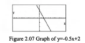
The first example illustrates the illusions encountered when looking at a family of linear equations y=mx+b. To the trained eye or someone who have developed some analytical expectations, the line "move up" as b increases, (or "move down" as b decreases), as in figure 2.03 and figure 2.04. Because of the infinite nature of the line where no discrete points are obvious, the line may appear to move from left to right as the constant term increases (as in figure 2.05 and figure 2.06) or from right to left if the line slope is positive.
Figure 2.03 Graph of y=-0.5x-2 Figure 2.04 Graph of y=-0.5x+2
31
Figure 2.07 Graph of y=-0.5x+2
However, when the x and y-axes are represented on different scales as in figure 2.07, the graph of same equation that appears in figure 2.04 resembles one that belongs to the family of equations represented in figure 2.05 and figure 2.06.
Goldenberg points out that the "zooming in" and "zooming out" operations, which facilitate the user to view "closer to" or "farther from" the graph, are also a source of confusion. Students expect that the shape of the graph will not be affected when they change both axis scales by the same factor. This may be so in the case of straight lines, as shown in figure 2.08 and figure 2.09. However, it appears that the line has moved "closer" to the centre of the window giving the illusion that it has moved higher, thus suggesting that the constant term has changed.
Figure 2.08 Graph of y=-x-2 Figure 2.09 Graph of y=—x-2 in the INIT window when "zoomed out"
With a parabola, it appears that the shape changes when viewed close up as in figure 2.10 and from further away as in figure 2.11. The eyes have been deceived into thinking that the parabola has "narrowed".
X
Figure 2.10 Graph of y=x2-x-1 Figure 2.11 Graph of y=x2-x-1 in the INIT window when "zoomed out"
Figure 2.12 Graphs of y=5x2-2x+1 and y=5x2-2x-2
2.3.2.2 View-windows
Arguably, students' difficulties and misconceptions may be related to the fixed or finite
size of the view-window of the graphing calculator. With graph paper, students can
determine the graphical space (the dimension of the "window") which maintains the
same scale values. However, the graphing calculator has a finite view-window: the
dimension of the window remains the same but what changes is the scale. Students can
miss this fundamental point as the graphing calculator automatically graphs in the
view-window that has been set in the previous activity, which can be the default view-window or
built in window, or some other view-window settings. Cavanagh and Michelmore's
(2000) investigation involving 25 Grade 10-11 students all too clearly points to students'
careless attention to scaling. Only 16% of the students immediately recognised that the
graphs of y=2x+3 and y=-0.5x-2.5 (drawn in the built in "standard window" as shown in
figure 2.13) did not appear at right angles on the screen because of the unequal scaling.
Figure 2.13 Graphs of y=2x+3 and y=-0.5x-2.5 in the "standard window"
Similarly, when given the same graph (y -)- c), one drawn in the default "initial window"
and the other in a window where both the scale and the interval between the tick marks
on the y-axis have been doubled (Figure 2.14), only 8% of the students recognised that
the apparent differences was an artefact of the scaling. The remaining 92% of the
students thought that the second figure represented the line y=0.5x.
iew in ow Xmin 1-10
max :10 scale:1 Ymin 1-10
max :10 Sca e•
IEGEOMBEIEECISTOPM
Cavanagh and Mitchelmore (2000) attribute the difficulty that students have in understanding the scale concept in the graphing calculator environment to students having an absolute understanding of scale rather than a relative understanding. "Absolute" means to interpret scale exclusively as either the measure of the distance between adjacent markings on the axes or as their value, whereas a "relative" interpretation of scale is as the ratio of distance to value. They argue that this might be a result of students' lack of experience of manually drawing graphs with axes that are not scaled equally. They found that students in their study tended to use symmetrically scaled axes marked at regular unit intervals when asked to draw a graph by hand.
The ease with which the graphing calculator allows students to choose the windows, and to readjust in the scales seems to result in some students' unthinking use or to careless treatment of view-windows. In a study by Ward (2000) involving eighteen high school students, he found that students used mainly three strategies to obtain the graph of an equation. 70% of the time students used the "press and pray" strategy: students simply stored the equation and immediately pressed DRAW or GRAPH to display the graph, taking little notice of their window settings. Ward observed that about 16% of the time, students used either the default window or the "standard window", and very few manually set the window using the critical points in the equation. Ward details how the "press and pray" strategy resulted in a "visual conflict" when one student was asked to graph y=3x+400. The student was confused when the graph she drew was not as she predicted. She expected that the line would be quite steep "because the slope is 3". From her previous experience, graphs "always showed up" in the "standard window" and appeared to be quite "steep" (as shown in figure 2.15). She was somewhat baffled when the graph of y=3x+400 did not appear on the screen. She adjusted the viewing window using the y-intercept as a guide resulting in a line that was more "horizontal" as shown in figure 2.16.
Wiew Window Xmin :-10
max :10 scale:1 Ymin :-10
max :450 scale:100
Figure 2.16 Graph of y=3x+400
The problem of the critical use of the default viewing window has been reported in several studies (e.g., Steele, 1993; Ward, 2000; Cavanagh and Mitchelmore, 2000). Cavanagh and Michelmore (2000) report how Grade 10-11 students responded to a task asking them to manually draw a sketch of the graph of y=0.1x2+2x-4. Only 28% of the students sketched a parabola. They all commented that the x2 term indicated that the graph must be a parabola, and zoomed out until they saw the U-shaped graph. The remaining students drew a straight line as their sketch of the quadratic equation with 20% simply copying the straight line directly from the calculator screen using the default viewing window.
2.3.2.3 Tool artefacts
Two aspects are discussed here, the left to right "movement" of plotting and the limitations of the pixel-based screen. The left to right generation of graphs by the graphing calculator can result in a number of misconceptions. Ward (2000) describes how a student who was accustomed to displaying the graph in the default window, interpreted the graph of y=2x3-16x2+12x+6 in the following window setting.
Iew in ow Xmin :-4.7 max :4.7 scale:I Ymin :-3.1
max :3.1
Figure 2.17 The view-window Figure 2.18 The graph of setting y=2x3-16x2+12x+6
only over the parameters in the equation, can mislead students into thinking that the parameters are the variables.
The other confusion .that students have using any graphing technology, including graphing calculators, is related to the physical appearance of the lines on the screen. Each graph is composed of a series of pixels (small rectangular shapes) on the screen, resulting in the line not being represented as smooth. The different patterns of pixels corresponding to different slopes produce different degrees of "jaggedness" on the graphs. The study by Moschkovich et al. (1993) is informative here (although it deals with a computer environment). They found some students misinterpreting the relationship between the jaggedness of the straight lines and the gradient of the line (e.g., compare the graph in figure 2.16 and figure 2.18). They gave an example where students used a graphing program to graph (+2, y=2x+2, y=3x+2,... and were asked to state what they observed. Instead of observing that the lines were increasingly steeper and all passed through (0, 2), they commented on the "insignificant" fact that some of the lines were more jagged than others, according to the magnitude of the coefficient. These observations cause students to see things that were not intended (line jaggedness) and not see things that were intended (point of intersection on the y-axis).