A study on FP Tree Algorithms for Association Rules

!

"!" # $ $"

% & ''' (

A study on FP Tree Algorithms for Association Rules

A. Naresh* Prof Geetha Mary. A

School of Computing Science and Engineering, School of Computing Science and Engineering, VIT University, VIT University,

Vellore-632014, Vellore-632014,

Tamilnadu, INDIA Tamilnadu, INDIA

[email protected] [email protected]

Abstract: A study on the performance of the FP growth method shows that it is efficient and scalable for mining both long and short frequent patterns, and is about an order of magnitude faster than Apriori algorithm. The frequent pattern tree structure, which is an extended prefix tree structure for storing compressed, crucial information about frequent pattern and develop an efficient FP-tree, based mining method. Efficiency of mining is achieved with three techniques: (1) a large database is compressed into a smaller data structure; FP-tree avoids costly, repeated database scans, (2) our FP-tree-based mining avoids the costly generation of a large number of candidate sets, and (3) The FP-tree algorithm avoid repeated scan of database and search database in divide-and-conquer based. We also perform an evaluation study of the hiding algorithms in order to analyze their time complexity and the impact that they have in the original database.

Keywords: Apriori algorithm, FP-tree algorithm, Frequent Pattern, FP-growth

I. INTRODUCTION

Frequent pattern mining is an important part in the data mining task. It is the fastest and most popular for finding the frequent item sets in the FP-growth algorithm [7]. It is based on a prefix tree representation of a given database called an FP-tree, which can save the considerable amount of memory for storing the transaction. The main basic idea of the FP-growth algorithm is the recursive elimination schema: in the preprocessing step we can eliminate all the non frequent items from the transaction. The set of frequent items is sorted and arranged in the order of descending support count. We can also reduce the database scan the item sets found in the recursion share the deleted items as a prefix. Let I be the set of items and D be the set of transaction, where each transaction T is a set of

items such that T I. for any x I, we say that a

transaction T contains X if X T is called an item set [2]. The count of an itemset X is the number of transactions in D that contain X. The support of an itemset X is the proportion of transactions in D that contain X. In order to solve this problem, we proposed the FP-growth [6]algorithm based on FP_tree that used the compressed FP_tree structure to store the frequent patterns and did not generate candidate sets. Such as suffix Span [4], Prefix Span [5] based on FP-growth approach can mine all frequent item set in database. Apriori employs an iterative approach known as level wise search, where k –item sets are used to explore (K+1)-item sets [8]. The frequent pattern growth which adopts a divide and conquers strategy as follows: compress the database representing frequent items into a frequent pattern tree, or FP-tree but retain the item set association information, and then divide such a compressed database into a set of conditional database (a special kind of projected database), each associated with one frequent item, and mine each such database separately.

II. COMPRATIVESTUDY

The FP-tree stores a single item at each node and includes additional links to facilitate Preprocessing. Construction process begins with an initial pass to count support for the single items [1]. The Efficient fast algorithms for mining frequent patterns item sets [2] are crucial for mining association rules and for other data mining tasks. In this method the frequent item sets have been implemented using a prefix-tree structure, known as an FP-tree, for storing compressed information about frequent item sets. Recently most of the mining frequent patterns focus on improving the efficiency of frequent item sets generations [3], but the input output cost of database scanning has been a bottle-neck problem in data mining. Many algorithms are recently based on Apriori and FP-tree, and FP-growth algorithm based on FP-tree is more efficient than Apriori because the candidates are not generated. First scan the database only once for generating equivalence classes of each item. Second, delete the non-frequent items and rewrite the equivalence classes of the frequent items, and then construct the FP-tree. It’s made of a root node labeled as null and child nodes consisting of the item-name, support and node link. Moreover, database scans are made only twice [8]. First database scan is done to create frequent item set and sorted in the order of descending support count in the header table. Secondly, frequent items are extracted. Afterwards, sort these items then frequent items are inserted to the tree.

.

III. THEAPRIORIALGORITHM

prior knowledge of frequent item sets properties. It is an iterative approach known as a level wise search, where K item sets are used to explore (K+1) item sets. First the set of frequent 1 item sets is found this is denoted as L1. L1 is used to find L2. The set of frequent 2 item sets which is used to find L3. So on more frequent K item sets can be found. Finding of each Lk requires one full scan of the database. Improving the efficiency of the level wise generation of frequent item sets an important property called the Apriori property used to reduce search space. If an item set I does not satisfy the minimum support threshold, min_sup; then I is not frequent, p (I) < min_sup. If an item A is added to the item set I, then the resulting item set (IUA), cant occur more therefore IUA is not frequent with P(IUA)< min_sup. Apriori property used in the algorithm is a two step process is followed consist of join and prune action. In join component LK-1 is joined with Lk-1 to generate potential candidates. Prune component apriori property to remove candidates that have a subset that is not frequent.

Table1: an example the transaction database and min_sup=2

The Apriori heuristic can prune candidates dramatically. Based on this property, a fast frequent item set mining algorithm, called Apriori, was developed. It is illustration in the following example.

Example 1 (Apriori) let’s give an example with five transactions DB and support threshold is set to 3 in Table 1. The process of Apriori Algorithm to find the complete frequent patterns in DB as follows, Figure 1 illustrates this process.

1. Scan DB once to generate length-1 frequent item sets, labeled as F1. In this example, they are {1, 2, 3, 5}.

2. Generate the set of length-2 candidates, denoted as C2 from F1.

3. Scan DB once more to count the support of each item set in C2. All item sets that turn out to be frequent in C2 are inserted into F2. In this example, F2 contains {(1; 2); (1; 3); (1; 5); (2; 3); (2; 5); (3; 5)}.

4. Then, we form the set of length-3 candidates from F2 and frequent 3-itemsets

F3 from C3. The similar process goes on until no candidates can be derived or no candidate is frequent.

Apriori performs a BFS by iteratively obtaining candidate item sets of size (k+1) from frequent item sets of size k, and check their corresponding occurrence frequencies in the database. Many variants that improve Apriori have been proposed by reducing the number of candidates further, the number of transactions to be scanned, or the number of database scans, the process is still expensive as it is tedious to repeatedly scan the database and check a large set of candidates by pattern matching, which is particularly true if a long pattern exists. In short, the bottleneck for Apriori-like methods is the candidate-generation-and-testoperation.

Figure.1 The Apriori algorithm - example

IV. FREQUENT-PATTERN TREE: DESIGN AND

CONSTRUCTION

Let I ={a,b,c……s} be a set of items, and a transaction database DB={100,200…..600}, where Ti (i = [1 . . . n]) is a transaction which contains a set of items in I . The support (or occurrence frequency) of a pattern A, where A is a set of items, is the number of transactions containing A in DB. A pattern A is frequent if A’s support is no less than a predefined minimum support threshold, . Given a transaction database DB and a minimum support threshold , the problem of finding the complete set of frequent patterns is called the frequent-pattern mining problem [9].

A. Frequent-pattern tree

To design a compact data structure for efficient frequent-pattern mining, let’s first examine an example. Example.2: Let the transaction database, DB, be the first two columns of Table 2, and the Minimum support threshold be 3 (i.e., = 3).

A compact data structure can be designed based on the following observations:

1. The frequent items will play a role in the frequent-pattern mining, it is necessary to perform one scan of transaction database DB to identify the set of frequent items.

2. The set of frequent items of each transaction can be stored in some compact structure, it may need to repeatedly scan the database and check a large set of candidates by pattern matching.

3. If multiple transactions share a set of frequent items is sorted in the order of descending support count.

.

TID Item

100 1 3 4

200 2 3 5

300 1 2 3 5

4. If two transactions share a common prefix, according to some sorted order of frequent items, the shared parts can be merged using one prefix structure as long as the count is registered properly. If the frequent items are sorted in their frequency descending order, there are better chances that more prefix strings can be shared.

First, scan of the database is the same as Apriori, which derives a set of frequent items, {(f: 4), (c: 4), (a: 3), (b: 3), (m: 3), (p: 3)} (the number after “:” indicates the support), and there support counts (frequency). The set of frequent items is sorted in the order of descending support count. Second, create the root of the tree, labeled with “null”. Scan database D a second time. The items in each transaction are processed in L order and a branch is created for each transaction.

1. The scan of the first transaction, “T100: f, a, c, d, g, i, m, p”. Which contains five items (f, c, a, m, p) in L order. 2. For the second transaction, T200, contains the items a, b, c, f, l, m, o in L order, which would result in branch since its frequent item list {f, c, a, b, m} shares a common prefix {f, c, a} with the existing path {f, c, a, m, p}, the count of each node along the prefix is incremented by 1, and one new node (b:1) is created and linked as a child of (a:2) and another new node (m:1) is created and linked as the child of (b:1).

3. For the third transaction, since its frequent item list { f, b} shares only the node { f } with the f -prefix sub tree, f ’s count is incremented by 1, and a new node (b:1) is created and linked as a child of ( f :3).

4. The scan of the fourth transaction leads to the construction of the second branch of the tree, {(c: 1), (b: 1), (p: 1)}.

5. For the last transaction, since its frequent item list {f, c, a, m, p} is identical to the path is shared with the count of each node along the path incremented by 1.

To facilitate tree traversal, an item header table is built in which each item points to its first occurrence in the tree via a chain node-link. After scanning all the transactions, the tree, together with the associated node-links, are shown in figure.2:

Figure.2 FP-tree the minimum support= 3

Figure.3 FP-tree to Conditional Pattern Base

• Starting at the frequent header table in the FP-tree.

• Traverse the FP-tree by following the link of each

frequent item.

• Accumulate all of transformed prefix paths of that

item to form a conditional pattern base.

• Construct the FP-tree for the frequent items of the

pattern base.

Algorithm 2 (FP-tree construction):

1. Scan the transaction database DB once. Collect, the set of frequent items F, and their supports. Sort F in support descending order as L, the list of frequent items.

2. Create the root of an FP-tree, and label it as “null”. For each transaction Trans in DB do the following. Select the frequent items in Transaction according to the order of L. Let the sorted frequent-item list in Trans be [p | P], where p is the first element and P is the remaining list.

V. ANALYSIS

The efficient data structure for mining frequent patterns is FP tree [10], [11] have been used and its fluctuations used for “iceberg” data computation [12]. The most important work is a novel technique that uses a special data structure, called an FP array, and it is used to improve the performance of the algorithms operating on FP-trees. The FP array technique drastically speeds up the FP-growth method on sparse data sets and it now scan each FP-tree only once for each recursive call proceed from it. This technique is then applied to the other algorithm FP max for mining maximal frequent item sets in the data base. In FP max the technique for checking if a frequent item set is maximal is also introduced, for which a variant of the FP-tree structure MFI-FP-tree, is used. For mining closed frequent item sets, the design of an algorithm FP close which uses another variant of the FP-tree structure, called a CFI-tree, for Checking the closeness of frequent item sets [13].

VI TREE PARTITION ALGORITHM

A. Master/Slave Model

In the multi-thread environments, we make one thread as the master thread, and the remaining threads as slave threads [14]. The master thread’s task is for to load each line of transaction from the database and distribute it to each slave threads. Each slave thread has its own transaction queue. It gets a transaction from the queue each time the master thread put one transaction into it, and disposes the transaction to build the tree. Thus the master thread is a producer, which produces transactions for each slave thread to consume. This model makes it possible for master thread to do some preliminary measures of the transaction before receiving at the slave thread. According to the results of the preliminary measures, the master thread can also decide to which slave thread the transaction should be sent.

B. Content based tree partition

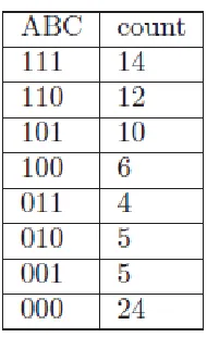
The most important point is to partition the tree equally so that each thread can get equal workload and equal amount of transactions to process. In a database the data contains 8 items: A, B, C…., H where A, B and C are the first three most frequent items. Assume the partitioning of all transactions according to the content of first N most frequent items Here we set N = 3 for simplicity and the transactions are partitioned into 2^3 = 8 chunks according to items “A”, “B” and “C” See Table 3 for an example of the distribution chunks. e.g. 110 means the chunk contain transactions all have items “A” and “B”, but not “C”. If there are two threads available, i.e. need to group the chunks into two groups, a heuristic search algorithm can be employed to group the 8 chunks into two groups, and make each group contain equal number of transactions. The result can be {111, 110, 101, 011} and {100, 101, 001, 000}, each group contains 40 transactions. Two sub-branches circled with red dashed line are the group assigned to thread 1, and two other sub-branches circled with blue solid line are the group assigned to thread 2.

Figure.5 Content based tree partition and grouping

Table 3: Transaction Distributionby Contents

Advantage of FP-growth Algorithm

The major advantages of FP-Growth algorithm is,

• Uses compact data structure

• Eliminates repeated database scan

FP-growth is a faster than other association mining algorithms and is also faster than tree- Researching. The algorithm reduces the total number of candidate item sets by producing a compressed version of the database in terms of an FP-tree.

The algorithm consists of two steps:

• Compresses a large database into a compact, Frequent-Pattern tree(FP-tree) structure

• Develop an efficient, frequent pattern mining

method (FP-growth)

A divide-and-conquer methodology: decompose mining

tasks larger ones to smaller ones and avoid candidate generation.

Advantage of FP-tree Structure

The most significant advantage of the FP-tree structure is the algorithm scans the tree only twice.

Completeness:

- The FP-tree contains all the information related to frequent pattern mining.

– The height of the tree is bounded by the maximum number of items in a transaction.

Three major steps performed are starting the processing from the end of list L:

Construct conditional pattern base for each item in the header table.

Construct conditional FP-tree from each conditional pattern base.

Recursively mine conditional FP-trees and grow frequent patterns obtained. If the conditional FP-tree contains a single path, simply enumerate all the patterns.

VII. CONCLUSION

In a novel data structure, frequent pattern tree (FP-tree), for storing and compressed of crucial information about frequent patterns, and developed a pattern growth method, for efficient mining of frequent patterns in large databases. There are several advantages of FP-growthover other approaches: (1) it may need to repeatedly scan the database and check a large set of candidates by pattern matching. (2) It applies a pattern growth method which avoids costly candidate generation. The major operations of mining are count accumulation and prefix path count adjustment, which are usually much less costly than candidate generation and pattern matching operations performed in most Apriori algorithms. (3) It applies a partitioning-based divide-and-conquer method which dramatically reduces the size of the subsequent conditional pattern bases and conditional FP-tree. Several other optimization techniques, including direct pattern generation for single tree-path and employing the least frequent events as suffix, also contribute to the efficiency of the method.

VIII.REFERENCES

[1] Christian Borgelt,” An Implementation Of the FP growth Algorithm”, ACM Proceedings, OSDM’05-Knowledge Discovery and Data Mining, 2005

[2] Go Sta Grahne, and Jianfeizhu,”Fast Algorithms for Frequent Item set Mining using FP-Trees” Transactions On Knowledge and Data Engineering, VOL. 17, No10,October 2005.

[3] Jiao-Minliu, Shengguo, Zhen- Zhou Wang,” A Fast Algorithm for Constructing FP-Tree” Proceedings of The Sixth International Conference on Machine

Learning and Cybernetics,Hong Kong, 19-22 August 2007.

[4] J.Han, J.Pei, and B.Mortazavi, “Free-Span: Frequent Pattern-projected Sequential pattern Mining”, of the 6th ACM Sigkd Int.Conf. on Knowledge Discovery and Data Mining, Boston, New York, ACM Press, pp. 355-359, 2000.

[5] J.Pei, J.Han, and H.Pinto, “Prefix Span: Mining Sequential Patterns Efficiently by Prefix-projected Pattern Growth”, of the 17th Int. Conf. on Data Engineering, Heidelberg, Germany, Los Alamitos, CA, Computer Society Press, pp. 215-224, 2001.

[6] J.Han, J. Pen, and Y.Yin, “Mining Frequent Patterns without Candidate Generation: a Frequent-Pattern tree Approach”, Proc. ACM-SIMOD Int., pp.53-87, 2004. [7] J.Han, H.Pei, and Y.Yin,” Mining Frequent

Patternswithout Candidate Generation” In: Proc. Conf. on theManagement of Data. ACM Press, New York, NY,USA 2000.

[8] Jiayi Zhou, Kun-Ming Yu,” Balanced Tidset-based Parallel FP-tree Algorithm for the Frequent Pattern Mining on Grid System”, Fourth International Conference Semantics, Knowledge and Grid, IEEE Computer Society, 2008, Pages 103-108.

[9] Jia Weihan, “Mining Frequent Patterns without Candidate Generation: A Frequent-Pattern Tree Approach” Data Mining and Knowledge Discovery, Kluwer Academic Publishers. Vol. 8, pp.53–87, 2004. [10] J.Han, J. Pei, and Y. Yin, “Mining Frequent Patterns

without Candidate Generation,” Proc. ACM-Sigmod Int.l Conf. Management of Data, pp. 1-12, May 2000. [11] J. Han, J. Wang, Y. Lu, and P.Tzvetkov, “Mining

Top-K Frequent Closed Patterns without Minimum Support,” Proc. Int’l Conf. Data Mining, pp. 211-218, Dec. 2002.

[12] D. Xin, J. Han, X. Li, and B.W. Wah, “Star-Cubing: Computing Iceberg Cubes by Top down and Bottom-Up Integration”, VLDB '03 Proceedings of The 29th international Conference on Very large data bases Volume 29, pp. 476-487, Sept. 2003.

[13] B. Goethals, and M.J. Zaki, Proc. ICDM Workshop “Frequent Item set Mining Implementations“CEUR Workshop Proc., vol. 80, Nov. 2003 Vol-90.