Feature Selection and Blind Source Separation in an EEG-Based Brain-Computer Interface

(1)

Feature Selection and Blind Source Separation

in an EEG-Based Brain-Computer Interface

David A. Peterson

Department of Computer Science, Center for Biomedical Research in Music, Molecular, Cellular, and Integrative Neurosciences Program, and Department of Psychology, Colorado State University, Fort Collins, CO 80523, USA

Email:[email protected]

James N. Knight

Department of Computer Science, Colorado State University, Fort Collins, CO 80523, USA Email:[email protected]

Michael J. Kirby

Department of Mathematics, Colorado State University, Fort Collins, CO 80523, USA Email:[email protected]

Charles W. Anderson

Department of Computer Science and Molecular, Cellular, and Integrative Neurosciences Program, Colorado State University, Fort Collins, CO 80523, USA

Michael H. Thaut

Center for Biomedical Research in Music and Molecular, Cellular, and Integrative Neurosciences Program, Colorado State University, Fort Collins, CO 80523, USA

Received 1 February 2004; Revised 14 March 2005

Most EEG-based BCI systems make use of well-studied patterns of brain activity. However, those systems involve tasks that indi-rectly map to simple binary commands such as “yes” or “no” or require many weeks of biofeedback training. We hypothesized that signal processing and machine learning methods can be used to discriminate EEG in a direct “yes”/“no” BCI from a single session. Blind source separation (BSS) and spectral transformations of the EEG produced a 180-dimensional feature space. We used a modified genetic algorithm (GA) wrapped around a support vector machine (SVM) classifier to search the space of feature subsets. The GA-based search found feature subsets that outperform full feature sets and random feature subsets. Also, BSS trans-formations of the EEG outperformed the original time series, particularly in conjunction with a subset search of both spaces. The results suggest that BSS and feature selection can be used to improve the performance of even a “direct,” single-session BCI.

Keywords and phrases:electroencephalogram, brain-computer interface, feature selection, independent components analysis,

support vector machine, genetic algorithm.

1. INTRODUCTION

1.1. EEG-based brain-computer interfaces

There is a fast-growing research and development eﬀort un-derway to implement brain-computer interfaces (BCI) using

This is an open access article distributed under the Creative Commons Attribution License, which permits unrestricted use, distribution, and reproduction in any medium, provided the original work is properly cited.

the electroencephalogram (EEG) [52]. The overall goal is to provide people with a new channel for communication with the external environment. This is particularly important for patients who are in a “locked-in” state in which conventional motor output channels are compromised.

(2)

system. For example, subjects may be required to imagine left- or right-hand movement in order to use the BCI [3,37,

39]. If they want to use the BCI to respond yes/no to ques-tions, they have to remember that left-hand imagined ment corresponds to “yes,” and right-hand imagined move-ment corresponds to “no.” Other BCI research requires ex-tensive subject biofeedback training in order for the subject to gain some degree of voluntary influence over EEG features such as slow cortical potentials [5] or 8–12 Hz rhythms [53]. For both the imagined movement and biofeedback scenarios, the mapping between what the subject does and the eﬀect on the BCI is indirect. In the latter case, a single session is insuf-ficient and the subject must undergo many weeks or months of training sessions.

A more direct approach would simply have the sub-ject imagine “yes” or “no” and would not require extensive biofeedback training. While imagined movement and bidi-rectional influence over time- and frequency-domain ampli-tude can be readily detected and used as control signals in a BCI, the EEG activity associated with complex cognitive tasks such as imagining diﬀerent words is much more poorly understood. Can advances in signal processing and pat-tern recognition methods enable us to distinguish whether a subject is imagining “yes” or “no” by the simultaneously recorded EEG? Furthermore, can that distinction be learned in a single recording session?

1.2. The EEG feature space

The EEG measures the scalp-projected electrical activity of the brain with millisecond resolution at up to over 200 elec-trode locations. Although most EEG-based BCI research uses far fewer electrodes, research into the role of the specific to-pographic distribution of the electrodes [54] suggests that dense electrode arrays may standardize and enhance the sys-tem’s performance. Furthermore, advances in electrode and cap technology have made the time required to apply over 200 electrodes reasonable even for BCI patients. EEG anal-yses, including much of the EEG-based BCI research, make extensive use of the signals’ corresponding frequency spec-trum. The spectrum is usually divided into five canonical fre-quency bands. Thus, if one considers the power in each of these bands for each of 200 electrodes, each trial is described by 1000 “features.” If interelectrode features such as cross-correlation or coherence are considered, this number grows combinatorially. As in many such problems, a subset of fea-tures will often lead to better dissociation between trial types than the full set of features. However, the number of unique feature subsets forNfeatures is 2N_{, a space that cannot be} ex-haustively explored forNgreater than about 25. This is but one reason why most EEG research uses only a very small number of features. A significant number of features are dis-carded, including features that might significantly improve the accuracy with which the signals can be classified.

1.3. Blind source separation of EEG

Given a set of observations, in our case a set of time series, blind source separation (BSS) methods such as independent

component analysis (ICA) [22] attempt to find a (usually linear) transformation of the observations that results in a set of independent observations. Infomax [4] is an imple-mentation of ICA that searches for a transformation that maximizes the information between the observations and the transformed signals. Bell and Sejnowski showed that a trans-formation maximizing the intrans-formation is, in many cases, a good approximation to the transformation resulting in in-dependent signals. ICA has been used extensively in analyses of brain imaging data, including EEG [26,34], magnetoen-cephalogram (MEG) [47,49], and functional magnetic res-onance imaging (FMRI) [26]. Assumptions about how inde-pendent brain sources are mixed and map to the recorded scalp electrodes, and the corresponding relevance for BSS methods, are discussed extensively in [27].

Maximum noise fraction (MNF) is an alternative BSS ap-proach for transforming the raw EEG data. It was initially introduced in the context of denoising multispectral satellite data [14]. Subsequently it has been extended to the denois-ing of time-series [1] and it has been compared to principal components analysis and canonical correlation analysis in a BCI [2]. The basis of the MNF subspace approach is to con-struct a set of basis vectors that optimize the amount of noise (or, equivalently, signal) captured. Specifically, the maximum noise fraction basis maximizes the noise-to-signal (as well as the signal-to-noise) ratio of the transformed signal. Thus, the optimization criterion is based on the ratio of second-order statistical quantities. Furthermore, unlike ICA, the basis vec-tors have a natural ordering based on the signal-to-noise ra-tio. MNF is similar to the second-order blind identification (SOBI) algorithm and requires that the signals have diﬀerent autocovariance structures. The requirement exists because of the second-order nature of the algorithm.

The relationship of MNF to ICA is a consequence of the fact that they both provide methods for solving the BSS prob-lem [1,21]. Initial results for the application of MNF to the analysis of EEG time-series demonstrated MNF was simulta-neously eﬀective at eliminating noise and extracting what ap-peared to be observable phenomenon such as eye blinks and line noise [28,29]. It is interesting that ICA and MNF per-form similarly given their disparate per-formulations. This sug-gests that under appropriate assumptions (see [1,21,28]) the mutual information criterion and the signal-to-noise ratio can be related quantities. However, in the instance that sig-nals of interest are mixed such that they share the same sub-space, the MNF approach provides a representation for the mixed and unmixed subspaces.

1.4. Classification and the feature selection problem

(3)

also been successfully employed in EEG-based BCI research [6,12,32,56]. In contrast to competing nonlinear classifiers such as multilayer perceptrons, SVMs often exhibit higher classification accuracy, are not susceptible to local optima, and can be trained much faster. Because we seek feature sub-sets that maximize classification accuracy, the feature subset search needs to be driven by how well the data can be clas-sified using the corresponding feature subsets, the so-called “wrapper” approach to feature selection [30]. Thus the speed characteristic of SVMs is particularly important because we will train and test the classifiers for every feature subset we evaluate.

Our prior research with EEG datasets from a cognitive BCI [2] and movement prediction BCI [12] demonstrated the benefit of feature selection for small and large feature spaces, respectively. There are many ways to implement the feature selection search [7,16,42]. One logical choice is a genetic algorithm (GA) [13,20]. GAs provide a stochastic global search of the feature subset space, evaluating many points in the space in parallel. A population of feature subsets is evolved using crossover and mutation operations akin to natural selection. The evolution is guided by how well feature subsets can classify the trials. GAs have been successfully em-ployed for feature selection in a wide variety of applications [15,51,55] including EEG-based BCI research [12,56]. GAs often exhibit superior performance in domains with many features [46], do not get trapped in local optima as with gra-dient techniques, and make no assumptions about feature in-teractions or the lack thereof.

In summary, this paper evaluates a feature selection sys-tem for classifying trials in a novel, challenging BCI using spectral features from the original, and two BSS transforma-tions of, scalp recorded EEG. We hypothesized (1) that clas-sification accuracy would be higher for the feature subsets found by the GA than for full feature sets and random feature subsets and (2) that the power spectra of the BSS transforma-tions would provide feature subsets with higher classification accuracy than the power spectra of the original signals.

2. METHODS

2.1. Subjects

The subjects were 34 healthy, right-handed fully informed consenting volunteers with no history of neurological or psy-chiatric conditions. The present paper is based on data from eight of the subjects who met certain criteria for behavioral measures and details of the EEG recording procedure. Specif-ically, we selected eight subjects that wore caps with physi-cally linked mastoids for the reference. Other subjects wore a cap with mastoids digitally linked for the reference. Although the diﬀerence between physically and digitally linked mas-toid reference is minor, it can be nontrivial depending on the relative impedances at the two mastoid electrodes [36]. Thus, to eliminate the possibility that the slight diﬀerence in caps could influence the questions at hand, we elected to consider only those subjects wearing the cap with physi-cally linked mastoids. We also considered only those subjects

0 0.75 1.5 2.5 3 s EEG

<Visualize>· · ·(100 trials) No

Yes Visual display

Figure 1:BCI task timeline.Subjects were asked to visualize the most recently presented word until the next word is displayed. The period of simultaneously recorded EEG used for subsequent anal-ysis was 1000 milliseconds long beginning 750 milliseconds after display oﬀset and 500 milliseconds before the next display onset.

that exhibited reasonable inter-response intervals and a rea-sonably even distribution of “yes”/“no” responses in a sep-arate, voluntarily decided premotor visualization version of the task (described in a separate forthcoming manuscript). The subjects were selected on these criteria only, before their EEG data was reviewed. The eight subjects were 19 +/−1 years of age and included five females.

2.2. BCI experiment procedure

On each of 100 trials subjects were shown one of the words “yes” or “no” on a computer display for 750 milliseconds and were instructed to visualize the word until the next word is displayed (seeFigure 1). There were 50 “yes” trials and 50 “no” trials presented in random order with a maximum of three of the same stimulus in a row. Because in subsequent analyses we planned to ignore the first two trials due to ex-periment start-up transients, the first two trials were required to include exactly one of each type.

2.3. EEG recording and feature composition

The EEG was continuously recorded with a 32-electrode cap (QuikCap, Neuroscan, Inc.), pass band of 1–100 Hz, and sampled at 1 kHz. Although much higher than the 200 Hz required by Nyquist, we typically sample at 1 kHz for the mere convenience that in subsequent time-domain analyses and plots, samples are equivalent to milliseconds. Electrodes FC4 and FCZ were excluded because of sporadic techni-cal problems with the corresponding channels in the ampli-fier. The remaining 30 electrodes used in subsequent analy-sis included bipolar VEOG and HEOG electrodes commonly used to monitor blinks and eye movement artifacts. All other electrodes were referenced to physically linked mastoids. We did not employ any artifact removal or mitigation in the present study, as we sought to measure performance with-out the added help or complexity of artifact mitigation tech-niques.

(4)

software1_[₁₀_{]. The EEGLAB software first spheres the data,}

which decorrelates the channels. This simplifies the ICA pro-cedure to finding a rotation matrix which has fewer degrees of freedom [23]. Except for the convergence criteria, all of the default parameter values for EEGLAB’s Infomax algorithm were used. Initially, extended Infomax, which allows for sub-Gaussian as well as super-sub-Gaussian source distributions, was used. No sub-Gaussian sources were extracted on the first two subjects so the standard Infomax approach was used on all of the subject data. An initial transformation matrix was found with a tolerance of 0.1. The algorithm was then rerun with this transformation matrix and a tolerance of 0.001.

To investigate whether comparing Infomax ICA and the MNF method would be of empirical value, a simple test was performed on the data set for several subjects. Both trans-forms were applied to each subject’s data and the resulting components were compared. The cross-correlation for all Infomax-MNF component pairs was computed, and the op-timal matching was found. This matching paired the com-ponents so that the maximal cross-correlation was achieved. Had the components produced been the same, the cross-correlation measure would have been 100%. Cross correla-tions of 60–70% were found in the tests performed, and so we decided the two transforms were suﬃciently dissimilar to warrant the evaluation of both in the study.

Each of the original, Infomax, and MNF-transformed data were “epoched” such that the one-second period begin-ning 750 milliseconds after stimulus oﬀset was used for sub-sequent analysis. Because iconic memory is generally thought to last about 500 milliseconds, this choice of temporal win-dow should minimize the influence of iconic memory and place relatively more weight on active visualization processes. We then computed spectral power for each channel (com-ponent) and each trial (epoch) using Welch’s periodogram method that uses the average spectra from overlapping win-dows of the epoch. We computed averaged spectral power in the delta (2–4), theta (4–8), lower alpha (8–10), upper alpha (10–12), beta (12–35), and gamma (35–50 Hz) frequency bands. Thus, the full feature set contains 30 electrodes×6 spectral bands each for a total of 180 features. The first and second trials were excluded to reduce the transient eﬀects of the start of the task. Thus, all subsequent analyses use 49 tri-als of each type (“yes,” “no”) for each subject. All reported results are for individual subjects.

2.4. Classification

In the present report, we sought subsets from a very large fea-ture set that would maximize our ability to distinguish “yes” from “no” trials. The distinction was tested with a support vector machine (SVM) classifier and an oversampled variant of 10-fold cross-validation.

As discussed in the introduction, we chose a support vec-tor machine (SVM) classifier because of its record of very

1_{Available from the Swartz Center for Computational} Neuro-science, University of California, San Diego, http://www.sccn.ucsd.edu/ eeglab/index.html.

good classification performance in challenging problem do-mains and its speed of training. We used a soft margin SVM2

with a radial basis function (RBF) kernel withγ =0.1. The SVM was trained with regularization parameter υ = 0.8, which places an upper bound on the fraction of error exam-ples and lower bound on the fraction of support vectors [44]. Given m training examplesX{x1,. . .,xm} ⊆ RN and their corresponding class labelsY = {y1,. . .,ym} ⊆ {−1, 1}, the SVM training produces nonnegative Lagrange multipliersαi that form a linear decision boundary:

f(x)= m

i=1

yiαik

x,xi

(1)

in the feature space3_{defined by the Gaussian kernel (of width}

inversely proportional toγ):

kx,xi

=exp−γx−xi2

. (2)

On each feature subset evaluation, we trained and tested the SVM on one full run of stratified 10-fold cross-validation, randomly selecting with replacement 10% of the trials on each fold for testing.

2.5. Feature selection

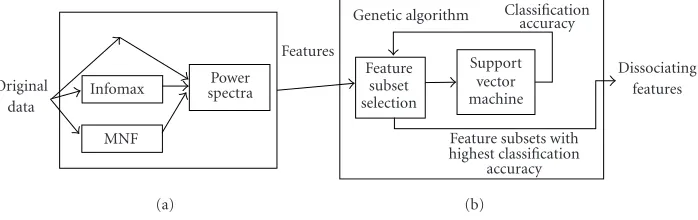
We used a genetic algorithm (GA) to search the space of fea-ture subsets in a “wrapper” fashion (seeFigure 2). Individu-als in the GA were simply bit strings of length 180, with a 1 indicating the feature was included in the subset and 0 indi-cating it was not. Our Matlab GA implementation was based on Goldberg’s original simple GA [13], using roulette-wheel selection and 1-point crossover. We used conventional values for the probability of crossover (0.6) and that of mutation (1/(4∗D), whereD=number of features, or 0.0014). We evolved a population of 200 individuals over 50 generations. Each individual’s “fitness” measure was determined by the corresponding subset’s mean classification accuracy.

We instrumented the GA with a mechanism for main-taining information about the cumulative population, that is, all individuals evaluated thus far. Thus, individuals that were evaluated more than once develop a list of evaluation measures (classification accuracies). This took advantage of the inherent “resampling” that occurs in the GA because rela-tively “fit” individuals are more likely to live on and be reeval-uated in later generations than “unfit” individuals. Such re-sampling, with diﬀerent partitions of the trials into train-ing/test sets on each new evaluation, reduces the risk of fitting due to selection bias. The empirical eﬀect of this over-sampled variant of cross-validation and its role in feature se-lection search is illustrated in the first part ofSection 3. All

2_{The SVM was implemented with version 3}_._{00 of the OSU SVM} Tool-box for Matlab [33], which is based on version 2.33 of Dr. Chih-Jen Lin’s LIBSVM.

(5)

Original data

Infomax

MNF

Power spectra

Features

Genetic algorithm

Feature subset selection

Support vector machine

Classification accuracy

Feature subsets with highest classification

accuracy

Dissociating features

(a) (b)

Figure2:Feature selection system architecture.Three feature “families” were composed with parallel and/or series execution of signal trans-formations. Feature subsets are then evaluated with a support vector machine (SVM) classifier and the space of possible feature subsets searched by a genetic algorithm (GA) guided by the classification accuracy of the feature subsets. (a) Feature composition. (b) Feature selection. (Adapted from [12, Figure 1].)

subsequent reports of classification accuracy use the mean of the 10 best feature subsets that were subjected to at least five “sample evaluations” each.

3. RESULTS

3.1. Fitness evolution and overfitting at the feature selection level

Figure 3shows how the fitness of feature subsets evolves over generations of the GA. In these and subsequent figures, the “chance” level of classification accuracy (50%) is shown with a dotted line. Note that even at the first generation of ran-domly selected feature subsets, the average performance of the population is slightly above chance at 54%. This sug-gests that, on average, randomly chosen feature subsets pro-vide some small discriminatory information to the classifier. The approximately 70% accuracy maximum mean fitness in the first generation of the GA represents a single “sampling” of the 10-fold cross-validation. Thus, there exists a set of 10 randomly chosen training/test trial partitions for which one of the 200 initial, randomly chosen feature subsets gave 70% classification accuracy. However, such results need to be assessed with caution, as illustrated in the right panel of

Figure 3. Further “sampling” for a given feature subset (i.e., repetitions of a full 10-fold cross-validation) gives a more ac-curate picture of that feature subset’s ability to dissociate the “yes” and “no” trials.

3.2. The benefit of feature selection

Figure 4shows how classification accuracy is improved when comparing feature subsets selected by the GA with full fea-ture sets. For every BSS transformation (original, Infomax, and MNF) every subject’s “yes”/“no” visualizations are bet-ter distinguished with feature subsets than with the whole feature set.

3.3. The benefit of BSS transformations

Figure 5 shows for each subject how the classification ac-curacies compare for the original signals and the two BSS

transformations. For every subject, at least one of the BSS transformations leads to better classification accuracy than the original signals. Spectra of Infomax and MNF transfor-mations performed statistically significantly better than the spectra of the original signals for every subject except sub-ject 1 and MNF for subsub-ject 5 (Wilcoxon rank-sum test, alpha = 0.05). The relative performance of the three transforma-tions does not appear to be an artifact of random processes in the GA because it holds across two entirely separate runs of the GA.

3.4. Intersubject variability in good feature subsets

Figure 6 shows the features selected for the feature subsets that provided the highest classification accuracy. For both subjects, the features include a diverse mix of electrodes and frequency bands. Although spatial trends emerge (e.g., the full power spectrum was included for electrodes FC3 and CZ), no single frequency band was included across all elec-trodes. Also, there appears to be some consistency between subjects in terms of the selected features. Subject 1’s best fea-ture subset included 106 feafea-tures and subject 6’s best feafea-ture subset included 91 features. The two subjects’ best subsets had 57 features in common, including broadband features from central and left frontocentral scalp regions.

3.5. Feature values corresponding to the “yes” and “no” trials

(6)

0 10 20 30 40 50 Generation

40 45 50 55 60 65 70 75 80

Classification

ac

cur

acy

(%)

Max Avg

(a)

2 4 6 8 10

Number of samples 40

45 50 55 60 65 70 75 80

Classification

ac

cur

acy

(%)

(b)

Figure3:Feature subset evolution and overfitting.(a) Mean fitness of all individuals in the cumulative population as of that generation; “avg” is the average and “max” the maximum mean fitness. Data shown is for subject 6, Infomax transformation. Note that the maximum mean fitness in the cumulative population does not monotonically increase because repeated sampling of a particularly fit individual may reduce that individual’s mean fitness value (see (b)). (b) Mean fitness of the best individual in the population for each of several diﬀerent “sampling” values. Each “sample” is the mean classification accuracy from a full 10-fold cross-validation run, which uses 10 randomly selected train/test partitions of the trials for that subject. The generally decreasing function reflects overfitting at the feature selection level, whereby so many feature subset evaluations occur that the system finds train/test partitions of the trials that lead to higher-than-average fitness for a specific feature subset. Additional sampling of how well that feature subset classifies the data increases confidence that the oversampled result is not simply due to 10 fortuitous partitions of the trials.

4. DISCUSSION

4.1. Feature selection in the EEG-based BCI

We implemented a feature selection system for optimizing classification in a novel, “direct” EEG-based BCI. For all three representations of the signals (original, Infomax, and MNF) and for all subjects, the GA-based search of the feature sub-set space leads to higher classification rates than both the full feature sets and randomly selected subsets. This indi-cates that choosing feature subsets can improve correspond-ing classification in an EEG-based BCI. This also indicates that it is not simply smaller feature sets that lead to improved classification, but the selection of specific “good” feature sub-sets. Also, classification accuracy improves over generations of the GA’s feature subset search, indicating that the GA’s it-erative search process leads to improved solutions. We ran the GA for over 700 generations for one subject’s Infomax

data, and the resultant feature subsets demonstrated more than a 14% increase in classification accuracy over that ob-tained after just 50 generations. Although this suggests an extensive search of the feature subset space may be benefi-cial, the roughly one week of additional computational time may be inappropriate for some BCI research settings.

(7)

All Subset 40

45 50 55 60 65 70

Classification

ac

cur

acy

(%)

(a)

All Subset 40

45 50 55 60 65 70

Classification

ac

cur

acy

(%)

(b)

All Subset 40

45 50 55 60 65 70

Classification

ac

cur

acy

(%)

(c)

Figure4:Feature subsets outperform the whole feature set across feature classes and subjects.“All” refers to the full set of all features, and “subset” refers to the feature subsets found by the GA. Each line connects the mean classification accuracies for both cases for a single subject for each of the (a) “original,” (b) “Infomax,” and (c) “MNF” transformations.

(SBFS) [41], mitigate the nesting problem by variably adding and taking away previously added features. In principle, both GAs and the floating methods allow for complex feature-feature interactions. However, their migration thru the sub-set space can differ substantially. Depending on how they are implemented, sequential methods can implicitly assume a certain ordering to the features, whereas GAs do not make that assumption. Similarly, SFFS/SBFS are not as “global” in their search as a GA. The floating search methods cannot “jump” from one subset to a very different subset in a single step as is inherent in typical GA implementations. Whether or to what extent these differences affect the efficacy of the search methods depends on the problem domain and needs to be evaluated empirically. A few investigators have com-pared the floating search methods SFFS/SBFS to GAs for fea-ture selection [11,24,31]. Kudo and Sklansky have demon-strated that GAs outperform SFFS and SBFS when the num-ber of features is greater than about 50 [31]. Another class of feature selection methods is known as “embedded” methods. In the embedded approach, the process of selecting features is embedded in the use of the classifier. One example is recur-sive feature elimination (RFE) [17,50], which has recently been used in an EEG-based BCI [32]. RFE takes advantage of the feature ranking inherent in using a linear SVM. How-ever, as with other embedded approaches to feature selection, it lacks the flexibility of wrapper methods because, by def-inition, the feature subset search cannot be separated from

the choice of classifier. Feature selection research has only re-cently begun with EEG and a comparison of feature selection methods with EEG needs to be conducted.

(8)

1 2 3 4 5 6 7 8 Subject

45 50 55 60 65 70

Classification

ac

cur

acy

(%)

Original Infomax MNF

(a)

1st 2nd

GA run 45

50 55 60 65 70

Classification

ac

cur

acy

(%)

Original Infomax MNF (b)

Figure5:The benefit of the BSS transformations and the replicability of their relative value between GA runs.(a) Mean classification accuracy of the 10 best feature subsets with at least 5 “sample evaluations.” (b) The performance results for the three transformations for subject 5 over two separate runs of the GA.

O2 O1 OZ PZ P4

CP4 P8 C4 TP8 T8 P7 P3 CP3 CPZ CZ FT8 TP7 C3 FZ F4 F8 T7 FT7 FC3 F3 FP2 F7 FP1 δ

θ Iα uα β γ

(a)

O2 O1 OZ PZ P4

CP4 P8 C4 TP8 T8 P7 P3 CP3 CPZ CZ FT8 TP7 C3 FZ F4 F8 T7 FT7 FC3 F3 FP2 F7 FP1 δ

θ Iα uα β γ

(b)

Figure6:Features selected in a “good” subset of the original spectral features and their overlap between two subjects.(a) Subject 6, (b) subject 1. White indicates the feature was not selected, grey indicates that the feature was selected for that subject only, and black indicates the feature was selected for both subjects.

ease with which such resampling could be implemented in a GA provide yet another reason to use a GA for the feature subset search in extremely noisy domains such as EEG.

How best to address the overfitting issue remains an ac-tive line of research. There are numerous data partitioning and resampling methods such as leave-one-out or the boot-strap. Although we partially mitigated the issue by using an oversampled variant of cross-validation, a more principled approach needs to be developed for highly noisy, underde-termined problem domains. Although one should use as test data trials unseen during the feature subset search [43], this further exacerbates the problem of having so few trials as is typically the case with single-session EEG experiments. The current experiment had roughly 50 trials per condition

per subject. Although experimental sessions with many more trials per condition raise concerns about habituation and arousal, the benefits for evaluating classifiers and associated feature selection may outweigh the disadvantages. In cases such as the present study with a limited number of trials, oversampling methods such as the bootstrap or the resam-pling GA variant we used may provide a reasonable alterna-tive to the full, nested cross-validation implied by separate classifier model selection and feature subset search.

(9)

O2 O1 _{OZ PZ P4 CP4 P8 C4 TP8 T8 P7 P3 CP3 CPZ CZ FT8 TP7 C3 FZ F4 F8 T7 FT7 FC3 F3 FP2 F7 FP1} δ

θ Iα uα β γ

0 2 4

(a)

θ Iα uα β γ

0 2 4

(b)

θ Iα uα β γ

−0.5 0 0.5

(c)

Figure7:Median feature values for the two kinds of trials.(a) “Yes”, (b) “no”, and (c) diﬀerence values for subject 6, original spectra features. Bars on right show normalized spectral power (or power diﬀerence, for “yes”−“no”).

nonlinear classifiers have the disadvantage that the classifier’s weights do not provide a simple proxy measure of the in-put feature’s importance, as is the case with the linear SVM formulation. We also used only one setting of SVM param-eters in this study. The optimal width of the Gaussian SVM kernel,γ, in particular is known to be sensitive to the clas-sifier’s input dimensionality (number of features). Although we could have variedγ as a function of the subset size, we explicitly chose not to. If we had variedγin a principled way (e.g., larger for fewer features), the exact formulation would be arbitrary. If we would have conducted SVM model selec-tion and optimizedγempirically, it would have introduced another loop of cross-validation in addition to that used to train and test the SVM for every subset evaluation. This would not only be substantially more computationally de-manding, but also exacerbate the risk of overfitting or reduce the amount of trials available for training/testing. In either case, allowing γ to vary would introduce another variable and we would not know whether diﬀerences in performance between feature subsets should be attributed to the subsets themselves or their correspondingly tuned classifier parame-ters. Although the relative performance of the full versus par-tial feature subsets is sensitive toγ, we expect that the rela-tionship found in the present study would remain because feature selection usually improves classification accuracy in EEG-based BCIs. Note also that the relative performance of feature selection using the original versus BSS-based features was based on a consistent application of γand the subsets contained roughly equivalent numbers of features.

We also used only one setting of GA parameters in this study. In general, one would expect that classification ac-curacy and the feature selection process are sensitive to the parameters used in the SVM and GA. In fact, especially in wrapper approaches to feature selection, the classifier’s op-timal parameters and opop-timal feature selection search algo-rithm parameters will not be independent. In other words,

the optimal SVM model parameters will be sensitive to the specific feature subset, and vice versa. Thus, it may be sub-optimal to conduct the model selection separately from the feature selection. Instead, the SVM model selection process and the feature subset search should be conducted simulta-neously rather than sequentially. We have recently demon-strated this empirically with DNA microarray data [38], a domain with noise characteristics and input dimensionality not unlike that of EEG features. Although the SVM parame-ters could be encoded into a bit string and optimized with a GA in conjunction with the feature subset, the two optimiza-tion problems are qualitatively diﬀerent and should proba-bly be conducted with separate mechanisms. This remains a question for further research.

4.3. BSS in EEG-based BCI

Our results showed that the power spectra of the BSS trans-formations provided feature subsets with higher classifica-tion accuracy than the power spectra of the original EEG sig-nals. This improvement held for seven out of eight subjects and was consistent across independent runs of the GA. The results suggest that BSS transformations of EEG signals pro-vide features with stronger dissociating power than features based on spectral power of the original EEG signals. Infomax and MNF diﬀered only slightly, but both provided a marked improvement in classification accuracy over spectral trans-formations of the original signals. This suggests that use of a BSS method may be more important than the choice of specific BSS method, although further tests with other BSS methods and other datasets would be required to substanti-ate that interpretation.

(10)

not selected based on their impact on the accuracy of the final classifier in which they are used. Rather, they are se-lected based on characteristics such as their scalp topogra-phy, the morphology of their time course, or the variance of the original signal for which they account. In some cases, the decision about which features to keep is subjective. In the present study we explicitly chose not to take this approach. Instead, we used the wrapper approach to search the full fea-ture set based exclusively upon the components’ contribu-tion to classificacontribu-tion. Of course, this does not preclude the possibility that preceding automated feature selection with a manual filter approach to feature selection would improve overall performance. Many domains benefit from the joint application of manual and automated approaches, including methods that do and do not leverage domain-specific knowl-edge.

4.3.1. “Good” feature subsets

Subjects’ best feature subsets included many features from the full feature set. We believe that this may be at least par-tially the result of crossover in the GA, whereby new individ-uals will tend toward having approximately half of the fea-tures selected. The fitness function used by the GA to search the space of feature subsets used only those subsets’ classi-fication accuracy. We did not use selective pressure to re-duce the number of features in selected subsets. However, this could be easily implemented by simply biasing the fit-ness function with a term that weights the cardinality of the subsets under consideration. If there exist many feature sub-sets of low cardinality that perform roughly as well as subsub-sets with higher cardinality, then one would generally prefer the low-cardinality solutions because subsets with fewer features would, in general, be easier to analyze and interpret.

Good feature subsets included a disproportionately high representation of left frontocentral electrodes. This topogra-phy is consistent with a role for language production, includ-ing subvocal verbal rehearsal. It suggests that the cortical net-works involved in rehearsing words may exhibit dissociable patterns of activity for different words. The spatial informa-tion in the EEG scalp topography is insufficient to determine whether the networks used for rehearsing the two words had differentiable anatomical substrates. However, such differ-ences may be detectable with dipole analysis of high-density EEG and/or functional neuroimaging.

We compared subjects’ good subsets of spectral power based on original EEG signals. Of the two subjects whose best feature subsets we analyzed, approximately 60% of the in-cluded features were common to both subjects. The common features included several spectral bands in left frontocentral electrodes. We did not compare subjects’ good subsets using BSS-transformed EEG. One disadvantage of the BSS meth-ods is that, because they are usually used to transform full continuous EEG recordings on a per-subject basis, there is no immediately apparent way to match one subject’s com-ponents with another subject’s comcom-ponents. Although this can be attempted manually, the process can be subjective and problematic. Often only some of the components have sim-ilar topographies and/or time courses between subjects, and

the degree of similarity can be quite variable. Thus it may be diﬃcult to compare selected features among diﬀerent sub-jects when the features are based on BSS transformations of the original EEG signals.

The pattern of actual feature values was very similar for the “yes” and “no” trials. Because both conditions involved the same type of task, it is reasonable to assume that the as-sociated brain activity would be similar at the level of scalp-recorded EEG. None of the individual features diﬀered sig-nificantly between the two conditions. Although some of the features with highest amplitude diﬀerences between “yes” and “no” were included in the best (most dissociating) fea-ture subsets, other such feafea-tures were not. At the current point in this research, we cannot conclude whether this is be-cause certain features were not considered in the GA-based search, or because the interactions of certain features do bet-ter than those single features. Evidence for or against the former interpretation could be excluded by adding a sim-ple per-feature test to the GA’s search of the feature subset space. Note that single features can have identical means (in-deed, even identical distributions) for “yes” and “no” trials, yet contribute to a feature subset’s ability to dissociate the two trial types because of class-conditional interdependencies be-tween the features. Per-feature statistical tests, and some fea-ture selection methods, for that matter, assume the feafea-tures are independent, ignoring any interactions among the fea-tures. Such assumptions are generally too limiting for com-plex, high-dimensional domains such as EEG. Besides, even when the features are independent, there are cases when the dbest features are not the same as the bestdfeatures [9,18]. 4.4. BCI application relevance

(11)

respectively. Thus, the spectral and topographic features that best distinguish the yes/no responses will most likely vary per subject. Indeed, this is one of the biggest motivations for tak-ing a feature selection approach to EEG-based BCIs and con-ducting the feature selection search on a strictly per-subject basis as we did in the present study. Third, and perhaps most notably, the classification accuracy is far below that obtained in studies using “indirect” approaches. Nothing about our approach precludes having more than one session and there-fore many more trials with which to learn good feature sub-sets and improve classification accuracy. Also, although indi-rect approaches will probably continue to provide high clas-sification accuracy (and therefore a generally higher bit rate) for the near future, advances in basic cognitive psychology and cognitive neuroscience may provide more clues about what might be good EEG features to use to distinguish di-rect commands such as visualizing or imagining yes/no or on/oﬀresponses. In the meantime, BSS transformations and feature selection may provide moderate classification perfor-mance in “direct” BCIs and even help inform basic scientists about the EEG features on which to focus their research.

Our approach to feature selection is amenable to the de-velopment of on-line BCI applications. One could use the full system, including the GA, to learn oﬀ-line the best feature subset for a given subject and task, then use the trained SVM with that feature subset and without the GA in an on-line set-ting. Dynamic adjustments to the optimal feature subset can be continuously identified oﬀ-line and reincorporated into the on-line system. Also, as suggested in the results, the best feature subset may include features from only a small sub-set of electrodes. The potentially much smaller number of electrodes could be applied to the subject, reducing appli-cation time and the risk of problematic electrodes for easier on-line use of the BCI. Although we intentionally used a de-sign without biofeedback, one could supplement this dede-sign with feedback. Other groups have found that incorporation of feedback can be used to increase classification accuracy. Feature selection could provide guidance on which features are most significant for dissociating classes of EEG trials, and therefore one source of guidance for choice of information to use in the feedback signals provided to the subject.

5. CONCLUSION

Signal processing and machine learning can be used to en-hance classification accuracy in BCIs where a priori infor-mation about dissociable brain activity patterns does not ex-ist. In particular, blind source separation of the EEG sig-nals prior to their spectral power transformation leads to in-creased classification accuracy. Also, even sophisticated clas-sifiers like a support vector machine can benefit from the use of specific feature subsets rather than the full set of possi-ble features. Although the search for feature subsets exac-erbates the risk that the classifier will overfit the trials used to train the BCI, a variety of methods exist for mitigating that risk and can be assessed over the course of feature sub-set search. Feature selection is a particularly promising line

of investigation for signal processing in BCIs because it can be used oﬀ-line to find the subject-specific features that can be used for optimal on-line performance.

ACKNOWLEDGMENTS

The authors thank three anonymous reviewers for many helpful comments on the original manuscript, Dr. Carol Seger for use of Psychology Department EEG Laboratory re-sources, and Darcie Moore for assistance with data collec-tion. Partial support provided by Colorado Commission on Higher Education Center of Excellence Grant to Michael H. Thaut and National Science Foundation Grant 0208958 to Charles W. Anderson and Michael J. Kirby.

REFERENCES

[1] M. G. Anderle and M. J. Kirby, “An application of the maximum noise fraction method to filtering noisy time-series,” inProc. 5th International Conference on Mathematics in Signal Processing, University of Warwick, Coventry, UK, 2001.

[2] C. W. Anderson and M. J. Kirby, “EEG subspace represen-tations and feature selection for brain-computer interfaces,” in Proc. 1st IEEE Conference on Computer Vision and Pat-tern Recognition Workshop for Human Computer Interaction (CVPRHCI ’03), vol. 5, Madison, Wis, USA, June 2003. [3] F. Babiloni, F. Cincotti, L. Lazzarini, et al., “Linear

classifica-tion of low-resoluclassifica-tion EEG patterns produced by imagined hand movements,”IEEE Trans. Rehab. Eng., vol. 8, no. 2, pp. 186–188, 2000.

[4] A. J. Bell and T. J. Sejnowski, “An information-maximization approach to blind separation and blind deconvolution,” Neu-ral Computation, vol. 7, no. 6, pp. 1129–1159, 1995.

[5] N. Birbaumer, A. Kubler, N. Ghanayim, et al., “The thought translation device (TTD) for completely paralyzed patients,” IEEE Trans. Rehab. Eng., vol. 8, no. 2, pp. 190–193, 2000. [6] B. Blankertz, G. Curio, and K.-R. Muller, “Classifying

sin-gle trial EEG: towards brain computer interfacing,” in Neu-ral Information Processing Systems (NIPS ’01), T. G. Diettrich, S. Becker, and Z. Ghahramani, Eds., vol. 14, Vancouver, BC, Canada, pp. 157–164, December 2001.

[7] A. L. Blum and P. Langley, “Selection of relevant features and examples in machine learning,”Artificial Intelligence, vol. 97, no. 1-2, pp. 245–271, 1997.

[8] M. P. S. Brown, W. N. Grundy, D. Lin, et al., “Knowledge-based analysis of microarray gene expression data by us-ing support vector machines,” Proceedings of the National Academy of Sciences of the United States of America, vol. 97, no. 1, pp. 262–267, 2000.

[9] T. M. Cover, “The best two independent measurements are not the two best,”IEEE Trans. Syst., Man, Cybern., vol. 4, no. 1, pp. 116–117, 1974.

[10] A. Delorme and S. Makeig, “EEGLAB: an open source toolbox for analysis of single-trial EEG dynamics including indepen-dent component analysis,”Journal of Neuroscience Methods, vol. 134, no. 1, pp. 9–21, 2004.

(12)

[12] D. Garrett, D. A. Peterson, C. W. Anderson, and M. H. Thaut, “Comparison of linear, nonlinear, and feature selection meth-ods for EEG signal classification,”IEEE Transactions on Neural Systems and Rehabilitation Engineering, vol. 11, no. 2, pp. 141– 144, 2003.

[13] D. E. Goldberg,Genetic Algorithms in Search, Optimization, and Machine Learning, Addison Wesley, Reading, Mass, USA, 1989.

[14] A. A. Green, M. Berman, P. Switzer, and M. D. Craig, “A trans-formation for ordering multispectral data in terms of im-age quality with implications for noise removal ,”IEEE Trans. Geosci. Remote Sensing, vol. 26, no. 1, pp. 65–74, 1988. [15] C. Guerra-Salcedo and D. Whitley, “Genetic approach to

fea-ture selection for ensemble creation,” inProc. Genetic and Evo-lutionary Computation Conference (GECCO ’99), pp. 236–243, Orlando, Fla, USA, July 1999.

[16] I. Guyon and A. Elisseeﬀ, “An introduction to variable and feature selection,”Journal of Machine Learning Research, vol. 3, no. 7-8, pp. 1157–1182, 2003.

[17] I. Guyon, J. Weston, S. Barnhill, and V. Vapnik, “Gene selec-tion for cancer classificaselec-tion using support vector machines,” Machine Learning, vol. 46, no. 1-3, pp. 389–422, 2002. [18] D. J. Hand,Discrimination and Classification, John Wiley &

Sons, New York, NY, USA, 1981.

[19] T. Hastie, R. Tibshirani, and J. Friedman, The Elements of Statistical Learning: Data Mining, Inference, and Prediction, Springer, New York, NY, USA, 2001.

[20] J. H. Holland,Adaptation in Natural and Artificial Systems, University of Michigan Press, Ann Arbor, Mich, USA, 1975. [21] D. R. Hundley, M. J. Kirby, and M. Anderle, “Blind source

sep-aration using the maximum signal fraction approach,”Signal Processing, vol. 82, no. 10, pp. 1505–1508, 2002.

[22] A. Hyv¨arinen, J. Karhunen, and E. Oja,Independent Compo-nent Analysis, John Wiley & Sons, New York, NY, USA, 2001. [23] A. Hyv¨arinen and E. Oja, “Independent component analysis:

algorithms and applications,”Neural Networks, vol. 13, no. 4-5, pp. 411–430, 2000.

[24] A. Jain and D. Zongker, “Feature selection: evaluation, appli-cation, and small sample performance,”IEEE Trans. Pattern Anal. Machine Intell., vol. 19, no. 2, pp. 153–158, 1997. [25] T. Joachims, “Text categorization with support vector

ma-chines,” inProc. 10th European Conference on Machine Learn-ing (ECML ’98), pp. 137–142, Chemnitz, Germany, April 1998.

[26] T.-P. Jung, S. Makeig, M. J. McKeown, A. J. Bell, T.-W. Lee, and T. J. Sejnowski, “Imaging brain dynamics using indepen-dent component analysis,”Proc. IEEE, vol. 89, no. 7, pp. 1107– 1122, 2001.

[27] T. P. Jung, S. Makeig, M. Westerfield, J. Townsend, E. Courch-esne, and T. J. Sejnowski, “Analysis and visualization of single-trial event-related potentials,”Human Brain Mapping, vol. 14, no. 3, pp. 166–185, 2001.

[28] M. J. Kirby and C. W. Anderson, “Geometric analysis for the characterization of nonstationary time-series,” inPerspectives and Problems in Nonlinear Science: A Celebratory Volume in Honor of Larry Sirovich, E. Kaplan, J. Marsden, and K. R. Sreenivasan, Eds., chapter 8, Springer Applied Mathematical Sciences Series, Springer, New York, NY, USA, pp. 263–292, March 2003.

[29] J. N. Knight,Signal Fraction Analysis and Artifact Removal in EEG, Department of Computer Science, Colorado State Uni-versity, Fort Collins, Colo, USA, 2003.

[30] R. Kohavi and G. H. John, “Wrappers for feature subset se-lection,”Artificial Intelligence, vol. 97, no. 1-2, pp. 273–324, 1997.

[31] M. Kudo and J. Sklansky, “Comparison of algorithms that select features for pattern classifiers,” Pattern Recognition, vol. 33, no. 1, pp. 25–41, 2000.

[32] T. N. Lal, M. Schroder, T. Hinterberger, et al., “Support vector channel selection in BCI,”IEEE Trans. Biomed. Eng., vol. 51, no. 6, pp. 1003–1010, 2004.

[33] J. Ma, Y. Zhao, and S. Ahalt,OSU SVM Classifier Matlab Tool-box, Ohio State University, Columbus, Ohio, USA, 2002. [34] S. Makeig, M. Westerfield, T.-P. Jung, et al., “Functionally

in-dependent components of the late positive event-related po-tential during visual spatial attention,”The Journal of Neuro-science, vol. 19, no. 7, pp. 2665–2680, 1999.

[35] L. A. Miner, D. J. McFarland, and J. R. Wolpaw, “Answer-ing questions with an electroencephalogram-based brain-computer interface,”Archives of Physical Medicine and Reha-bilitation, vol. 79, no. 9, pp. 1029–1033, 1998.

[36] P. L. Nunez, R. Srinivasan, A. F. Westdorp, et al., “EEG co-herency I: statistics, reference electrode, volume conduction, Laplacians, cortical imaging, and interpretation at multiple scales,”Electroencephalography and Clinical Neurophysiology, vol. 103, no. 5, pp. 499–515, 1997.

[37] W. D. Penny, S. J. Roberts, E. A. Curran, and M. J. Stokes, “EEG-based communication: a pattern recognition approach,”IEEE Trans. Rehab. Eng., vol. 8, no. 2, pp. 214–215, 2000.

[38] D. A. Peterson and M. H. Thaut, “Model and feature selec-tion in microarray classificaselec-tion,” inProc. IEEE Symposium on Computational Intelligence in Bioinformatics and Compu-tational Biology (CIBCB ’04), pp. 56–60, La Jolla, Calif, USA, October 2004.

[39] G. Pfurtscheller, C. Neuper, C. Guger, et al., “Current trends in Graz brain-computer interface (BCI) research,”IEEE Trans. Rehab. Eng., vol. 8, no. 2, pp. 216–219, 2000.

[40] M. Pontil and A. Verri, “Support vector machines for 3D ob-ject recognition,”IEEE Trans. Pattern Anal. Machine Intell., vol. 20, no. 6, pp. 637–646, 1998.

[41] P. Pudil, J. Novovicova, and J. Kittler, “Floating search meth-ods in feature selection,”Pattern Recognition Letters, vol. 15, no. 11, pp. 1119–1125, 1994.

[42] B. Raman and T. R. Ioerger, “Enhancing learning using feature and example selection,” Tech. Rep. Departement of Computer Science, Texas A & M University, College Station, Tex, USA. [43] J. Reunanen, “Overfitting in making comparisons between

variable selection methods,”Journal of Machine Learning Re-search, vol. 3, no. 7-8, pp. 1371–1382, 2003.

[44] A. J. Smola, B. Sch¨olkopf, R. C. Williamson, and P. L. Bartlett, “New support vector algorithms,”Neural Computa-tion, vol. 12, no. 5, pp. 1207–1245, 2000.

[45] B. Sch¨olkopf, C. J. C. Burges, and A. J. Smola, Eds.,Advances in Kernel Methods: Support Vector Learning, MIT Press, Cam-bridge, Mass, USA, 1999.

[46] W. Siedlecki and J. Sklansky, “A note on genetic algorithms for large-scale feature selection,”Pattern Recognition Letters, vol. 10, no. 5, pp. 335–347, 1989.

[47] A. C. Tang and B. A. Pearlmutter, “Independent components of magnetoencephalography: localization and single-trial re-sponse onset detection,” in Magnetic Source Imaging of the Human Brain, L. Kaufman and Z. L. Lu, Eds., pp. 159–201, Lawrence Erlbaum Associates, Mahwah, NJ, USA, 2003. [48] V. N. Vapnik,Statistical Learning Theory, John Wiley & Sons,

New York, NY, USA, 1998.

(13)

and MEG recordings,”IEEE Trans. Biomed. Eng., vol. 47, no. 5, pp. 589–593, 2000.

[50] J. Weston, A. Elisseeﬀ, B. Sch¨olkopf, and M. E. Tipping, “Use of the zero-norm with linear models and kernel methods,” Journal of Machine Learning Research, vol. 3, no. 7-8, pp. 1439–1461, 2003.

[51] L. D. Whitley, J. R. Beveridge, C. Guerra-Salcedo, and C. R. Graves, “Messy genetic algorithms for subset feature selec-tion,” inProc. 7th International Conference on Genetic Algo-rithms (ICGA ’97), T. Baeck, Ed., pp. 568–575, Morgan Kauf-mann, East Lansing, Mich, USA, July 1997.

[52] J. R. Wolpaw, N. Birbaumer, D. J. McFarland, G. Pfurtscheller, and T. M. Vaughan, “Brain-computer interfaces for com-munication and control,”Clinical Neurophysiology, vol. 113, no. 6, pp. 767–791, 2002.

[53] J. R. Wolpaw, D. J. McFarland, G. W. Neat, and C. A. Forneris, “An EEG-based brain-computer interface for cursor control,” Electroencephalography and Clinical Neurophysiology, vol. 78, no. 3, pp. 252–259, 1991.

[54] J. R. Wolpaw, D. J. McFarland, and T. M. Vaughan, “Brain-computer interface research at the Wadsworth center,”IEEE Trans. Rehab. Eng., vol. 8, no. 2, pp. 222–226, 2000.

[55] J. Yang and V. Honavar, “Feature subset selection using a ge-netic algorithm,” inFeature Extraction, Construction and Se-lection: A Data Mining Perspective, H. Liu and H. Motoda, Eds., pp. 117–136, Kluwer Academic, Boston, Mass, USA, 1998.

[56] E. Yom-Tov and G. F. Inbar, “Feature selection for the classi-fication of movements from single movement-related poten-tials,”IEEE Transactions on Neural Systems and Rehabilitation Engineering, vol. 10, no. 3, pp. 170–177, 2002.

David A. Petersonis a Ph.D. candidate in

the Computer Science Department at Col-orado State University (CSU) and part of the Cognitive Neuroscience Group aﬃliated with CSU’s Center for Biomedical Research in Music. He received a B.S. degree in elec-trical engineering and a B.S. degree in fi-nance from the University of Colorado at Boulder. He did business data network con-sulting for Accenture (previously Andersen

Consulting) prior to returning to academia. His research is on biomedical applications of machine learning, with an emphasis on classification and feature selection. He has published research in areas as diverse as mammalian taste coding, brain oscillations as-sociated with working memory, and the interaction of model and feature selection in microarray classification. His current interests are in cognitive, EEG-based bracomputer interfaces and the in-fluence of rhythmic musical structure on the electrophysiology of verbal learning.

James N. Knightis currently a Ph.D.

stu-dent at Colorado State University. He re-ceived his M.S. degree in computer sci-ence from Colorado State University and his B.S. degree in math and computer science from Oklahoma State University. His re-search areas include signal processing, rein-forcement learning, high-dimensional data modeling, and the application of Markov chain Monte Carlo methods to problems in surface chemistry.

Michael J. Kirbyreceived the B.S. degree in

mathematics from MIT (1984), the M.S. de-gree (1986) and Ph.D. dede-gree (1988) both from the Division of Applied Mathematics, Brown University. He joined Colorado State University in 1989 where he is currently a Professor of mathematics and computer sci-ence. He was an Alexander Von Humboldt Fellow (1989–1991) at the Institute for In-formation Processing, University of

Tuebin-gen, Germany, and received an Engineering and Physical Sciences Research Council (EPSRC) Visiting Research Fellowship (1996). He received an IBM Faculty Award (2002) and the Colorado State Uni-versity, College of Natural Sciences Award for Graduate Student Ed-ucation (2002). His interests are in the area geometric methods for modeling large data sets including algorithms for the representa-tion of data on manifolds and data-driven dimension estimarepresenta-tion. He has published widely in this area including the textbook Geo-metric Data Analysis(2001), Wiley & Sons.

Charles W. Andersonreceived the B.S.

de-gree in computer science in 1978 from the University of Nebraska, and the M.S. and Ph.D. degrees in computer science in 1982 and 1986, respectively, from the Univer-sity of Massachusetts, Amherst. From 1986 through 1990, he was a Senior Member of Technical Staﬀ at GTE Labs in Waltham, Mass. He is now an Associate Professor in the Department of Computer Science at

Colorado State University in Fort Collins, Colo. His research in-terests are in neural networks for signal processing and control. Specifically, he is currently working with medical signals and im-ages and with reinforcement learning methods for the control of heating and cooling systems. Additional information can be found athttp://www.cs.colostate.edu/∼anderson.

Michael H. Thautis a Professor of neurosciences and the Chair