R E S E A R C H
Open Access
Dynamic artificial bee colony algorithm for
multi-parameters optimization of support vector
machine-based soft-margin classifier
Yiming Yan
1*, Ye Zhang
2and Fengjiao Gao
3Abstract
This article proposes a‘dynamic’artificial bee colony (D-ABC) algorithm for solving optimizing problems. It overcomes the poor performance of artificial bee colony (ABC) algorithm, when applied to multi-parameters optimization. A dynamic‘activity’factor is introduced to D-ABC algorithm to speed up convergence and improve the quality of solution. This D-ABC algorithm is employed for multi-parameters optimization of support vector machine (SVM)-based soft-margin classifier. Parameter optimization is significant to improve classification performance of SVM-based classifier. Classification accuracy is defined as the objection function, and the many parameters, including‘kernel parameter’,‘cost factor’, etc., form a solution vector to be optimized. Experiments demonstrate that D-ABC algorithm has better performance than traditional methods for this optimizing problem, and better parameters of SVM are obtained which lead to higher classification accuracy.
Keywords:Dynamic artificial bee colony algorithm, Multi-parameters optimization, Support vector machine, Soft-margin classifier
Introduction
Artificial bee colony (ABC) algorithm was first proposed by Karaboga in 2005 [1]. It has many advantages than earlier swarm intelligence algorithms, especially for con-strained optimization problem.
A constrained optimization problem (1) is defined as finding solution~x that minimizes an objective func-tion fð Þ~x subject to inequality and/or equality con-straints [2]:
minimizefð Þ~x ; ~x ¼ðx1;. . .;xDÞ 2RD
li≤xi≤ui; i¼1;. . .;D subject to: gjð Þ~x ≤0; for j¼1;. . .;q
hjð Þ ¼~x 0; for j¼qþ1;. . .;m
ð1Þ
whenDis larger and each element of~x represents a spe-cific parameter, it is a multi-parameters optimization problem.
Simulating the foraging behavior of honey bee swarm, ABC algorithm assumes solution~x as coordinate of
nec-tar source in D-dimensional space, and defines
objective function fð Þ~x which reflects quality of the nec-tar source. Small value of objective function indicates better nectar source. As bee swarm continually searching better nectar source, the algorithm could find the best solution~x.
However, ABC algorithm is criticized owing to its poor convergence rate and local optimization problems [3-6]. Many modified methods have been proposed. As the earlier idea of many researchers, poor performance is attributed to‘roulette wheel’selection mechanism, which is introduced in the onlooker phase of the original ABC
algorithm. Boltzmann selection mechanism was
employed instead of roulette wheel selection by Haijun and Qingxian [7]. Interactive ABC, proposed by Tsai et al. [8], introduced the Newtonian law of universal gravitation, which was also for modifying the original se-lection mechanism. Akbari et al. [9] proposed a modified formula for different phases of ABC algorithm. Actually, according to testing by abundant experiments, these modified methods could improve the original algorithm
* Correspondence:[email protected] 1
Department of information engineering, Harbin institute of technology, (92 West Dazhi Street ), Harbin (150001), China
Full list of author information is available at the end of the article
only when Dis not too large. Nevertheless, our findings provide evidence that it is the‘randomly single element modification (RSEM) process’, which principally leads ABC algorithm to poor performance. In traditional ABC algorithm, for each memorized solution ~x, modifying operation is on single elementxk (k2[1,D]) of~x in each
cycle, and solution~x changes little after each modifica-tion. Moreover, elementxkis randomly selected. It is
un-certain whether the modification of xk could improve
the solution ~x , particularly when D is large. Conse-quently, more cycles are needed for searching best solu-tion, and the algorithm performs poor efficiency relatively. Although Karaboga and Akay [2] introduced modification rate (MR) factor to randomly modify more elements of the solution vector in each cycle, robustness of the algorithm is not quite well. Furthermore, in ABC algorithm, optimization is hierarchical (from global to local), which is implemented mainly by operations of employed bees and onlooker bees, respectively. However, RSEM process is simultaneously utilized in these two phases, which could not effectively guarantee hierarch-ical optimization. Therefore, RSEM process is
aban-doned in our D-ABC algorithm. A dynamic ‘activity’
factor is introduced to modify appropriate number of
elements of solution ~x and achieve hierarchical
optimization. In different optimizing stages, active de-gree of bees is properly set. More active bees modify more elements of~x . For bees with different division of labor,‘activity’factors are different set. Thus, hierarchical optimization is able to implement.
Based on structural risk minimization principle, sup-port vector machine (SVM) was first proposed by Cortes and Vapnik [10] in the 1990s. It has many advantages on classification, but multiple parameters have to be prop-erly selected. Many research studies have been carried out on this topic. For a specific set of training samples, once classification accuracy is employed as objective function~x, solution vector~x is formed by parameters of SVM, training of SVM classifier could be transformed into a multi-parameters optimization problem. Trad-itionally, most methods for SVM parameter optimization are based on grid search algorithm and genetic algo-rithm (GA) [11]. The recent focus is swarm intelligence algorithm-based methods, such as ant colony algorithm, particle swarm optimization (PSO) algorithm [12]. ABC algorithm is introduced for SVM parameter optimizing by Hsieh and Yeh [13]. Since multiple parameters of SVM-based soft-margin classifier need to be optimized, our D-ABC algorithm is highly suited for this pur-pose. Especially for multi-class classification problems, the length D of ~x is larger, and parameters including ‘cost factor’of each class and kernel parameter are need to be optimized. Performance of classifier is evaluated by average classification accuracy after k-fold
cross-validation. Experiments demonstrate that comparing with earlier ABC algorithms, our method have great improvement on convergence rate, and better para-meters are obtained which lead to higher classification accuracy.
The main contributions of this article are (1) a modi-fied ABC algorithm is proposed, named D-ABC algorithm; (2) D-ABC algorithm is applied to multi-parameters optimization of SVM soft-margin classifier. The article is organized as follows. In the following section, we intro-duce traditional ABC algorithm and several modified process along with their drawbacks. Moreover, description of D-ABC algorithm is presented. Multi-parameters optimization of SVM by D-ABC algorithm is illustrated in
Section “Multi-parameters optimization of SVM-based
soft-margin classifier”, and accordingly experimental set-tings and analysis are stated. Finally, the last section con-cludes this study.
Methodology
Traditional ABC algorithm
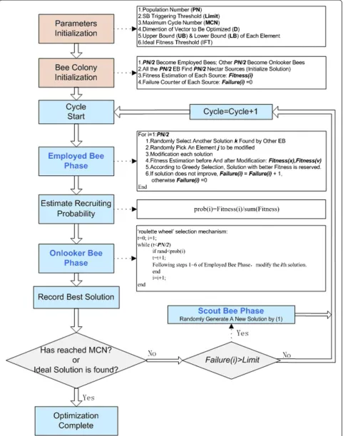
ABC algorithm is inspired by the foraging behavior of real bee colony. The objective of a bee colony is to maximize the nectar amount stored in the hive. The mission is implemented by all the members of the col-ony, by efficient division of labor and role transforming. Each bee performs one of following three kinds of roles: employed bees (EB), onlooker bees (OB), and scout bees (SB). They could transform from one role to another in different phases of foraging. The flow of nectar collec-tion is as follow:
1. In initial phase, there are only some SB and OB in the colony. SB are sent out to search for potential nectar source, and OB wait near the hive for being recruited. If any SB finds a nectar source, it will transform into EB.
2. EB collect some nectar and go back to the hive, and then dance with different forms to share information of the source with OB. Diverse forms of dance represent different quality of nectar source. 3. Each OB estimates quality of the nectar sources
found by all EB, then follows one of EB to the corresponding source. All OB choose EB according to some probability. Better sources (more nectar) are more attractive (with larger probability to be selected) to OB.
4. Once any sources are exhausted, the corresponding EB will abandon them, transform into SB and search for new source.
ordinary ones. Thus, the nectar collection is more effective.
Analogously, in ABC algorithm, position of nectar source is presented by the coordinate inD-dimensional space. It is the solution vector~x of some special prob-lem, and the quality of nectar source is presented by the objective function fð Þ~x of this problem. Accordingly, optimization of this problem is implemented by simulat-ing behaviors of the three kinds of bees. The flowchart of original ABC algorithm is shown in Figure 1. The main steps are as follow.
1. Parameters initialization of ABC algorithm. Population number (PN) and scout bee triggering
threshold (Limit) are the key parameters of ABC
algorithm. Maximum cycle number (MCN) or ideal fitness threshold (IFT) could be set for terminating algorithm. As stated in formula (1), all variables to
be optimized form aD-dimensional vector~x.
Restrict both upper bound (UB) and lower bound
(LB) of each variable.
2. Bee colony initialization. In ABC algorithm, since SB transform into EB, they are not reckoned in PN. Generally, the initial nectar sources are found by PN/2 SB, and then they all transform into EB. The other PN/2 bees are OB. The initial PN/2 solutions are generated by formula (2) in principle. Specified initial value could be used only if needed. All further modifications are based on these PN/2 solutions, which is corresponding to the PN/2 EB.
xð Þij ¼LBð Þj þϕð Þj
i UBð Þj LBð Þj
wherei¼1;2;. . .;PN=2 j¼1;2;. . .;D ð2Þ
wherexð Þij is thejth elements of theith solution.ϕð Þij is uniformly distributed random real number in the range of [0, 1]. Objective functionfð Þ~x is introduced to estimate the fitness of each solution~x. For parameter optimization of SVM classifier,fð Þ~x could be minimum classification error or maximum classification accuracy. VectorFailureis a counter, length PN/2, and is set to zero for counting optimizing failure of each EB.
3. Each cycle includes following phases:
1) Employed bee: Each EB randomly modifies single elementxð Þij of sourceiby formula (3). Then fitness of the two solutions (before and after modification) is estimated. Greedy selection criterion is introduced to choose the one with better fitness, and the reserved one becomes new solution of this EB. If fitness of EB is not
improved after modification, corresponding
Failurecounters will increase by 1.
xð Þij ¼xð Þij þλið Þj xð Þij xð Þkj
ð3Þ
wherexð Þij is defined as in formula (2), andxð Þij is the corresponding new element of the solution after modification.λð Þij is uniformly distributed
random real number in the range of [−1, 1], and
xð Þkj is thejth elements of~xk. Note thatk6¼i.
2)Estimate recruiting probability. By formula (4), fitness and recruiting probability of each EB are calculated.
FitnessðiÞ ¼ 1
1þfð Þ~xi
probðiÞ ¼ FitnessðiÞ
X
PN=2
i¼1
FitnessðiÞ
8 > > > > > > < > > > > > > :
ð4Þ
3)Onlooker bee:‘roulette wheel’selection mechanism is introduced. It forces each OB following one of EB according recruiting probability. Owing to better solutions
corresponding to larger recruiting probability, they obtain more chance to be optimized. Then each solution will be modified again by its followers (OB), using same steps as employed bee phase, from steps 1 to 6.
4)Record best solution. All PN/2 solutions after modification are ranked according to their fitness, and best solution of current cycle is reserved. The termination conditions are then checked. When cycle counter reach the MCN or an ideal solution is found (reach IFT), the algorithm is over. 5)Scout bee. IfFailurecounters of any solutions
exceedLimit, the corresponding solution is
abandoned, and scout bee is triggered. For
example, if thelth solution is abandoned, a new
solution is generated to replace the original one using formula (2), where seti = l.
By above operations, ABC algorithm performs
optimization. Nevertheless, in both EB and OB phases, the algorithm merely modify single element of the solution in each cycle. If the length of the solution vectorDis large, it makes inefficiency improvement in each cycle. In [2], MR is proposed, which is a real number factor in [0, 1]. For element xð Þij of solutioni, a uniformly distributed random real number (0≤Rð Þij≤1) is produced. If Rð Þij≤MR, element
are larger than MR, ensure at least one parameter being modified by original algorithm. Although this MR-ABC al-gorithm improves the convergence rate of basic alal-gorithm to some extent, its robustness is not ideal according to testing by abundant experiments.
D-ABC algorithm
The original idea of ABC algorithm is to perform hier-archical optimization. Overall, global searching is per-formed by EB and local searching is implemented by OB. However, this idea is not prominent in traditional ABC algorithms, because the modifying extent of EB and OB is similar and relatively fixed. Dynamic modify-ing extent is more reasonable. To achieve more effective optimization, the activity of bees must be dynamic in different stages of the algorithm. Our idea is that global searching should be dominant in early cycles and local searching should be primary in the posterior cycles. This could be more consistent with actions of real bees: EB become main force in the initial, then more and more OB follow, they play the major role afterwards. Specific-ally, in early stages of optimization, audaciously modify more elements of ~x in EB phase. That makes the bees approaching better solution by a greater probability. Fur-thermore, OB become active in posterior stages, and they modify more elements of~x. That provides more op-portunities to jump out of local optimal solution.
Consequently, we propose a dynamic‘activity’factor, and introduce it into modification operation of EB and OB phases. Adjust number of elements of the solution vector in each cycle. The‘activity’factorδcould be defined as follow-ing two forms by formulas (5) and (6), alternatively:
δ¼ΦðCc;MCN;DÞ ð5Þ
δ¼ΔðFc;IFT;DÞ ð6Þ
whereCcis current cycle number, ,Dis length of solution,
Fcis current best fitness. The alternation of the two
defini-tions depends on the termination condition of the algo-rithm. If using MCN to terminate the optimization, δ is defined as formula (5). And if IFT is employed,δis defined as formula (6).δEB andδOB are‘activity’factor of EB and
OB, respectively. Employ τ as the progress rate of the optimization,δEB andδOBsubject to: (1)δEBgrows withτ,
whenτis not beyond half of total progress.δEB2½0;1; (2)
δOBgrows withτ, when τis beyond half of total progress.
δOB2½0;1 . Explicit formulas could be determined
according to specific problems. In this article, following scheme is suggested when utilize MCN as termination con-dition of the algorithm.
(1)In early stages, for EB phase,δEBis defined as
formula (7). It reduces withCcincreasing, andNEB
elements are randomly picked to be modified; For OB phase, MR method is recommended. Audacious global modification and conservative local
modification are implemented.
Figure 2Flowchart of D-ABC algorithm-based multi-parameters optimization.It presents flowchart of optimizing process.
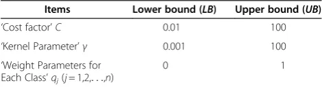
Table 1 Range of parameters to be optimized
Items Lower bound (LB) Upper bound (UB)
‘Cost factor’C 0.01 100
‘Kernel Parameter’γ 0.001 100 ‘Weight Parameters for
Each Class’qj(j= 1,2,. . .,n)
0 1
Table 2 Dataset declaration
Dataset Number of
samples
Number of features
Number of labels D
1. Wine classification 178 13 3 5
2.Image segment 2310 19 7 9
3.Building classification (a) 600 8 30 32 4.Building classification (b) 1000 8 50 52
Table 3 Parameters settings of different optimization algorithm
Algorithm IFT PN MR MCN Limit Run times ‘k-fold’ cross-validation
PSO 100 % 10 — 100 — 20 10
EB!NEB¼½δEBD ¼ 1 Cc
MCN
D
OB!MR
)
if Cc≤ MCN
2 ð7Þ
(2)In posterior stages, for EB phase, MR method is
reused; For OB phase,δOBis defined as formula (8).
It increases withCcgrowing, andNOBelements are
randomly picked to be modified. Conservative global modification and audacious local modification are implemented.
EB!MR
OB!NOB¼½δOBD¼ Cc MCND
)
if Cc> MCN
2
ð8Þ
Furthermore, D-ABC algorithm is closely to the length Dof solution vector. When Dis small, there is practic-ally little difference between original ABC algorithm and
D-ABC algorithm. And for larger D, the advantages of
D-ABC algorithm are prominent on convergence rate and improving the quality of solutions.
Multi-parameters optimization of SVM-based soft-margin classifier
Introduction of SVM parameters optimization
As we all know, training soft-margin classifier is a con-strained optimization problem as formula (9).l is num-ber of samples, xi is ith sample, and yi is the label of
samplei.
minimize 1
2‖w‖
2þCX l
i¼1
ζi
subject to yi½wxiþb≥1ζiðζi ≥0;i¼1;2;. . .;lÞ
ð9Þ
It is a quadratic programming problem, which max-imum the margin (2=‖w‖) when restricting the least clas-sification error rate.
To solve unbalanced problem of training samples, ‘slack variable’ (ζ) and ‘cost’ factor (C) are introduced to process outlier samples and compromise the pos-ition of optimal separating hyper-plane. Large C indi-cates attaching importance to the loss of outliers of different classes. SVM needs to assign different C for each class. If these cost factors are not properly set, poor classification result will be obtained. However, experience-based setting is not robust. As a result, the
Table 4 Initial objection value of different datasets
Initial accuracy EB1 (%) EB2 (%) EB3 (%) EB4 (%) EB5 (%) EB6 (%) EB7 (%) EB8 (%) EB9 (%) EB10 (%)
Dataset 1 40.44 40.45 40.44 40.45 40.44 40.44 40.44 40.44 40.44 56.18 Dataset 2 30.95 24.76 21.90 23.81 28.57 24.28 30.95 21.90 21.90 22.86
Dataset 3 72.5 72.5 72 71.5 71 71.67 71.17 70.83 71.17 71.83
Dataset 4 65.1 60.7 65.7 66.4 66.7 65.7 66.1 66.5 64.3 67.6
multi-parameters optimizing problem needs to be solved, and parameters to be optimized will increase with number of class.
Additionally, parameters of kernel function of SVM need to be optimized. Solving (9) with Lagrange multi-plier method, the separating classification function could
be obtained as formulas (10) and (11), where αi is
Lagrange factor.
w¼X
l
i¼1
αiyixi
ð Þ ð10Þ
g xð Þ ¼X
l
i¼1
aiy<xi;x>þb ð11Þ
When samples are linearly inseparable, SVM processes nonlinear problem as linear classification in high-dimensional, which is performed by kernel function as formula (12). Both number and type of parameters to be optimized are determined by the kernel function.
g xð Þ ¼X
l
i¼1
aiyK xð i;x;γÞ þb ð12Þ
All above parameters to be optimized compose a vec-tor~x, and the multi-parameters optimization problem is
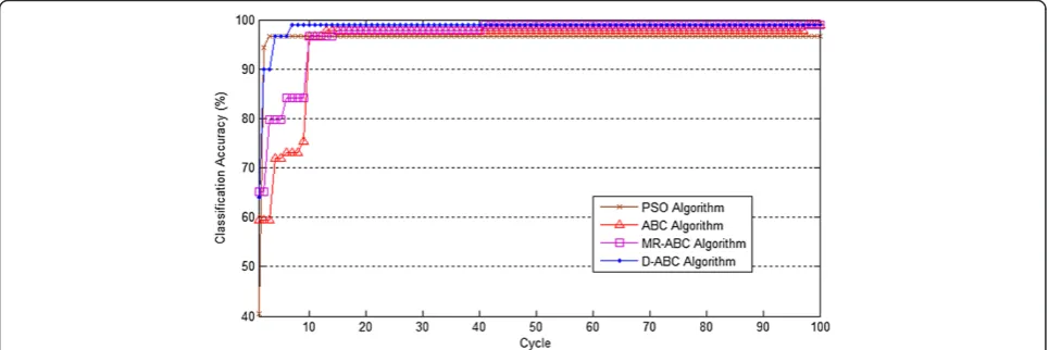
Figure 4Performance comparison of different algorithms for Dataset 2.X-axis presents number of cycles, andY-axis indicates classification accuracy after optimized by different algorithms.
defined as (13):
maximize fð Þ ¼~x f C;γ;q1;q2;. . .;qn
subject to yi½wxiþb≥1ζiðζi≥0;i¼1;2;. . .;lÞ
ð13Þ
whereCis the cost factor,γis the kernel parameter, and nis number of labelsqjðj¼1;2;. . .;nÞ, are weight
para-meters of each class, which set the cost factorCof class jtoq,C. Moreover, to obtain creditable classification ac-curacy,‘k-fold’cross-validation is utilized for testing per-formance of SVM classifier. In our experiments,kis set
to 10. Define the objective function fð Þ~x as the average classification accuracy of ‘10-fold’cross-validation as for-mula (14):
fð Þ ¼~x Xk
m¼1
Accuracym=k ð14Þ
Consequently, this problem could be solved by optimization algorithm. Owing to multiple parameters need to be optimized, our D-ABC algorithm is more suit-able than traditional ABC algorithm. The flowchart of D-ABC
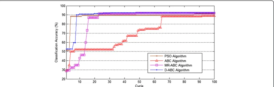
Figure 6Performance comparison of different algorithms for Dataset 4.X-axis presents number of cycles, andY-axis indicates classification accuracy after optimized by different algorithms.
algorithm based multi-parameters optimization is shown in Figure 2.
For a set of training samples, D-ABC algorithm modifies parameters vector ~x¼C;γ;q1;q2;. . .;qn
cycle-by-cycle, and search best ~x for maximizing the classification accuracy.
Experiments
In this article, multi-class SVM-based soft-margin classi-fier is performed by C-support vector classification (C-SVC) toolbox. It is from LIBSVM toolbox supplied by Cheng and Lin [14]. The toolbox supply several typical kernel functions. Radial basis function is employed as kernel function in our experiments, and kernel param-eterγneed to be optimized. Forn-class classification, all parameters to be optimized and their range are pre-sented in Table 1. Obviously, the length of vector ~x is D = n +2. The dataset utilized for SVM training is as Table 2 shows. ‘Wine’and‘Image Segment’are two typ-ical testing dataset, which are widely used for testing SVM-based classifier. The two‘building’datasets are collected by us especially for multi-parameters optimization problem.
Performances of PSO algorithm, original ABC algo-rithm, MR-ABC algoalgo-rithm, and D-ABC algorithm are compared for this optimization problem. All algorithms are coded under MATLAB 2011b. Main hardware
con-figuration of our computer: IntelWCore(TM)2 Duo CPU
[email protected] GHz 2.27 GHz, 2.00 GB RAM.
According to principle of fair comparison: (1) corre-sponding initialization parameters are same set in these
algorithms as Table 3 shows,the settings are according to [2]; (2) using same starting searching points to initialize the colony, as shown in Table 4 and Appendix. Mean value of 20 times running by different algorithms are collected as the final results for the four datasets, which are shown in Figures 3, 4, 5, and 6 and Table 4. Particu-larly, to verify the robustness of different algorithm, stand-ard deviations of the 20 times run are given by Figures 7 and 8, for the two high-dimensional datasets.
Note that we choose measuring the convergence rate in cycle for following reasons: Generally, computational time of calling objection function is much larger than other parts of ABC algorithm, particularly when our ob-jection function includes multiple times SVM training. The SVM training takes more than much time, and in each cycle, the code of objection function will be called many times (same times in each cycle for different algo-rithm, and times is determined by parameter PN). Ob-jection function calling occupies more than 90% computational time of both original ABC algorithm and modified ones (for instance, for dataset 4, about 22.3 s
"
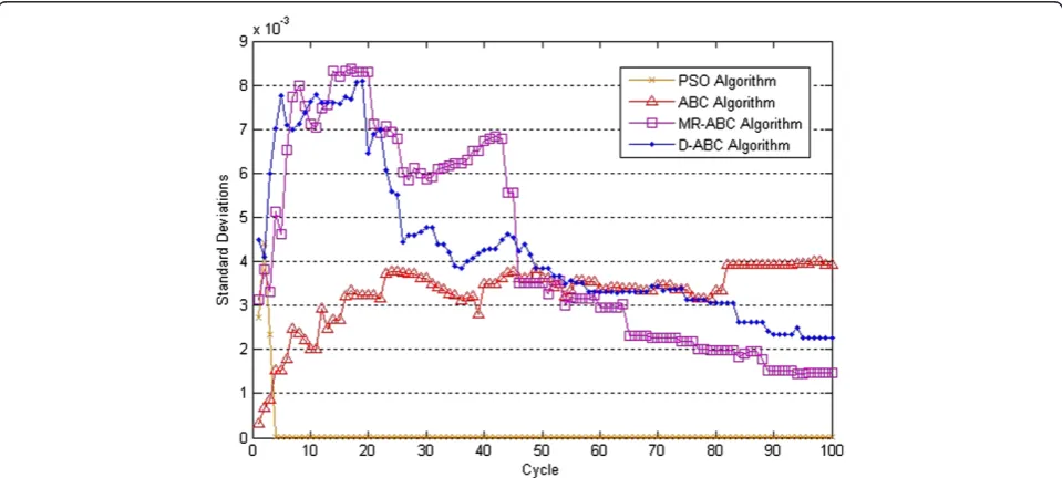
Figure 8Standard deviations of different algorithms for Dataset 4.X-axis presents number of cycles, andY-axis indicates standard deviations of classification accuracy after optimized by different algorithms for 20 times runs.
Table 5 Best solution obtained by different optimization algorithms
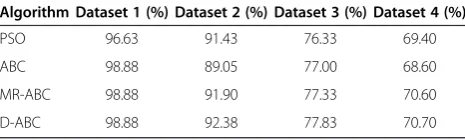
Algorithm Dataset 1 (%) Dataset 2 (%) Dataset 3 (%) Dataset 4 (%)
PSO 96.63 91.43 76.33 69.40
ABC 98.88 89.05 77.00 68.60
are cost by running D-ABC algorithm for each cycle, 21.7 s for MR-ABC algorithm, and 20.5 s for original ABC algorithm. It is obviously that objection function cost most time in each cycle). Moreover, every time the objection function is called, the solution is modified. Therefore, it is more reasonable measuring the convergence rate in cycle than in time. On the contrary, if measuring the conver-gence rate in specified computational time, each solution might be modified different times, which could be unfair.
As is shown in Figure 3, for dataset 1, D-ABC algorithm rapidly find a solution~x, with which SVM could best training the data and obtain a classification accuracy of 98.88 %, while original ABC algorithm and MR-ABC obtain that solution slowly. Though PSO algorithm has a good convergence rate, it could not get an ideal solution. As is shown in Figure 4, for dataset 2, similarly, compared with original ABC algorithm and MR-ABC, D-ABC algorithm performs better conver-gence rate and obtains higher classification accuracy, and the improvement is more obvious than dataset 1. PSO algorithm still converges fast but an unsatisfactory solution. By contrast, D-ABC algorithm obtains a classification accuracy of 92.38 %. The results above have demonstrated the advantages of D-ABC algorithm for lower dimension of parameter-vector like datasets 1 and 2. Furthermore, datasets 3 and 4 are col-lected for testing optimization of higher dimensional~x. As is shown in Figures 5, 6, and Table 5, similar conclusions could be obtained that D-ABC algorithm has certain advan-tages over other algorithms, which lead to greater improve-ment on convergence rate and quality of solution, especially whenDis larger. Moreover, standard deviations (of 20 times run) for the two groups of datasets are shown in Figures 7
and 8, respectively. The curves illustrate the standard devia-tions of objection function in different optimizing cycles, and the relatively lower standard deviations have been obtained by D-ABC algorithm for both datasets 3 and 4, which indicates that D-ABC algorithm has good robustness.
Conclusion and discussion
In this article, two parts of work have been studied. First, D-ABC algorithm is introduced to improve the disadvan-tages of traditional ABC algorithms: poor convergence rate and local optimizing. Second, D-ABC algorithm is utilized for multi-parameters optimization of SVM classifier. Experi-ments results demonstrate that D-ABC algorithm is in many ways superior to traditional ABC algorithms. It effect-ively ameliorates the convergence rate and local optimum. Typically, for multi-parameters optimization, when lengthD of vector (to be optimized) is larger, our study has provided substantial evidence for the advantages of D-ABC algorithm on quality of solution and convergence rate. When D-ABC algorithm is employed for optimizing multi-parameters of SVM-based soft-margin classifier, great improvement is obtained on performance of the classifier. Moreover, the ro-bustness of D-ABC algorithm is proofed. Furthermore, the idea of D-ABC algorithm could be associated with other modified ABC algorithms, whose modification is on other phase of original ABC algorithm, and it might further im-prove traditional ABC algorithm in future work.
Appendix
The starting searching points of the four group of experi-ments are tabulated in Tables 6, 7, 8, and 9.
Table 7 The initial colony of dataset 2
EB1 EB2 EB3 EB4 EB5 EB6 EB7 EB8 EB9 EB10
82.97033 84.92364 37.31617 59.35914 87.268 93.35681 66.87958 20.75697 65.41967 7.29795 406.7328 666.9349 933.7263 810.9519 484.5534 756.7516 417.0533 971.7863 987.9748 864.1489
0.388884 0.454742 0.246687 0.784423 0.882838 0.913712 0.558285 0.598868 0.148877 0.899713 0.450394 0.205672 0.899651 0.762586 0.882486 0.28495 0.673226 0.66428 0.122815 0.407318 0.275287 0.71667 0.283384 0.896199 0.826579 0.390027 0.497903 0.694805 0.834369 0.60963 0.574737 0.326042 0.456425 0.713796 0.884405 0.720856 0.018613 0.674776 0.438509 0.43782 0.117037 0.814682 0.324855 0.246228 0.342713 0.375692 0.546554 0.56192 0.395822 0.398131 0.515367 0.657531 0.950915 0.722349 0.40008 0.831871 0.134338 0.060467 0.084247 0.163898 0.32422 0.301727 0.011681 0.539905 0.095373 0.146515 0.631141 0.85932 0.974222 0.570838 Table 6 The initial colony of dataset 1
EB1 EB2 EB3 EB4 EB5 EB6 EB7 EB8 EB9 EB10
Table 8 The initial colony of dataset 3
EB1 EB2 EB3 EB4 EB5 EB6 EB7 EB8 EB9 EB10
81.4909 90.58861 12.78598 91.34625 63.27269 9.844286 27.92197 54.73346 95.75493 96.49236 157.6215 970.5931 957.1674 485.3808 800.2825 141.8949 421.7671 915.7364 792.2094 959.4928
0.655741 0.035712 0.849129 0.933993 0.678735 0.75774 0.743132 0.392227 0.655478 0.171187 0.706046 0.031833 0.276923 0.046171 0.097132 0.823458 0.694829 0.317099 0.950222 0.034446 0.438744 0.381558 0.765517 0.7952 0.186873 0.489764 0.445586 0.646313 0.709365 0.754687 0.276025 0.679703 0.655098 0.162612 0.118998 0.498364 0.959744 0.340386 0.585268 0.223812 0.751267 0.255095 0.505957 0.699077 0.890903 0.959291 0.547216 0.138624 0.149294 0.257508 0.840717 0.254282 0.814285 0.243525 0.929264 0.349984 0.196595 0.251084 0.616045 0.473289 0.35166 0.830829 0.585264 0.549724 0.917194 0.285839 0.7572 0.753729 0.380446 0.567822 0.075854 0.05395 0.530798 0.779167 0.934011 0.129906 0.568824 0.469391 0.011902 0.337123 0.162182 0.794285 0.311215 0.528533 0.165649 0.601982 0.262971 0.654079 0.689215 0.748152 0.450542 0.083821 0.228977 0.913337 0.152378 0.825817 0.538342 0.996135 0.078176 0.442678 0.106653 0.961898 0.004634 0.77491 0.817303 0.868695 0.084436 0.399783 0.25987 0.800068 0.431414 0.910648 0.181847 0.263803 0.145539 0.136069 0.869292 0.579705 0.54986 0.144955 0.853031 0.622055 0.350952 0.51325 0.401808 0.075967 0.239916 0.123319 0.183908 0.239953 0.417267 0.049654 0.902716 0.944787 0.490864 0.489253 0.337719 0.900054 0.369247 0.111203 0.780252 0.389739 0.241691 0.403912 0.096455 0.131973 0.942051 0.956135 0.575209 0.05978 0.23478 0.353159 0.821194 0.015403 0.043024 0.16899 0.649115 0.731722 0.647746 0.450924 0.547009 0.296321 0.744693 0.188955 0.686775 0.183511 0.368485 0.625619 0.780227 0.081126 0.929386 0.775713 0.486792 0.435859 0.446784 0.306349 0.508509 0.510772 0.817628 0.794831 0.644318 0.378609 0.81158 0.532826 0.350727 0.939002 0.875943 0.550156 0.622475 0.587045 0.207742 0.301246 0.470923 0.230488 0.844309 0.194764 0.225922 0.170708 0.227664 0.435699 0.311102 0.92338 0.430207 0.184816 0.904881 0.979748 0.43887 0.111119 0.258065 0.40872 0.594896 0.262212 0.602843 0.711216 0.221747 0.117418 0.296676 0.318778 0.424167 0.507858 0.085516 0.262482 0.801015 0.02922 0.928854 0.730331 0.488609 0.578525 0.237284 0.458849 0.963089 0.546806 0.521136 0.231594 0.488898 0.62406 0.679136 0.395515 0.367437 0.987982 0.037739 0.885168 0.913287 0.796184 0.098712 0.261871 0.335357 0.679728 0.136553 0.721227 0.106762 0.653757 0.494174 0.779052 0.715037 0.903721 0.890923 0.334163 0.698746 0.19781 0.030541 0.744074 0.500022 0.479922 0.904722 0.609867 0.617666 0.859442 0.805489 0.576722 0.182922 0.239932 0.886512 0.028674 0.489901 0.167927 0.978681 0.712694 0.500472 0.471088 0.059619 0.681972 0.042431 0.071445 0.52165 0.09673 0.818149 0.817547 0.72244 0.149865 0.659605 0.518595 0.972975 0.648991 0.800331 0.453798 0.432392 0.825314 0.08347 0.133171
Table 9 The initial colony of dataset 4
EB1 EB2 EB3 EB4 EB5 EB6 EB7 EB8 EB9 EB10
17.42152 39.15469 83.15484 80.3561 6.141071 39.98585 52.7349 41.73827 65.7203 62.83454 291.9912 431.6569 15.49697 984.0639 167.1767 106.2253 372.416 198.1264 489.6927 339.5
Table 9 The initial colony of dataset 4(Continued)
Abbreviations
ABC: Artificial bee colony; D-ABC: Dynamic artificial bee colony; EB: Employed bees; PSO: Particle swarm optimization; RSEM: Randomly single element modification; IFT: Ideal fitness threshold; LB: Lower bound; MCN: Maximum cycle number; MR: Modification rate; MR-ABC: Modification rate artificial bee colony; OB: Onlooker bees; PN: Population number; SB: Scout bees; SVM: Support vector machine; UB: Upper bound.
Competing interests
The authors declare that they have no competing interests.
Author details
1Department of information engineering, Harbin institute of technology, (92 West Dazhi Street ), Harbin (150001), China.2Department of information engineering, Harbin institute of technology, (92 West Dazhi Street ), Harbin (150001), China.3Department of modern control, Institute of automation of Heilongjiang academy of Science, (Hanshui road), Harbin (150090), China.
Received: 6 March 2012 Accepted: 6 July 2012 Published: 24 July 2012
References
1. D. Karaboga,An Idea Based on Honey Bee Swarm for Numerical Optimization. Technical Report, TR06(Erciyes University Press, Erciyes, 2005)
2. D. Karaboga, B. Akay, A modified artificial bee colony (ABC) algorithm for constrained optimization problems. Appl. Soft Comput.11(3), 3021–3031 (2010). doi:10.1016/j.asoc.2010.12.001
3. B. Akay, D. Karaboga, A modified artificial bee colony algorithm for real-parameter optimization. Inf. Sci192, 120–142 (2012). doi:10.1016/j. ins.2010.07.015
4. A. Singh, An artificial bee colony algorithm for the leaf-constrained minimum spanning tree problem. Appl. Soft Comput.9(2), 625–631 (2010). doi:10.1016/j.asoc.2008.09.001
5. L. Bao, J. Zeng,Comparison and analysis of the selection mechanism in the artificial bee colony algorithm, 1st edn. (Paper presented at Ninth International Conference on Hybrid Intelligent Systems (HIS '09), Shenyang, LiaoNing, China, 2009), pp. 411–416
6. R.S. Parpinelli, C.M.V. Benitez, H.S. Lopes, Parallel approaches for the artificial bee colony algorithm, handbook of swarm intelligence: concepts. Princ. Appl.8, 329 (2011)
7. D. Haijun, F. Qingxian, Artificial bee colony algorithm based on Boltzmann selection policy. Comput. Eng. Appl.45(31), 53–55 (2009)
8. P. Tsai, J. Pan, B. Liao, S. Chu,Interactive artificial bee colony (IABC) optimization(ISI2008, Taipei Taiwan, 2008)
9. R. Akbari, A. Mohammadi, K. Ziarati, A novel bee swarm optimization algorithm for numerical function optimization. Commun. Nonlinear Sci. Numer. Simul15, 3142–3155 (2010). doi:10.1016/j.cnsns.2009.11.003 10. C. Cortes, V. Vapnik, Support-vector networks. Mach. Learn20, 273–297
(1995). doi:10.1007/BF00994018
11. F. Samadzadegan, A. Soleymani, R.A. Abbaspour,Evaluation of Genetic Algorithms for tuning SVM parameters in multi-class problems(Paper presented at 11th International Symposium on Computational Intelligence and Informatics (CINTI), Budapest, 2010), pp. 323–328
12. L. Yang, H.T. Wang,Classification based on particle swarm optimization for least square support vector machines training(Paper presented at Third International Symposium on Intelligent Information Technology and Security Informatics (IITSI), Jinggangshan, 2010), pp. 246–249 13. T.J. Hsieh, W.C. Yeh, Knowledge discovery employing grid scheme least
squares support vector machines based on orthogonal design bee colony algorithm. IEEE Trans. Syst. Man Cybern. B: Cybernetics41(5), 1–15 (2011). doi:10.1109/TSMCB.2011.2116007
14. C.C. Chang, C.J. Lin, LIBSVM: a library for support vector machines. ACM Trans. Intell. Syst. Technol. (TIST)2(3), 27 (2011). doi:10.1145/ 1961189.1961199
doi:10.1186/1687-6180-2012-160
Cite this article as:Yanet al.:Dynamic artificial bee colony algorithm for multi-parameters optimization of support vector machine-based soft-margin classifier.EURASIP Journal on Advances in Signal Processing2012
2012:146.
Submit your manuscript to a
journal and benefi t from:
7Convenient online submission
7Rigorous peer review
7Immediate publication on acceptance
7Open access: articles freely available online
7High visibility within the fi eld
7Retaining the copyright to your article