Equivalent differential equations for nonlinear dynamical systems

(1)

Thesis by Edward John Patula

In Partial Fulfi.llment of the Requirements For the Degree of

Doctor of Philosophy

California Institute of Technology Pasadena, California

1970

(2)

(ii)

ACKNOWLEDGEMENTS

The author wishes to express his sincere appreciation to Professor W . D. !wan, whose guidance and encourage1nent made this investigation possible. The assistance of the faculty in the Applied Mechanics Department, who have been so helpful in so many ways, is gratefully acknowledged.

The author wishes to thank Mrs. Odessa Walker, Miss JuH~ Wright, and Mrs. Phyllis Henderson for the very competent typing of the manuscript, and also Miss Cecilia Lin for h.~r assistance.

The author would also like to express his appreciation to the California Institute of Technology for the financial assistance

r:~ceived dm·-i..ng the cour;:.;e of this study.

(3)

ABSTRACT

A technique for obtaining approximate periodic solutions to nonlinear ordinary differential equations is investigated. The approach is based on defining an equivalent differential equation whose exact periodic solution is known. Emphasis is placed on the mathematical justification of the approach. The relationship

between the differential equation error and the solution error is investigated, and, under certain conditions, bounds are obtained on the latter. The technique employed is to consider the equation governing the exact solution error as a two point boundary value problem. Among other things, the analysis indicates that if an exact periodic solution to the original system exists, it is always possible to bound the error by selecting an appropriate equivalent

system.

Three equivalence criteria for minimizing the differential equation error are compared, namely, minimum mean square error, minimum mean absolute value error, and minimum maximum

absolute value error. The problem is analyzed by way of example, and it is concluded that, on the average, the minimum mean square error is the most appropriate criterion to use.

A comparison is made between the use of linear and cubic auxiliary systems for obtaining approximate solutions. In the examples considered, the cubic system provides noticeable

(4)

(iv)

(5)

COMPARISON OF VARIOUS EQUIVALENCE CRITERIA

Preliminaries

Description of the Minimization Procedures Example l

Example 2 Example 3 Example 4 Conclusions

A COMPARISON OF LINEAR AND CUBIC APPROXIMATIONS FOR SECOND ORDER SCALAR SYSTEMS

General Linear Approximation General Cubic Approximation

54

72

93

105 106 109 112 117 140 147

1

5

4

(6)

Part

5.3 5.4

Example 1 Example 2

(vi)

Title

CHAPTER VI. RELATION OF THE EQUIVALENT EQUATION APPROACH TO OTHER APPROXIMATE

167 171

TECHNIQUES 186

6. 1

6.2

Method of Weighted Residuals

Anomalies Associated with the Method of Least Squares and Other Averaging Techniques

CHAPTER VII. SUMMARY AND CONCLUSIONS LIST OF REFERENCES

186

(7)

I. INTRODUCTION

The area of nonlinear ordinary differential equations has been investigated by mathematicians for centuries. However, it has only been in recent times that the engineer and the applied theoretician have developed an interest in this area. One major reason for this interest is that it is not always possible to neglect nonlinearities in many of today's complex problems. In situations where a more detailed

under-standing of the qualitative and quantitative behavior of systems is desired, it is often necessary to include nonlinear effects. Although nonlinear equations have occupied the mathematician for quite some time, the techniques available for obtaining exact closed form solutions are rather limited. Under suitable conditions, existence and uniqueness

of solutions can be proved, but for only a relatively small number of nonlinear equations are the exact solutions known. A good treatment of the existence and uniqueness issue is given in reference (1 ).

The inability to obtain exact solutions has necessitated the development of approximate analysis for studying nonlinear problems. This analysis may loosely be divided into two categories: topological methods and approximate solution methods. The former usually involve phase plane or functional analysis methods. The Poincar~ theory(Z )for the singular points of two-dimensional autonomous systems and the S-econd Method of Liapunov (3)for the stability of nonlinear

(8)

-

2-methods, on the other hand, usually involve obtaining closed form approximate solutions for the nonlinear system of interest. Typical examples of this category are the Poincar~-Linstead perturbation technique(4)and the asymptotic methods of Krylov, Bogoliubov, and Mitropolsky ( 5).

(9)

The present investigation involves an approximate technique which may be classified as an approximate solution method. The approach, called the equivalent equation approach, was presented in

several recent papers by Iwan (6, ?)and is designed to provide approxi-mate periodic solutions to nonlinear systems. The technique is a

generalization of the method of equivalent linearization and is based on defining an alternative or auxiliary differential system whose exact periodic solution is known.

Most standard approximating techniques involve assuming a certain solution form containing unspecified parameters. These param-eters may be prescribed by minimizing, in some sense, the error

residual obtained by substituting the assumed solution into the original differential system. Since periodic motions are of interest, the usual

solution form involves linear combinations of trigonometric functions. Typical methods which fall into this class are: The Poincare'-Linstead perturbation technique (4), Krylov-Bogoliubov-Mitropolsky asymptotic methods (S), Galerkin's technique ( 9 ), and the methods of collocation,

bd . d l (l O) 0 . i· . .

su omain, an east squares . ne maJor imitation on most of the above techniques is that the usual first order approximation they provide is accurate only for equations which are nearly linear.

In-creased accuracy is possible by including more terms in the

(10)

-4-m.oderately large nonlinearities and which, at the same time, involve levels of computational effort corriparable to the standard first order techniques.

Various other authors have utilized non-trigonometric solution forn1s in order to achieve rr1ore accuracy. Eringen postulated a gener-alized Galerkin1_{s procedure utilizing non-trigonometric solutions(ll).} Klotter and Cobb used a polynomial approximation to represent the quarter period wave form(lZ), The parameters were determined utilizing Galerkin1 _{s procedure. Recently, Barkham and Soudack used} solution forms which i1111dve Jacobian elliptic functions(l3, 14). Their technique utilized the method of slowly varying parameters and enabled transient behavior to be analyzed. However, they make several sim-plifying assumptions which detract from the rigor of the approach. Furthermore, their results apply only to second order equations which are "Duffing- like". The equivalent equation approach is like the above in that it represents an attempt to provide an unambiguous technique for systematically treating equations containing moderately large nonlinearities.

The idea of using one differential system to model another differential system is not new. The method of equivalent linearization has been an accepted approximate technique for quite some time.

Various authors have suggested modifications but these mainly concern the manner in which the linear system is made equivalent to the original

(11)

polynomial approximation where the nonlinearity is expanded in a . f 1 h . 1 1 . 1 ( 1 5• 16 ) 0 1 h 1.

series o u trasp er1ca po ynom1a s . n y t e inear term is utilized, and, therefore, an equivalent linear system is generated.

An example of using a nonlinear auxiliary system was given by Helfenstein (I?). He utilized Duffing' s equation with Jacobian cosine excitation to model Duffing's equation with trigonometric cosine excitation. However, the equivalent system is obtained by merely equating the coefficients of all like terms. This idea of using one nonlinear system to model another nonlinear system was the moti-vating factor in the development of the equivalent equation approach. By using nonlinear auxiliary systems, it is felt that better approxi-mations could be obtained since some of the features peculiar to

non-linear problems would be incorporated into the analysis in a very natural manner.

A complete description of the equivalent equation approach is given in Chapter II. As stated earlier, the approach is based on de-fining equivalent differential equations whose exact periodic solutions are known. By developing an alternative differential equation which is, in some sense, equivalent to the original system of interest, it is hoped that the corresponding periodic solution will also be equivalent to the exact solution of the original system. To illustrate the t echni-que, Section 2. 2 presents an example where the equivalent equation approach is used to obtain an approximate periodic solution to the un-damped Duffing1_s _equation_{with trigonometric excitation. Th}_e_auxiliary system utilized is Duffing 1

(12)

In Chapter III, the relationship between the differ<~ntial equation error (the difference between the original system and the equivalent system) and the solution error (the difference between the exact periodic solution and the s elution of the equivalent system) is investigated. Under certain conditions, bounds are obtained on the solution error in terms of the differential equation error. The tech-nique employed is to consider the equation governing the exact solution error as a two point boundary value problem. Rewriting the problem as an integral equation and using the Green's function, the method of successive approximations is applied to obtain a bound on the exact error. Among other things, the above analysis indicates that if an exact periodic solution to the original system exists, it is always possible to bound the error by selecting an appropriate equivalent system. Other authors have obtained results similar to those

pre-. .(18 19) (20 21 22)

sented 1n Chapter III. Some are Cesari ' , Urabe ' ' ,

. (23 24) (2 5) (26)

McLaughlin ' , Holtzman , and Lazer . Unfortunately, most of the above consider either weakly nonlinear equations or

specific auxiliary systems. The present analysis attempts to be more general by considering two arbitrary differential systems. That

research which seems to be most closely related to the present

work is discussed in Section 3. l.

(13)

In Section 3. 2, the results arc specialized for the case of

second order scalar equations. Furthermore, the Green 1

s function used in Section .3. 1 is associated with the unique linear part of the

error differential equation. In general, this equation contains periodic coefficients which makes the determination of the Green's function

very tedious. To avoid this difficulty the problem is reformulated utilizing the Green1 _{s function for a system with}_c_{onstant coefficients}_.

These coefficients are then selected by minimizing the resulting error

bound.

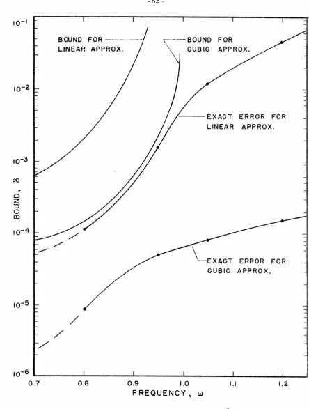
Section 3. 3 presents an example where the theory of Section 3. 2 is applied to the example considered in Section 2. 2, i.e. , the

trigo-nometrically excited undamped Duffing' s equation. Bounds are obtained for both the linear and cubic approximations.

An example of a conservative autonomous system is considered

in S~ction 3. 4. As mentioned above, the theory of Section 3. 2 yields

very little information concerning autonomous systems. Consequently, an alternative comparison technique is developed for second order

scalar conservative autonomous systems. The autonomous example considered is the undamped Duffing' s equation.

The manner in which an alternative system is made equivalent to the original system is examined in Chapter IV. Various equivalence

criteria are compared; namely, minimization of the mean square d if-ferential equation error, minimization of the mean absolute value differential equation error, and minimization of the maximum absolute

(14)

-8-respect to parameters appearing in the auxiliary system. The above errors were selected because of their physical relevance and their

relation to the error bound analysis performed in Chapter III. Since it was of interest to determine which equivalence cri-terion yielded the smallest actual solution error on the average, it was impossible to use analytical techniques to investigate the problem. Therefore, the problem is analyzed by way of example, and it is

concluded that, on the averag~ the minimum mean square error is the most appropriate equivalence criterion to use.

In Chapter V, a comparison is made between the linear and the cubic approximations for second order scalar systems. The general approximations are developed, and the determining equations are presented. The two approximations are compared by way of example. The specific examples considered are Duffing' s equation with trigonometric excitation, and a system of the form

~+ ~l

x =F cos (wt) .

l+a.JxJ ( 1 . 1 )

In both cases, the cubic approximation provides considerable improvement in solution accuracy over the linear system. In addition, in the second example there exists some indication that the cubic ap-proximation, which is, primarily, a harmonic approximation, is trying to yield some information about the ultraharmonic behavior

of ( 1 . 1).

(15)

techniques. The techniques considered are collocation, subdomain, least squares, and Galerkin' s procedure. The relation of these tech-niques to the general method of weighted residuals (2 7

l

is included.

(16)

l 0

-II. EQUIVALENT EQUATION APPROACH

In this chapter, the Equivalent Equation ~roach is presented. The description closely parallels that given by !wan ( 6 ) . An example of the use of the technique to obtain an approximate periodic solution for the undamped Duffing' s equation with trigonometric excitation is

incluclcd.

2 .1. Description of the Technique_

Consider the problem of obtaining an approximate solution for

the periodic motions of a system of ordinary differential equations.

The system of interest, called the original system, will be repre-sented as

D(~(t), t)

=

_Q (2. 1)

where D is a vector system which may contain differential operators

operating on the dependent vector x and functions of the independent variable t. F'urthcrmore, (2. I) is assumed to possess periodic solutions with least period T . For nonautonomm.1s systems, T may

s s

be prescribed by the excitation, but in the case of autono1nous systems, T may be an unknown of the problem.

s

In order to obtain an approximate solution of (2. I), consider

another system of equations, the auxilia!_Y ~tern, represented as

D-:<(~(t),a

1

,az,

...

,ar,t)=_Q (2.2)

(17)

known periodic solution forms that are members of some class of functions C having the form

~(t) = y([31' ... '[3s' t) (2. 3)

where (3.(j=l, ... , s) are parameters which define the members of C. If J

the solution of (2. 2) is unique, there will exist s relations between a. 1

and [3. which come directly from (2.2) plus any periodicity and/or J

initial conditions that may apply. Knowledge of the a. (i=l, ... , r) implies 1

a unique determination of the [3.(j=l, ... , s), but the converse is not J

necessarily true.

It is possible to obtain an approximate solution of (2. 1) by using the solution of an auxiliary system (2. 2) where the auxiliary

system is chosen to be as "close'' to the original system (2. 1) as I

possible. By close, it is meant that the equations comprising the original system and the auxiliary system are very similar in form. It is then hoped that, by making the difference in the governing

equations small, the difference in their respective solutions will also be small. In Chapter III, the nature of the relation between the dif-ference in the governing equations and the difference in their solutions is investigated, and the following statement is proved.

(18)

-12-Motivated by the above argument, one may select certain of

;~ the parameters a.(i=l, ... , r} so as to make some of the terms in D

1

identical in form to· terms in D. Let

*

D (x(t},

a

1, ... ,

a. ,

t}

=

D1 ~(t},

a

1, ... ,

a ,

t}

+

- - r - p

*

.!?

₂~(t}, ap+l •... , ar' t)

and

D~(t}, t}

=

p

1 ~(t}, t}

+p

2 ~(t}, t}

where

a. (i=l, ...

, p) are selected so that 1

' (2. 4}

(2. 5}

(2. 6)

The additional a.i (i=p+l, ... , r} parameters are determined in some manner so as to minimize the remaining difference between

D~

and D

for all members ~the class C; i.e. for all~(t} having the form x(t} = y(t}. where y(t) is notation for _-_y(

f31 ' ... '

13

_s

'

t).

Define the differential equation error 2(t) as the difference

~'<

obtained between D(x(t}, t} and D (x(t}, t} when both are evaluated at the

solution form y(t}. Then,

*

~(t} == f>(y(t), t} -

Q

(y(t}, t) (2. 7)

:;::;:

In (2. 7),

Q

(y(t}, t) does not vanish since the s relations betw-een the a..(i=l, ... , r) and the (3.(j=l, ... , s) have not been utilized. Using (2.4),

l J

(2. 5), and (2.6), equation (2. 7) can be written as ~'<

e:(a. +

1, ... ,a. ,t) = D2'"(t},t)- D2(y(t),a +1, ... ,a ,t).

- p r _u: - p r (2. 8)

where the explicit dependence of e: on the a.(i=p+l, ... , r) is indicated.

- 1

(19)

The et. (i=p+l, ... , r) are now selected so that (2. 8) is minimized.

l

However, there are many ways that (2. 8) could be minimized depending on the specific type of minimization desired. For example, the maxi-mum norm of g_ could be minimized, or the mean value of the norm of _£over one cycle of the motion could be minimized, or € could be made

to vanish at certain preselected points. In Chapter IV, approximations obtained by using these various minimization conditions are compared. As expected, no one minimization condition gives the "be st" approxi-mation in all cases. However, it may be concluded, in a very broad sense, that the optimum minimization criterion is

1

T

s

tl+Ts .

J

_?'

~dt

= minimum tl

(2. 9)

where T denotes the transpose, and t₁is an arbitrary time. Since the minimization of the integral is with respect to et.(i=p+l, ... , r), (2. 9) is

1

equivalent to

[

t +T

J

o

I 1 s T

__ I

€ e:dt =

o

oa.

T -

-1 s t

. 1

i=p+l, ... , r .

Since T does not depend on a.(i=p+l, ... , r) (remembering that the

s 1

j3.(j=l, •.. , s) are still arbitrary), (2. 10) becomes J

l l + T s [

~~ ~+_fT~~-J

dt=O, i=p+l, ... , r

1 l

t1

(2. 1 O)

(2 . 11 )

Because the s relations between the Ct.(i=l, ... , r) and the f3.(j=l, ... , s)

l J

(20)

-14-which <h~tennine the auxiliary 1:1ystcm paran1eter1:1 a .. (i I, ... ,r) which ar .. · 1

valid for all members of C. If these s relations are now introdui:.~d.

equation (2 .11) can be further reduced. Since the differentiation in

equation (2 .11) is with respect to explicit a.(i=p+l, ... ,r), the derivatives

i

T

*

of

£

may be expressed, using equation (2. 8), in terms of D

2 (y(t),

a

1, ...

,a ,

t) only·. Furthermore, E: tnay be expressed in ter1ns of

p+ r

-*

D(y(t)) only from equation (2 .7). D (y(t),t) vanishes once the s relations

are utilized. From the above considerations, equation (2 .11) becomes

J

tl+Ts 8 ~ [ _!?₂

,:;I'

(y(t), ap+l" .. , ar' t)

J

D(y(t), t)dt

=

0 ,

.

i=p+l_, ... , r. (2. 12)

t 1

1

It is as surned that the relations in (2 .12) will be of such a form

that it is possible to determine the a'lL"<iliary system parameters

a.(i=p+l, ... , r) and j3.(j=l, ... ,s) so that meaningful approximate solutions

1 J

and equivalent system equations are obtained. The values of the

para-meters generated by (2 . .12) correspond 1o extremums of the mean square

error (2. 9). These extremums may be either maximums or minimums.

Care must be taken to select only those values of

er

.•

(i=p+l, ... , r} and 1

13.(j=l, ... , s) which minimize (2. 9). If the weight functions J

ar':;r

..,

W.(t) ::: ~I D₂ (y(t),

a

+I' ... ,

a.

)j,

i=p+l, ... , r ,

1 ai - p r (2. 13)

are independent of a..(i=p+l, ... , r}, it can be shown that all solutions

1

generated by (2 .12) correspond to minimums of (2 .9). This situation

occurs if € is linear in the a.(i=p+l, ... ,r), which is often the case.

- 1

However, if the W.(t) depend on some of the a.(i=p+l, ... , r), various

1 1

(21)

be generated, even though an exact solution exists, or 2) some

extraneous approximate solutions could be introduced, or 3) a com

bi-nation of 1) and 2) above could occur. This particular point is

investi-gated in more detail in Chapter VI, where the equivalent equation

approach and the method of leasr squares are comparld. It suffices

a

,.J'

at this point to assume that -<:1- D

2''' (_y(t),

a

1, ... , Cl ,t) (i=p+l, ... , r) are

U(l. - p+ r

1

of a form that provide meaningful approximate solutio::is.

Let q be the number of independent equations gene rated by the

minimization condition (2 .12). Then, if q =r-p, the equations from

(2 .12) plus the s relations from the au_~iliary system (2 .2) combined

with the p preselected parameters a.(i=l, ... , p) satisfying (2. 6) will 1

determine all of the parameters a.(i=p+l, ... , r) and P.(j=l, ... , s). One

1 J

obtains not only a:i:i approximate solution) but also an "equivalent"

auxiliary system. This additional information m~y be quite useful.

For example, it rriight be of interest to know the equivalent mass or

the equivalent excitation level or the equivalent stiffness of s01ne

ori-ginal system, and the equivalent system approach would provide an

auxiliary system whose behavior, presu1nably would be better unde

r-stood. If q

<

r-p, it means that there are not enough independent

relations to determine all of the parameters, and that an additional

r-p-q relations have to be supplied. There are several ways in which

these additional relations may be obtained. One approach might be to

simply prescribe an additional r-p-q parameters in the auxiliary

system. However, depending on the specific parameters being

pre-scribed, fewer relations might be obtained from the minimization con

(22)

-16-would have to be specified until enough independent equations were obtained to determine all of the a..(i=l, ... , r) and 13.(j=l, .. ., s). An

l J

alternative approach to prescribing additional auxiliary system parameters is to generate an additional r-p-q equations from the q equations resulting from (2. 12). Consider an alternative form of equations (2 .12),

*

~

-Q

₂(y(t), a.p+l' ... , ar)}dt = 0 , i=p+l, ... , ' (2 . 14)

which is obtained by using equations (2.4), (2. 5), (2.6) and the s relations for the auxiliary system. In general, any differential system

Q

contains terms which can be put into the following

categories: l) terms containing only the highest order derivative of the vector function~·(_!?~; 2) terms containing only lower order deri-vatives of ~.(_D)B; and 3) terms which depend only on the independent

~' variable t, (D)C. If

Q

2 and

Q

2 are both separated into the above terms, equations (2. 14) become

where the functional

+<!?z)c-(!?;)c]dt=O , i=p+l, ... , r, (2.15)

dependence of D

(23)

entire combination. Utilizing this approach, (2 .15) may be decomposed to give

(2. 16)

'

where i can take on as many values in the set p+l, ... , r as are needed to

generate enough equations so that all of the auxiliary system pa rame-ters a.(i=l, ... ,r) andf3.(j=l, ... ,s) can be determined. Depending on

l J

::c

the specific D and~ chosen, certain of the equations in (2. 14) will lend themselves more naturally to the type of separation given in(2.16). Equations (2.16) have a physical interpretation as well. By separating

terms, one is attempting to represent certain types of tenns in the

original system by the same type of terms in the auxiliary system;

-

·

that is, one is asking that the highest derivative terms in~; model

the highest derivative terms in ~z· and that the terms depe!lding only

>!'

on t in D

2 model the terms depending only on t in ~

2

, etc. If the separated equations (2 .16} still do not provide sufficient equationa to

determine the auxiliary system parameters, it is possible to further divide the ter1ns in D into inorc categories. In t:hi:3 way, it is always

possible to generate a sufficient nu1nber of equationd to d1•h·rinine <.1. I l of the

a

.

and

13

.

(24)

-18-The problem of determining the solution parameters f).(j :: l, ... , s)

J

>!<

is simplified considerably if

Q

₂is a linear function of a.i (i=p+l, ... , r) and q=s. In this case, (3.(j=l, ... , s) may be determined directly from

J

equations (2. 12) without using the differential equations (2. 2) or fir st determining the parameters

a.

.

(i=p+l, ... , r). This would certainly be

l

*

the case when!? is a set of linear differential equations with constant coefficients o..(i=l, ... , r) and the class C contains the least number of

l

functions necessary to describe the periodic solution. The above formulation then becomes a generalization of the method of equivalent 1inear1zation . . . ( 8 ) . However, t e equivalent equation approach is not h . restricted to using only linear auxiliary systems. Indeed, one of the more important aspects of the equivalent equation approach is that it allows for the possibility of using one nonlinear system to model another nonlinear system.

The similarity in the form of equations (2. 12) to those obtained by application of Galerkin's method is apparent ( 9 ). In fact, the two approaches can give identical approximations depending on the set of trial functions used in Galerk.in's method. This point is considered in more detail in Chapter VI, where the two techniques are compared. In general, however, the results of the equivalent equation approach will differ from those of Galerkin's method.

As noted earlier, the present approach is essentially that of defining an equivalent system for the set D. As such, the j3.(j=l, ... , s)

J

remain arbitrary in equation (2. 8), and £has the significance of a difference term. The functional relationship between a..(i=l, ... , r) and

(25)

13.(j=l, ... , s) is not introduced until (2 .12). However, it is clear from

J

(2. 8) that ~ could also have been thought of as the error residual of the set of equations D'"(t), _{_u.} t) if the relations between a.(i_l =l, ... , r) and 13.(j=l, ... , s) had been used at that earlier stage of development. In

J

this way, £ would no longer have been an explicit fu."lction of

a.(i=p+l, ... , r), and, consequently, the minimization specified by (2. 9) 1

would have been made with respect to the solution parameters~(j=l, ... ,s). This is the so called method of least squares ( 1 O). Although the two approaches appear to be very similar, they can lead to quite different

results even for the same class of approximating functions

y_.

In fact, the present approach will usually result in a cleaner inathema.tical for-mulation since the a. (i=l, .. ., r) normally appear quite simply in the well

l

behaved auxiliary equations whereas the 13.(j=l, ... , s) frequently appear J

in a complicated manner in a nonlinear !2(y(t), t). This complicated nature leads to some fundamental difficulties with the method of least squares related to generating meaningless approximate solutions as described previously. This difficulty is investigated in lnore detail in Chapter VI where the method of least squares and the equivalent

equation approach are compared.

2 . 2 . Exal!:P. le .

In the previous section, the equivalent equation approach is developed and discussed. In this section, the use of the technique is illustrated by way of an example.

Consider the problem of finding an approximate periodic solution to the undamped Duffing 1

(26)

-20-In this case, the original system may be written in the form

.. 3

D~(t), t)

=

x +ax+ bx - B cos (wt)= 0 , (2. l 7)

where dots denote differentiation with respect to t, and a, b, B, and w

are constants. As an auxiliary system, choose

(2. 18)

where

a.

1,

CXz,

a..y

ri.

and k are constants and en (u, k) is the Jacobian

elliptic cosine function with modulus k. Since the forced response of

systen1 (2. 17) is of interest, the response will possess the same period

as the excitation. Consequently, TJ is selected so that the periods of the excitations in (2. 17) and (2. 18) are the same. Therefore,

.,.., _{• I --}

-

2K(k)w_

tr (2 . 1 9)

where K(k) is the complete elliptic integral of the first kind. In an

attempt to make the original system and the auxiliary system similar in form, prescribe

a.

1 and

o.z

such that

a.

₁

=

a and a.2.

=

b (2. 20)

Then, the auxiliary system becomes

>l< •• 3

D ~.

a.,

t) = x+a:x;+bx -

a.

en (TJt, k) = 0 , (2. 21) where the subscript on

a.

3 has been dropped for convenience.

The exact steady- state solution of (2. 21) is of the form

(27)

where the frequency is the same as that of the excitation. Satisfaction

of the differential equation (2. 21) requires

b 133

+ (

1 -

r,Z

)13 - a:

=

o

bj32

?

Zr(

Referring to equation (2. 8), the difference term t: is

(2. 2 3)

€(t. a:)= B cos (wt) - a: en (1lt. k) . (2. 24)

Hence, minimization of € is with respect to a.. Applying condition

(2. 12) gives

T /4

J

0 s cn(11t.k{13(a-T) 2

(1-Zk2))cn('T]t.k)

3 ") 2 3

J

+ (bj3 - Zr(k j3) en (T)t. k) - B cos (wt) dt

=

O • (2. 2 5)

where t₁was set to zero. and the symmetry of the integrand was used

to replace T by T /4. The integrals involving the en functions are

s s

available(2S). The integral involving the en and the cos functions may

be evaluated by first expanding the en function in a Fourier series(3b)

and then using the orthogonality of the trigonometric functions to show

that only one term in the expansion makes any contribution. When

these results are substituted into (2.25), the relation becomes, for

b>

o.

~(a-ri

2

+bl32)(E(k)-(l-k2)K(k)) T)k

Hrr2

4wkK(k) (

1TK(k') )

(28)

-22-where E(k) is the complete elliptic integral of the second kind and k' = (l-k2)112 is the complimentary modulus. Equations (2. J 9) and

(2. 2 3) may be used to eliminate the dependence of T] and

w

giving 3

~

( 1 -

2

~

2

)

+

fjz:)

(E(k) - k'2K(k))

B1T

(1TK(k'))-- _{2 sech 2 K(k)} - 0 (2. 2 7) When bis negative, k is pure imaginary, and the reduction of (2. 2 5) gives

B1Tkl _{(1TK(k.'1 ) )}

+

₂ csch lK(k )

=

0 ,

1

(2. 2 8)

where k

1 = r(l

+

r 2

)112 and k = ir . The most efficient procedure for obtaining a frequency-response curve is to first assume a value of k (or k

1, if bis negative), then obtain J3 from equation (2.27) (or(2.28) if b is negative), use equation (2. 23) to determine T], and then finally use equation (2. 19) to calculate

w

.

If b is negative, equation (2. 19) and (2. 23) become

I

(2 .1 9)

and

b

13

3

+ (

1 -ri2) J3 -

a.=

0

~2

' )

2

Tl'-(2 .2 3) I 2

r =

-where k

(29)

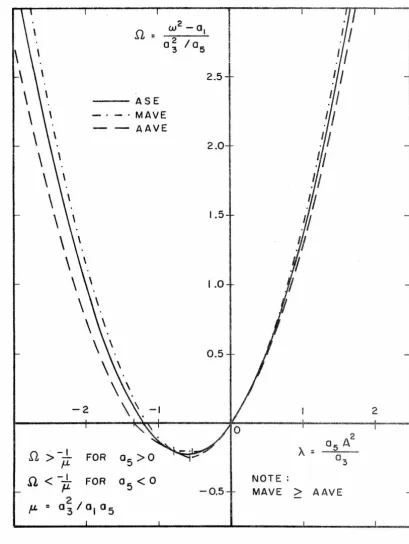
An indication of the accuracy of the cubic approximation may

be obtained by considering some specific examples. Figure l shows

the steady- state response amplitude

f3

as a function of excitation

frequency

w for B

=

0 .1, b

=

0.1, and a= 1 .0. Also shown is the approxi-mation obtained using equivalent linearization. Several exact solution

points were obtained using direct numerical integration of (2. 17), and

these are also included in the figure. It will be noted that the cubic

approximation shows considerable improvement over the usual first

order approximation particularly for frequencies significantly different

from one. This is not surprising since most of the standard solution

techniques require b to be a small number, B to be of order b, and

2

1-w also to be of order b. On the other hand, the accuracy of the

present approach is primarily a function of the magnitude of B and

only indirectly a function of b and

w.

When B approaches zero, the

cubic approximation gives an exact solution of the original system

while the equivalent linearization solution obviously does not. The

b . . t' . . ·1 . - t h b . . (b)

cu ic approxima ion gives simi ar improvemen s w en is negative . Recently, I wan (7) studied Duffing' s

eq~ation

with linear viscous

damping and showed that an equivalent cubic approximation describes

the steady- state behavior much more accurately than the usual

approximation obtained using equivalent linearization.

(30)

CQ

.

w

a

:::> I-_J a.. :E

<I. 5.0

4.0

3.0

2.01

1.0

B=O.I, b=O.I, O=l.O - EQUIV. CUBIC APPROX.

EQUIV. LINEAR APPROX.

• NUMERICAL SOLUTION

/

I

oL~~

0.9 1.0

~~

I.I

~--=~==:::L:=====:r;=====:I;:======Jd

1.2 1.3 1.4 1.5 1.6

FREQUENCY, w

Figure 1: Amplitude versus Frequency for Duffing 1 s Equatio!!

N

(31)

III. ERROR BOUND ANALYSIS

In this chapter, the relationship between the difference of two systems of differential equations and the corresponding difference in their respective solutions is examined. The first section deals with two first order n-dimensional vector systems, and a bound is obtained on the norm of the difference between the two solutions. The second section treats a special subclass of vector systems, namely second order scalar equations, where sharper estimates can be made and better results can be obtained. Sections three and four are devoted to examples which illustrate the use of the theory to obtain bounds for nonautonomous systems (Section 3. 3) and conservative autonomous

system (Section 3. 4).

3. 1. Error Bounds for General Vector Systems.

Before entering into the details of formulating the problem and deriving bounds, it is convenient to introduce some notation which will prove useful throughout the analysis.

Notation

The norm of a vector~· denoted by II~

11

,

is a scalar function that provides a measure of the magnitude of~. A valid norm is any

scalar function of~ satisfying the following conditions:

i) 11~ II~

o •

ii) llxll = 0

n for all~E E , iff x

=

0

(32)

iii) ll~+yll $II~!!

+

11

yl!

iv) llc~ll =

le

I 11~1!

-26-n for all~· y_E: E , for any real scalar c

n and all xE:E ,

(3. l) cont.

where En denotes n-dimensional Euclidean space. Corresponding to each valid vector norm is an associated matrix norm. The norm of a matrix

A,

denoted by

llA II,

is a scalar function that indicates the magnitude of A. A valid vector along with an associated matrix norm satisfy the following relations (2 9):

i)

llA+Bll

s

llAll +II

Bil,

for all nxn matricies

A

and

B,

ii)

II

AB

II

~

II

A II llB

II

for all nxn matricies

A

and B,

11 cA

I

==

lcl llA II

(3. 2)

iii) for any real scalar c and any

matrix

A,

iv) llA~ll ~

llAll II

~11 for any nxn matrix

A

and any vector xEEn ,

It should be noted that the appropriate matrix norm associated with any specific vector norm is not necessarily unique. For any valid vector norm

!12£11,

an associated matrix norm may always be defined by (2 9 )

II A

II =max

II

AJEll,

II

2!:11=1

for all vectors xE:En satisfying

II~!!=

1.

norms and associated matrix norms are: n

i)

11.?Ell

=

l

lxi

I

and i=l

n

II

A

II

== \ '

L

I

a.

lJ

· I i, j =I

(3. 3)

Examples of valid vector

(33)

ii)

11.~11

₌₍

y12

iii) II~

II

=

m~x

I

xi

I

and

l

(Euclidean norm);

(Maximum modulus

norm).

The following analysis is done using general vector and matrix norms,

the only requirement being that they satisfy (3. 1) and (3. 2).

Formulation

Let R be a domain in En and L be the real line. Consider the

problem of finding an approximate periodic solution for the system

dx

-= _d'T

=

F(_{_,}x 'T) (3. 4}

where x and F are n-dimensional vectors,

!'

is pe_riodic with period

T

0 for fixed x,

and£(~,

r) is C

1 _{for ~ER}

and CO for TEL. (Actually,

this condition can be relaxed to F being

c

0 for ~ER and TEL and F

satisfying a modified Lipschitz condition in.x. This point is discussed

in the section on generalizations following the basic analysis.) The

period T

0 need not be the least perio4_ of F(~}T). In general, (3. 4)

possesses a periodic solution with period T

0, but it may also possess

other periodic solutions having periods different from T

0. Assume

that the periodic solution of (3. 4) with period T is of interest. For

s

~{ r) to actually exist, Ts cannot be completely independent of T 0.

Since x('T) has period T , dxd(T) also has period T , and, consequently,

- s 'T s

g~,

'T) is periodic with period Ts. Therefore,

!'

(

~

('T),

'T) =

·

F(

~

(r

}T

8

),

T+Ts)

=.I

(

~

(

T),

'T't-Ts) i.e .

.I( ~

(

T

),

r) is periodic in T for

(34)

-28-fixed x with period T . From above, it rrust happen that T

=

n T 0 for

- s s

n=l,2, ... . If n=l, the solution is called the harmonic solution; the solution having the same period as the least period of the excitation. Inn >-2, the solution is called a subharmonic solution of order n. From the periodicity requirement on .f(~, T). it is clear that there exist no solutions with periods satisfying T

0= j Ts for j=2, 3, ...

Therefore, no periodic solution exists having a period less than the least period of the differential equation. If!'(~, T) is an autonomous system, it possesses all periods in T, and consequently it may possess

solutions with all periods. For example, if there exists a constant vector c such that!'(.£)= _Q, then ~(T) =~is a solution possessing all

periods.

It is possible to obtain an approximate periodic solution by considering an auxiliary system which is represented as

(3. 5)

where a..(i=l, .. ., r) are parameters of the system, y and G are

1 -

-n-dimensional vectors, and G is periodic in T and is

c

1 for _yER and

CO for TEL. It is assumed that (3. 5) has known exact periodic solutions y(f3

1, .. .,f3, T), where f3.(j=l, ... , s) are solution parameters. Since .Y will

- s J

ultimately be the approximate solution, the period of y_ is required to

be the same as the period of the desired solution x. Therefore.

y(T+T ) =:y(T). Depending on the system (3. 5) chosen and on the parti--- s

(35)

pcrh>dic in T with period TA, sur.h that T

8 ., mTi\. for n1 ·:I., or 2, ....

Again TA need not be the least period of G. The equivalent equation

approach may now be used to determine all of the a.(i=l, ... , r) and

1

f3.(j=l, ... ,s).

J

Having found an approximate solution, it is desirable to obtain

son1e indication of its accuracy. For practical purposes, any

com-parison between the exact solution and the approximate solution must

involve only those quantities which are accessible; specifically the differential equations, periodicity conditions, and the approximate

solution. Thus, one is motivated to obtain differences in solutions by considering differences in the corresponding differential equations. To this end, normalize the independent variable T in the following

manner. Since£:'(~, T)..Q(_y, T),~(1") and _y(T) are all periodic with

period T , let s

T

=

tT

s (3. 6)

Then all derivatives with respect to T can be written in terms oft as

d 1

- ( · ) =

dT

T

s d - ( · )

dt

Using (3. 7), equation (3. 4) becomes

dx

-

=

f(x; t)

dt

-(3. 7)

(3. 8)

where

!_5,::_.

t) =Ts!'(~, Tst), and .!J~, t) is periodic int with period 1.

Equation (3. 5) becomes

d_y

_

=

_g(_y,

a

₁, ... ,

ar,

t)

dt

(36)

-30-where

.B

'-'1'

8

~. and .8_ is pe.ri<.>dic int with period 1. It is cl<~a r that .f..

and ~ possess the san1e continuity and differentiability pr ope rtie s as do F and G respectively. The approximate solution

y

is now periodic

in t with period 1.

Denoting the difference between ~(t) and y(t) by x:_(t), th<m

~(t)

=

~(t) -y(t) (3. 1 O)

Differentiating (3. 1 O) and using equations (3. 8), (3. 9) and (3. l 0), the equation for the exact solution error ~(t) is

dz

=

~~+y, t) -

g(y,

t)

dt

(3. 11)

In general, it will not be possible to solve (3. 11) exactly. Therefore,

it seems reasonable to try to obtain a bound on

II

~II in terms of

known quantities, specifically the differential equation error 3t) as

defined by (2. 9). Since ~(t) and _y(t) are both periodic with period l,

~(t) is also periodic with period 1. Therefore, the problem for~ can

be recast in terms of a two point boundary value problem over the

interval 0 :5:t 5: 1 with mixed boundary conditions

~(O)

=

~(l) (3. 12)

The problem for ~(t) then consists of equation (3. 11) subject to the

boundary conditions (3. 12).

In order to proceed further, it is convenient to reformulate

the problem for~ in terms of an integral representation. Consider

(37)

dSQ

=

A(t) _se

dt

SQ( 0 )

=

SQ( l )

(3. 13)

where g?is an-dimensional vector and A(t) is a rum coefficient matrix which is

c

0 int and is chosen such that the only solution of (3.13) is the trivial solution SQ

::

_Q.

A(t) could be the Jacobian matrix

~!(_y,

t) evaluated at the approximate solution

y

if it possessed the above pro-perty of having only the trivial solution. Related to (3. 13) is an Associated Matrix Equation

dZ = A(t)Z

dt (3.14)

where Z is a rum matrix. Let Z(t) be the principal matrix solution of (3. 14) satisfying Z(O) =I, the identity matrix. System (3. 13) will have only the trivial solution if and only if the matrix Q,

Q =Z(O) - Z(l)=I- Z(l) (3.15)

is non-singular. Since (3. 13) has only the trivial solution, it posse se s a Green's function G(t, s) defined as

t

(

t )Q - l Z ( l ) Z -l ( s) G(t, s) =

Z ( t )Q - l Z - I ( s)

, for t< s

(3. 16) , for t>-s,

-1 -1

(38)

-32-Consider now the following inhomogenous problem d_se

dt

=

A(t)SQ

+

j)(t)

(3.17) _se( 0)

=

SQ(l ) '

where A(t) is the same matrix as in (3. 13) and ~(t) is a continuous vector function. Using the Green's function defined in (3. 16), the unique solution of (3. 17) can be written as

1

_se(t)

=

J

G(t, s)§Js) ds 0

(3.18)

The reader interested in proofs of the above statements concerning the existence of the Green's function and the validity of the re presen-tation (3.18) is referred to reference (30).

The problem for ~(t) can now be written as an integral equation. Equation (3. 11) may be written as

d~

*

dt

=

A(t)~+ ~t) + f (~, t) (3. 19)

where A(t) is the same matrix as in (3. 13 ), ~(t) is the differential equation error

~(t)

=

i(y, t) - _g(y, t) ' (3. 2 O)

and

*

(39)

possessed a Green's function . It would be desirable to u::>e this mal-rix for A(t) since all linear terrns in~ would then l.w e liminatcd fron1

.{\~,

t), and, consequently,

II{\~,

t)

II

would be

tjj~

I

as

11~11-o.

Using the Green's function (3. 16) and applying (3. 18), where _:(t)

and{\~.

t) are con side red inhomogenous terms, the integral equation determining

z is

I

~(t)

=

J

G(t,

s)(~Js)

+f

(~(s),

s) )ds 0

(3 . 22)

It is possible to prove the existence of a solution to (3. 22) using the method of successive approximations and, as a consequence, a bound on

ll3!ll

is obtained. These results are presented in the form of

a

Lemma.

Lemma 1

Consider the integral equation (3. 22). If the following conditions are satisfied:

i) ~( s) is a continuous vector function for s E [O, I

J

.

ii)

_{\~(s),

s) is a continuous function of s for sE [O, 1

J

and

of~

for z such that ll~

II

~

o

and satisfies a modified Lipschitz condition of the following form,

jl{~(~

1

(s),

s>-i\~

2

(s),

s)!i

~k(s)\1~

1

(s)-~

2

(s)\I

(3. 23)

for all ~l and ~

2

such that !1~

1

\I ~

o

and 11~

2

ll

~ 5 where k(s) is a positive continuous function of s for s E [O, 1] .

iii) The kernel G(t, s) in (3.22) can be bounded by

(40)

-34-for all tE [O, 1] and sE [O, 1], where p(t) is a bounded non-negative

integrable function for tE[O, 1], and q(s) is a positive continuous

iv)

v)

function for sE [O,

1].

1

K=J k(s)p(s)q(s)ds<l 0

p(t>

I

max

where 5 is defined in ii) and

1

E=

J

q(s>ll£.(s)\\ds 0

Then (3. 22) possesses an exact unique solution ~(t) and

1

\l~(t>ll

$p(t)(l-K)-l

J

q(s)\l.~Js)llds

0

(3 . 2 5)

(3. 26)

(3. 2 7)

Proof: F.xistence of a solution is shown using the method of successive approxiinations. Consider an iteration scheme

z

=

-0

1 1

r

G ( t, s )

~(

s ) d s

Lo

~n

=

~

₀

+

J

G(t,

s){""~n-l(s),

s)ds 0

It is first necessary to show that every iterate satisfies

II

z (t)

II

~ ti

"-n .. n

=

0, 1, ...

(3.28)

(3. 2 9)

(41)

satisfies

li~

₀

(t)

II

$'. p(t) E (3.30)

where E is defined in (3. 26). But since K < 1,

J

!

~

₀

(t)

11

~

p(t)

l (

1-K)-l E

max

(3 .26) implies that 11~

0

(t)\I :s: A. To prove the general case, it is only

necessary to show that

n

ll~n

11 :s; p(t) E ) Ki

i::'O

where K is given in (3. 2 5). Then since K < 1, the pr ope rtie s of n

geometric series may be utilized to show that

l

,

Ki < ( 1-K)- l .

i=O

(3.31)

Consequently,

I

z

I

:s: r, . To prove (3. 31) use induction. Taking norms

. - n

of the second relation in (3. 2 8), 11 z

I

satisfies

- n

Since ~n-l is assumed to satisfy (3. 31), it is permissible to use the

Lipschitz condition (3.23). This, combined with (3.30)and(3.31), gives

1 1

''

~nil

$'p{t)

f,

q{s)1i£(s)!!ds+p(t)

r

q(s)k(s)p(s) •,•

0 0

1 n-1

J

₀

q(r)11

.~,.(r)

II

dr

l

Ki ds i= 0

Combining terms and noting the definjtion of Kand E, llz II is bounded

(42)

as

-36-n

11

~nll

~

p(t) E

l

Ki

i= 0

(3.32)

which is the desired result. Therefore, (3 .32) shows that the use of

the Lipschitz condition (3.23) is valid for any pair of iterates. Before proving that the sequence of functions ~n(t)} is uniformly convergent for tE [O, l], it is necessary to determine bounds on the difference between successive iterates. Consider the difference

z - z

=

-1

-0

l

J

G(t,

s){\~

0

,

s) ds

0

Taking norms and using (3. 23 ), (3. 24), and (3. 32) for n = 0, the above relation becomes

l l

11

~

1

-~

₀

11

~

p(t)

J

0

q(s)k(s)p(s)ds

J

0

q(s)l~(s)\lds

or

11~

1

- ~o II ~ p(t) KE {3.33)

Use induction to show that

(3. 34)

Assume that (3. 34) is va)id for n-1 and consider the norm of ~n - ~n-l . From (3 .28), the difference may be written as

1

ll~n-~n-lll

=

II

J

G(t,s)(l'(~

11

_

1

,s)-

.t

(

~

0

_

2

,

s

))os

\\

(43)

Taking norms under the integral and using the Lipschitz condition and

the bound on G(t, s), the above equation becomes

1

ll~n- ~n-111 ~

p(t)

J,

q(s)k(s)

l~n-1- ~n-211

ds 0

However, by the inductive hypothesis,

Therefore, using the definition of K, the bound on successive iterates

is

Returning to the task of showing that

[z }

_n is uniformly

convergent, consider ~m- Zin for two integers m and n such that rn >n. Writing this difference as a collapsing sum,

m

z _ z

=

I

-m -n ( z . - z .

1 ) -J - J-j=n+l

Taking norms and using the triangle inequality,

m

llz -z

II~\ \~.-z

.

₁11

-m -n

L

J

-:i-j=n+l

Using (3. 34), the above relation becomes

m

II

\'

Kj

11~rn

-

~n ~ p(t) E

L

(44)

-38-But by assumption p(t) is bounded for tE [O, l ] , and K < l which implies that the sequence ~ (t)} of continuous functions converges

n

uniformly to a continuous function .!(t) for tE

[O, 1]

by Cauchy's criterion. ~(t) satisfies (3. 22 ), since the limit as n -+oo can be taken in (3. 2 8). A bound is obtained on j~(t)

II

by taking the limit as n -+oo in (3. 32). Consequently,

l~(t)i

l

~

p(t) (1-K)-l E

Showing that the solution ~(t) is unique is relatively straight-forward. Assume there exists two solutions .!i (t) and ~

2

(t) satisfying

(3. 22), and consider their difference

Since the limit function ?; must also satisfy II~

I

<

8, the Lipschitz

condition (3. 2]) and (3. 24) may be used to obtain 1

llz2-..z.1

II~

p(t)

Jo

q(s)k(s>ll..z.2-£1 lids

Multiplying by q(t), k(t), and integrating, this relation becomes

1 1

J

q(t)k(t)

11.!z -

~

1

lldt s: K

J

q( s )k(s)

\\~

2

-

~

1

\\ ds .

0 0

Since K

<

1, and the integral is non-negative, the only possibility is 1

(45)

Since the integrand is continuous and non-negative, it n1ust vanish

everywhere. But by assumption q(t) and k(t) arc positive for tE [O, 1

J,

therefore

which implies.E.

2 =.E.1 for tE [O, l]. Q .E.D.

In Lemma 1, the integra 1 equation (3. 22) is considered as a.

separate entity. However, in the present analysis, (3 . 22) is related to the differentia 1 system (3. 19). Therefore, the following theorem

applies to system (3. 19). Theorem 1

Let R be a domain in En, and let L be the real line. Consider the original system

dx

df

=

£~,

t)

(3.35) _!(0)=_!(1)

where

.£0f,

t) is

c

1 for

~ER

and

c

0 for tE L, and

il::lf,

t)

=

.£0f,

t+l) for fixed x. Consider also the auxiliary system

d_y

dt

=

_g(y, t)

(3. 36)

.Y( 0)

=

_y( 1 )

where _g(y, t) is C 1 for yE R and c 0 for tEL, and _g is periodic in t with period l £.or fixed :y_. If the difference z is forrned

(46)

-40-then the diffcrentia l system governing~ is

dz ...

d~

=

A(t)~

+

£(t)

+

{'(~,

t)

(3.38)

.

...

where {'<_~, t)

=

!.~+ _y, t)-i_(y, t)-A(t)~, £(t)

=

i_(_y, t)-_g(y, t) , and A(t) is a continuous matrix function oft. If the homogenous problem

d'.SQ

-- = A(t)rn

dt ..::t:

_sp( 0)

=

_sp( I )

(3. 3 9)

has only the trivial solution, it possesses a Green's function defined by (3.16). Furthermore, if

,..I

K

=

J

k(s)q(s)p(s)ds <l 0

(3.40)

(Q and Z are defined in (3 .14) and (3 .15) ), and k(s) is a Lipschitz

...

constant for{'·(~, t), an<l if

p<t>

I

(1-K)-l Es: 5 , (3. 41)

max 1

where E=

J

q(s)il£(s)lids and 5 defines a region

11.~l

l:-;;;

5 for which

..._ 0

{'"(~. t) is Lipschitzian, then the following conclusions may be reached. The original system possesses an exact unique periodic solution for ~ER. Furthermore, the norm of the error ~(t) can be bounded as

(47)

>:-:

If, in addition, .!_ ~. t) satisfies

max

I

M;

*

(~,

t)

JI

~

k(t) 1~11~ f,

(3 . 43)

the exact unique solution ~(t) is an isolated solution. (An isolated

periodic solution~ is one such that the equation of first variation

associated with it possesses no non-trivial solution with the same

period as~·)

Proof: Differentiating (3.37) and using (3.35), (3 .36), and (3.37), the

governing equation for ~(t) is found to be dz

dt = .!_(~+ Y.• t) - g(y, t)

~(O)=~(l) .

Adding and subtracting A(t)~+i_(y_, t) to the right hand side, (3. 38) is

obtained. However, by assumption, the homogenous problem (3 .3 9)

possesses a Green's function. Therefore, by (3 .18), the error z

satisfies ₁

~(t)

=

J

G(t,

s)(~(s) +i_*(~(s),

s))ds 0

where G(t, s) is

{

~(t)Q-l

Z(l)Z-l(s)

G(t,s) = I l

Z(t)Q-

z-

(s)

, for t< s

, for t:<:: s

(3. 44)

Z(t) is the principal matrix solution of (3. 3

9),

and Q is a non-· singular

matrix given by Q =I - Z(l).

Define

p ( t) =

II

Z ( t)

11.

q ( s ) = max (

II

Q - 1 Z ( I ) Z - 1 ( s )

II

. II

Q - 1 Z ( s )

II )

.

(48)

-42-will also be continuous. Since.£~. t) is continuously differentiable with

""

respect to

.?E•i

(~, t) will also be continuously differentiable in~·

~\:

Therefore, for all II~

II:<.;;

& ,

i

(z,

t) will satisfy a modified Lipschitz condition of the form

.,

11.£\~2'

t) -

{

-:<

(~

l' t)

II

~

k(t)

11~2

-

~I

Ii

where k(t) is continuous and positive for tE [O, l]. Using assumptions

(3. 40) and (3 . 41), it is clear that all of the hypotheses of Lemma l

a.re satisfied, and consequently, (3. 44) has an exact unique solution

z;(t) with

I

z(t)

I

~

p(t) (1-Kf 1 E

Since (3. 44) has an exact unique solution, (3. 3 5) must also possess an exact unique solution. Since the solution of the original system is

~ =_y+~ where

.Y

is a known prescribed function, ~(t) existing and being

unique implies that ~(t) exists and is unique.

To show that x is an isolated solution, if (3. 43) is satisfied, is straightforward. Consider the equation of first variation of (3. 3 5),

d5

8f (x, t)

dt :::~- ~ (3. 4 5)

Adding and subtracting A(t) S,_ to the right hand side, the representation (3. 18) can be used to obtain

5(t) =

f

G(t, s>[

¥x(~(s),

s) -A(s) ]5(s)ds

0

-(3. 46)

(49)

From (3. 3 7) .and (3 . 3 8 ),

.D.?E·

t) may be written as

f_(~.

t) =

{\.~-_y,

t) + i_(_y, t) + A(t) (.?E+ _y)

Noting that

l'(~,

t) is continuously differentiable, the Jacobian matrix

may be formed yielding

8f (x, t) 8f ~:.!

8x

=

Tz

(.?E-.Y• t) +A(t)

Taking norms of (3. 46) and using the above relation, s(t) satisfies

I

ll~(t)ll

,;;; p(t)

J

q(s)k(s)ii~Js)

l

ids

0

where it is assumed that llx-y

II

s 5 so that the use of (3. 43) is justified.

Multiplying by q(s) and k(s) and integrating, the above relation becomes,

I

(1-K)

l

q(s)k(s>ll.S.Js)llds s O, tJO

where the definition of K has been used. Since K < l and the integral

is non-negative, the only possibility is that the integral must vanish.

Since the integrand is assumed continuous for tE [O, l], and q(s) and

k(s) are positive, the above relation implies that

Therefore, the exact periodic solution x of the original system (3 .3 5)

is isolated. Q. E. D.

It is also possible to prove the following.

Theorem 2

(50)

-44-periodic solution~ with period I. Then for any smal1 number f), it

is always possible to choose an auxiliary system (3. 36) with an exact

periodic solution y such that the differential equation error is

sufficiently sma 11 so that the norm of the difference between~ and y

satisfies 11~-y

II :;;

o

·

Proo!.'... Consider the integral equation

where .§.(s) = µ ~(x(s), s) and~ is continuously differentiable in~ for

sE[O, l] and

*

of

£

(~(s), s) =:!_(~, s)-£(~-~· s)- ~(~, s) z

µ(_g_(~,

s) -

_g(~-~·

s))

. of

G(t, s) is the Green's function for the system (3. 39) with A(t)

=

₀

;(~, t)

which exists since the equation of first variation possesses no

nontrivial solution with period 1, i.e. ~ is isolated. For ~

1, ~

2

, and

µ satisfying 11~

1

11 :;;

11

:;;

5, 11~

2

11::;;

11 :

;

5, and

Iµ I :;;

µ

1 where 'lland µ1 are sufficiently small positive numbers,_!::!'(~, s) satisfies a modified

Lipschitz condition,

such that max k(t) can be taken to be as small as desired. Select T) t

and µ

1 sufficiently small such that k(t) may be chosen small enough so

(51)

bounds on G(t, s). Furthermore, let

1-lz

be the small positive number

such that for Iµ I $µ 2,

I

II

lu lp(t)I (1-K)- q(s) Ii.&(~-· s)

II

ds $'Tl

max 0

Then, for 11~11 :;;;T) and Iµ 1$ min(µ₁, _{µ 2 ), all the conditions of Lemma}1

are fulfilled. Therefore, the above integral equation possesses an

exact unique solution such that 11~11 ~ri ~ 5.

However, it is shown previously that the integral equation is

equivalent to the differential system dz 8f (x, t)

dt

=

ii-

~+ £!'(~. t)

+

~(t)

~(O) =~(I)

Using the definitions of ~(t) and.!.""(~, t), the system becomes,

dz

d~ =£(?Er t) -_!(_?E-~, t) +µg_(_?E-~, t)

Subtracting this system from the original system (3. 3 5) and defining

y

=~-~· one has

dy

dt

=

.!_(y,

t) -

1-1_g(y,

t)

,y(O)=y(l) .

For Iµ I$ min

(1-1

1, µ2), the above system possesses an exact unique solution of period .I such that 11~-yil ~ 5. Therefore, the above systcrn

(52)

5 represents a bound on the error which is uniform in t.

Usually it is desirable to obtain the smallest bound possible, therefore the equality sign is used in equation (3. 41) for determining

o.

Generalizations

Some of the hypotheses in Lemma 1 and Theorem 1 can be weakened to include more general systems. The condition that f(~, t) be

c

1

in~

can be replaced by assuming that !J:E., t) is

c

0 in :E. and

$atisfies a modified Lipschitz condition in~· The proofs of Lemma 1 and Theorem 1 are only slightly modified with the exception that in Theorem I it is no longer possible to conclude that the exact solution is isolated since the equation of first variation is not defined.

The assumption in Lemma 1 that q(s) and k(s) be positive continuous functions for sE [O, I] can be weakened to q(s) and k(s) being non-negative, integrable functions for s E [O, 1

J

with the loss of "strict" uniqueness. It is possible to conclude only that if there exists two solutions to (3.22), ~l and~

2

, then

Therefore, the integrand vanishes everywhere except at a set of points with zero measure. For all values oft where k(t)q(t)> 0,

11!!.

₁- ~

2

11 is zero, which implies ~l

=

~

2

. Consequently, uniqueness is obtained only over a subset of tE[O, l].

Autonomous Systems

(53)

conditions are satisfied, the equation of first variation of the original syste1n associated with the exact periodic solution ~(t) possesses no

non-trivial solution with the same period as x.(t). However, for auto-nomous systems it is well known that, if the original system possesses a non-trivial periodic solution ~(t), the equation of first variation

dx(t)

associated with x(t) has a non-trivial periodic solution

a";

with the same period as ~(t). In this situation, hypothesis (3. 40) in

Theorem 1 can never be satisfied. Consider the following autonomous

system

dx

_:: = f(x)

dt - - (3. 47)

Assume .. H~) is continuously differentiable with respect to x and that the Lipschitz constant k( s) for i*(~. t) satisfies (3. 43). Differentiating

with respect tot, (3. 47) becomes

_E_(

~)

=

8f(#$'.) ~

dt dt 8x dt (3. 48)

Assume that (3. 47) possesses a non-trivial periodic solution with

dx

period 1. Then, dt will also be periodic with period 1 and will satisfy the equation of first variation (3. 48). Adding and subtracting

dx

A(t) d-: to (3. 48), where A(t) is the same matrix that appears in

t dx

(3. 3 9), and writing this modified equation in integral form, dt satisfies

dx

Jl

[

Sf(x)

J

d~

dt - G(t, s)

-rx-

-

A(t) dt ds

0

(3. 49)

(54)

-48-satisfies

_i'!<(~-_y, t)

=

_!J~) - _!_(_y) - A(t)(~+_y) (3. 50)

where :y_ is some periodic function such that for~= .!E,-y,

.£>:

'

(,;,

t) satisfies a modified Lipschitz condition given in (3.23) for ll~ll::;;o . Forming the Jacobian matrix for f.>1'~-y, t)

of*(x-y, t) 8f(x)

Bx

=

Bx

-A(t) (3.51)

Taking norms of (3.49) and using (3 . 51) and the bound on llG(t, s>ll dx

given in (3. 24),

II

dt

II

satisfies

dx 1 dx

lldtll::;;p(t)

J

q(s)k(s>lld~llds,

0

(3. 52)

where it has been assumed that 11~-yll:::;; o so that use of (3. 43) is justified. Multiplying by q(t) k(t) and integrating, the above relation

1 dx

(1-K)

J

q(t)k(tllldt i!dt::;;O,

0

dx

where the definition of K has been used. But if

Equivalent differential equations for nonlinear dynamical systems

ACKNOWLEDGEMENTS

ABSTRACT

TABLE OF CONTENTS

COMPARISON OF VARIOUS EQUIVALENCE CRITERIA

TECHNIQUES 186

-II. EQUIVALENT EQUATION APPROACH

w for B

eq~ation

EQUIV. LINEAR APPROX.

llA II,

AJEll,

q(s)\l.~Js)llds

0

0

0

0

0

0

0

0

q(s)l~(s)\lds

0

0

q(s)k(s>lld~llds,

₀

₀

₀

₀

₀

₀