Numerical Relativity beyond General Relativity

(1)

Thesis by

Maria Okounkova

In Partial Fulfillment of the Requirements for the Degree of

Doctor of Philosophy in Physics

CALIFORNIA INSTITUTE OF TECHNOLOGY Pasadena, California

2019

(2)

Maria Okounkova ORCID: 0000-0001-7869-5496

(3)

Space may be the final frontier but it’s made in a Hollywood basement

(4)

ACKNOWLEDGEMENTS

I have many wonderful colleagues to thank for the work presented in this thesis.

Thank you to Saul Teukolsky, my advisor, for all of the physics discussions we have had over the years. Your suggestions and advice are always helpful.

Thank you to Mark Scheel, for teaching me about numerical relativity, and patiently

answering questions about code.

Thank you to (Professor!) Leo Stein, for motivating me to delve deeper into theory.

Thank you to Daniel Hemberger, for all of the work that you have put into developing a good, working code, and for your ever-inspiring coding practices.

Thank you to Swetha Bhagwat, for being an amazing co-author.

Thank you to the other members of the Simulating eXtreme Spacetimes (SXS)

collaboration, for all of your help over the years. Thank you to my additional

coauthors, Matthew Giesler, Duncan Brown, and Stefan Ballmer.

Thank you to my committee members, Rana Adhikari, Yanbei Chen, Sergei Gukov,

(5)

ABSTRACT

Einstein’s theory of general relativity has passed all precision tests to date. At some

length scale, however, general relativity (GR) must break down and be reconciled

with quantum mechanics in a quantum theory of gravity (a beyond-GR theory).

Binary black hole mergers probe the non-linear, highly dynamical regime of gravity, and gravitational waves from these systems may contain signatures of such a theory.

In this thesis, we seek to make gravitational wave predictions for binary black hole

mergers in a beyond-GR theory. These predictions can then be used to perform

model-dependent tests of GR with gravitational wave detections.

We make predictions using numerical relativity, the practice of precisely numerically

solving the equations governing spacetime. This allows us to probe the behavior of

a binary black hole system through full inspiral, merger, and ringdown. We choose to work in dynamical Chern-Simons gravity (dCS), a higher-curvature beyond-GR

effective field theory that couples spacetime curvature to a scalar field, and has

motivations in string theory and loop quantum gravity. In order to obtain a

well-posed initial value formalism, we perturb this theory around GR. We compute the

leading-order behavior of the dCS scalar field in a binary black hole merger, as well

as the leading-order dCS correction to the spacetime metric and hence gravitational

radiation. We produce the first numerical relativity beyond-GR waveforms in a

higher-curvature theory of gravity.

This thesis contains additional results, all of which harness the power of numerical

relativity to test GR. We compute black hole shadows in dCS gravity, numerically

prove the leading-order stability of rotating black holes in dCS gravity, and lay out

a formalism for determining the start time of binary black hole ringdown using

(6)

PUBLISHED CONTENT AND CONTRIBUTIONS

[1] Maria Okounkova, Mark A. Scheel, and Saul A. Teukolsky. “Evolving Metric Perturbations in dynamical Chern-Simons Gravity”. In: Phys. Rev. D99.4 (2019), p. 044019. doi: 10.1103/PhysRevD.99.044019. arXiv:

1811.10713 [gr-qc].

M.O. conceived of the project, performed the analytical calculations, wrote the code, performed the simulations, analyzed the data, and wrote the manuscript.

[2] Maria Okounkova, Mark A Scheel, and Saul A Teukolsky. “Numerical black hole initial data and shadows in dynamical Chern–Simons gravity”. In: Clas-sical and Quantum Gravity 36.5 (Feb. 2019), p. 054001. doi: 10.1088/ 1361-6382/aafcdf.

M.O. conceived of the project, performed the analytical calculations, wrote the code, performed the simulations, analyzed the data, and wrote the manuscript.

[3] Swetha Bhagwat et al. “On choosing the start time of binary black hole ringdowns”. In: Phys. Rev. D97.10 (2018), p. 104065. doi: 10 . 1103 / PhysRevD.97.104065. arXiv:1711.00926 [gr-qc].

M.O. conceived of the project jointly with S.B., and the two wrote the code, performed the analytical calculations, performed the computations, analyzed the data, and wrote the manuscript.

(7)

INTRODUCTION

1.1 A century of general relativity

Over one hundred years ago, Albert Einstein put forth the theory of general relativity

(GR), coupling spacetime to the matter and energy contained within [82].

In the century following this discovery, there was much progress in exploring the

properties of this classical theory. The theory was found, for example, to contain

black hole solutions [180]. Later, it was discovered that the theory contained

spinningblack hole solutions [112,197]. Swiftly, scientists began to think not only

about single black holes, butbinaryblack hole systems. In binaries, two black holes

orbit one another, inspiraling closer together through the emission of gravitational radiation, and ultimately merging in a violent, energetic process, to form one black

hole. Theoretically computing the gravitational radiation (or gravitational waves)

emitted by binary systems was of particular interest [135, 156]. The end of the

century saw the first precise, numerical prediction of a full gravitational waveform

from a binary black hole merger [161].

1.2 Gravity beyond general relativity

The same century, however, saw the development of quantum mechanics and

quan-tum field theory as a description of nature. If the universe is ultimately quanquan-tum,

then general relativity, a classical theory, does not fit into this picture as an

appropri-ate theory of gravity. From a quantum field theory standpoint, general relativity is

non-renormalizable. This means that in order to perform a perturbative expansion of GR, one needs an infinite number of parameters (unlike, for example, quantum

electrodynamics, which requires only a few parameters, such as charges and masses).

This in turn led to various efforts to come up with aquantum theory of gravity. Such

a theory would behave like general relativity at low energies (much like general

relativity reduces to Newtonian gravity at low energies), but contain quantum effects

at high energies. The most notable candidates for a theory of quantum gravity are

string theory and loop quantum gravity. In string theory, in contrast to ordinary quantum field theory, the fundamental object is a one-dimensional string, rather than

(10)

to a given mode of a string (cf. [41]). Loop quantum gravity, on the other hand,

quantizes space and time, so that spacetime is no longer a classical field, but rather discrete at the Planck length,∼10−35meters (cf. [174]).

When considering physical theories, we must think about testable predictions. Since

we know general relativity breaks down at high energies, let us consider predictions

for astrophysical systems in the strong-field, dynamical regime of gravity, such as the merger of black holes.

Were we to directly work in a full quantum theory of gravity, these calculations

would quickly become prohibitively complicated, if one could even formulate how

to do them at all. Instead, we can work in effective field theories. These modify the Einstein-Hilbert action of general relativity, through the inclusion of classical

terms that encompass high-energy quantum gravity effects, to produce a beyond-GR

theory.

Beyond-GR effective field theories, thus, are valid at intermediate ranges, as they account for some high-energy effects, but not all, by virtue of being truncations at

some energy. Astrophysical systems that probe the strong-field regime of gravity,

such as binary black hole mergers, could potentially contain beyond-GR effects in

this intermediate range.

Let us begin looking at the form of some beyond-GR effective field theories, by

considering their (classical) actions. Let us start with the standard Einstein-Hilbert

action of general relativity, which we will write as

S = 1

16π ∫

d4x√−gR, (1.1)

wheregabis the spacetime metric,gis its determinant, andRis the spacetime Ricci

scalar. Beyond-GR theories will modify this action, whether by adding more terms

or changing the form of theRterm.

One class of effective field theories of gravity arises from considering actions with

higher-order curvature terms added to the Einstein-Hilbert action. In this picture,

general relativity becomes a lowest-order term in an action expanded in powers of

all possible curvature invariants. In particular, let us focus on terms quadratic in

the curvature (the leading-order correction). Adding quadratic-curvature terms to

the Einstein-Hilbert action makes it renormalizable [186], thus solving our original

problem. Of particular interest are the combinations

∗

(11)

known as the Pontryagin scalar, and

R_GB2 = R2−4RabRab+RabcdRabcd, (1.3)

known as the Gauss-Bonnet scalar. Both scalars appear in low-energy realizations

of string theory [157, 18], and the Pontryagin scalar additionally appears in

loop-quantum gravity [192, 134]. Hence, these are motivated byunderlying theories of

quantum gravity.

Coupling these quadratic curvature invariants to a scalar fieldϑ creates a class of quadratic gravity theories, including Einstein-dilaton-Gauss-Bonnet gravity, with

the action

S= 1

16π

∫ _√

−gd4x R−2∇aϑ∇aϑ−V(ϑ)+αf(ϑ)R_GB2 , (1.4) for some coupling function f(ϑ) and potential V(ϑ). Here, the first term is the familiar Einstein-Hilbert action of general relativity, the second and third terms

correspond to a canonical stress-energy tensor for the scalar field, and the last term couples the scalar field to the Gauss-Bonnet spacetime curvature scalar. The quantity

α1/2_{, meanwhile, is a coupling parameter with dimensions of length that determines}

the truncation of the effective field theory – the length scale below which quantum

gravity effects become important.

Similarly, we can obtain dynamical Chern-Simons gravity, with the action

S= 1

16π

∫ _√

−gd4x R−2∇_aϑ∇bϑ−V(ϑ) −`2ϑ∗RR. (1.5) Here, the fourth term couples the scalar field to the Pontryagin curvature quantity. The quantity` in this case is a coupling parameter with dimensions of length that similarly denotes the length scale below which quantum gravity effects become

important.

These theories contain terms motivated by full quantum gravity theories (namely

string theory and loop-quantum gravity), and hence serve as classical

approxima-tions to some underlying quantum theory of gravity, truncated at second-order in

curvature. One can, in theory, perform the same calculations outlined in Sec. 1.1

for these beyond-GR theories. Namely, one can make predictions for black hole

metrics, perturbations to these metrics, and the behavior of binary black holes.

1.3 Testing general relativity in the strong-field regime

These physical theories, however, are nothing without experimental evidence, and

(12)

astrophysical observations [206]. Recall that we aim to test general relativity in the

strong-field, towards a regime where quantum gravity effects could be important.

The strongest tests of general relativity were previously given by binary pulsar

systems, including the notable Hulse-Taylor Pulsar, PSR B1913+16 [106]. These

tests found consistency with Einstein’s quadrupolar formula for gravitational wave

emission at a 0.1% level and placed bounds on dipolar radiation, which does not occur in pure GR [205,43].

However, binary pulsar observations are relativelyweak-fieldcompared to, for

exam-ple, the merger of black holes and neutron stars, which at once probe the largest

grav-itational potentials and highest curvatures of any available astrophysical system (cf.

Fig. 1 of [37]). Indeed, attempts to map binary pulsar observations onto constraints

on quadratic gravity theories produce a relatively weak theoretical bound [214,212].

It would take a century after the advent of general relativity to probe gravity in the

strong-field regime. In 2015, the Laser Interferometer Gravitational-Wave

Observa-tory (LIGO) made the first detection of gravitational waves from a binary black hole

merger [10], probing the strong-field, dynamical regime of gravity for the first time.

Together, LIGO and its sister detector, Virgo, have detected gravitational waves from

ten binary black hole mergers in the O(1−100)M range, and one binary neutron star merger [9, 8], with more detections at even higher experimental sensitivity on

the way [3,13].

Testing general relativity with gravitational wave observations: present

How can one test general relativity with gravitational wave observations? To look at the state of the art, let us turn to some of the tests in [14], the companion analysis

testing general relativity for GW150914, the first LIGO detection [10].

One of the first tests one can perform is a simplenull test, by checking the consistency

of the null hypothesis (GR in this case) with the data. For GW150914, the

most-probable GR waveform [12] was subtracted from the gravitational wave data from

each detector, leaving a residual signal. If some loud, non-degenerate, unmodeled

deviation from GR were present in the detected gravitational wave, then it would show up as a coherent signal between the two detector residuals. If, however,

there were no deviations from GR, the residuals should contain only (uncorrelated)

noise [70]. The residuals for GW140915 were not statistically distinguishable from

noise, verifying the GR prediction for GW150914 to 4% [14].

(13)

detected waveform. In general relativity, by the so-called no-hair theorem, (vacuum,

asymptotically flat, stationary, axisymmetric, uncharged) black holes are completely characterized by just two parameters – their mass and spin [132,135,76,94, 111].

In GR, after a binary black hole merger, the resulting single black hole enters the

ringdown stage, where its gravitational wave spectrum is described by a linear

superposition of damped sinusoids, known as quasi-normal modes (QNMs), which

are paramterized by a damping timeτ and frequency ω. By the no-hair theorem, these modes (in GR) purely depend on the mass M and spin χ of the final black hole. That is,

(

χ M

)

↔

(

ω τ

)

. (1.6)

In some beyond-GR theories, however, black holes have additional hair – that is,

there are additional parameters characterizing the ringdown stage and final remnant

beyond the mass and spin. In this case, the QNM spectrum will differ from that

predicted by GR.

While rigorously checking ringdown consistency with GR requires observing at

least two modes for a given signal [94, 111], a weaker test was performed with

GW150914 in [14], with just one mode. First, the most-probable GR waveform matching just the inspiral part of the gravitational wave signal was found. From

the binary black hole parameters of this waveform, one can theoretically compute

what the final mass and spin of the remnant black hole should be in GR [102,

201]. This mass and spin will then give unique predictions in GR for the damping

time and frequency of the ringdown QNM spectrum. Thus, one can perform a

consistency check between these theoretically predicted QNM parameters, and the

QNM parameters measured by fitting damped sinusoids to the post-merger part of

the detected signal. For GW150914, the 90% credible regions for the measured

QNM parameters and the predicted QNM parameters for one mode overlapped, thus showing compatibility with GR. Such a test is also anull test, in that it checks the

consistency of the signal with GR predictions (the null hypothesis), rather than using

predictions for ringdown behavior from other, competing theories.

In addition to null tests, there are parametrized tests of general relativity one can

perform with gravitational wave observations. In this case, the gravitational wave

(14)

GR. For example, in the Parametrized Post-Einsteinian (ppE) formalism [215, 71],

the functional forms of the amplitude and phase of the gravitational wave signal are modified, and include some additional parameters. In [216], the authors used the

ppE framework on GW150914 data to constraint various ppE parameters (and hence

departures from GR). One can also modify the analytical form of the Post-Newtonian

(PN) expansion, which describes the inspiral part of the gravitational wave signal.

Extra terms (with extra parameters) are added to each order of the expansion (either

one order at a time, or all together). In the LIGO GW150914 testing GR paper[14],

the authors tested such a modified PN expansion against GW150914 data, finding

no consistent departure from GR. These tests, however, only modify the inspiral

part of the waveform, without considering the more-energetic merger phase.

In [15], the LIGO and Virgo collaborations used all of the LIGO and Virgo events [9]

to test general relativity. In particular, they repeated the null test of subtracting the

best-match waveform, and checking that parametrized deviations in PN coefficients

were zero.1 The data was not inconsistent with the predictions of GR, and constraints on deviations from GR decreased by a factor of∼2.

Testing general relativity with gravitational wave observations: future

possi-bilities

We can in theory perform stronger tests of gravity than null and parametrized tests

of general relativity. What if, in addition to best-match gravitational waveforms in general relativity, we had access to best-match gravitational waveforms in a

theory beyond general relativity, such as dynamical Chern-Simons gravity? Then

we can perform parameter estimation using the method currently used for general

relativity [12] to find the best-match waveform in dynamical Chern-Simons gravity.

In particular, dCS has an additional parameter,`, which can (in theory) be measured. This match can then be compared to the match one gets with pure GR, using Bayesian

model selection.

Parametrized tests, in a sense, do use a beyond-GR model. However, the merger regime in this case is not well understood. In fact, in [216], the authors discussed

the theoretical implications of the GW150914 detection, including a ppE analysis,

and argued that “the true potential for GW150914 to both rule out exotic objects

and constrain physics beyond General Relativity is severely limited by the lack of

1_{There is a wealth of other tests of general relativity that can be performed with gravitational}

(15)

understanding of the coalescence regime in almost all relevant modified gravity

theories."

A stronger test of gravity with gravitational wave observations then would require

the use of gravitational waveforms in a beyond-GR theory.

Let us now discuss how to generate such beyond-GR waveforms. If we wish to

perform an analysis with the same level of precision and accuracy as GR analyses,

then we need access to waveforms of comparable accuracy. The most accurate grav-itational waveforms [2,1] come from numerical relativity, the practice of precisely

solving the non-linear, highly-coupled partial differential equations governing the

behavior of spacetime.2 Binary black hole numerical relativity simulations, however can take on the order of weeks or months to compute. In order to find a best-match

waveform as in [14,12], data analysts must go through millions of waveforms. To

produce a numerical relativity simulation for each on a short timescale would be

infeasible. Thus, numerical relativity waveforms are used to calibrate waveform

models that are faster to evaluate, including the Effective-One-Body model [191]

used in [14,12]. There is also growing interest in gravitational wave data analysis surrogate models, waveform models with NR level accuracy that are trained on

NR waveforms [118, 49]. In each of these cases, however, we must first produce

numerical relativity gravitational waveforms.

Our goal, thus, is to produce numerical relativity gravitational waveforms in a

beyond-GR theory of gravity. This is the main topic of this thesis.

1.4 A brief introduction to numerical relativity

As stated before, numerical relativity (NR) is the practice of precisely solving the

non-linear, highly coupled partial differential equations governing the behavior of

spacetime. Without going into too much technical detail, let us take some time to

give a brief overview of the subject. For an excellent primer on NR, see [40]. We

will focus on numerical relativity in general relativity for now.

In analytical relativity, spacetime is characterized by a 4-dimensional spacetime

metric, gab. General relativity is a covariant theory, in which all expressions,

such as the Einstein field equations, hold true in any coordinate system [203, 64].

Spacetimes such as the Kerr and Schwarzschild black hole solutions are written

2_{Throughout this thesis, we use precisely this definition of numerical relativity. Some sources}

(16)

down in terms of 4-dimensional coordinates, often containing the full dependence

on a time coordinate,t[203].

In numerical relativity, we are interested in situations where the full 4-dimensional

spacetime is unknown. It is difficult, for example, to write down the entire spacetime

of two merging binary black holes. Instead, in NR, we start with some initial

conditions and evolve a spacetime. For example, we start with two black holes sitting far apart from each other, and evolve this configuration to see what happens

with time.

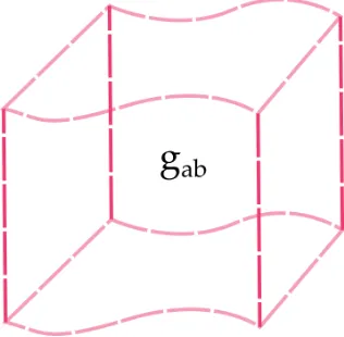
In this picture, the 4-dimensional spacetimegabis decomposed into spacelike and

timelike pieces. Namely, a 4-dimensional spacetime is foliated by a set of spatial

slices {Σ_i}. The normal vector na to each spatial slice is timelike, and we use this vector to move in time from slice to slice. Each slice Σi is labeled by some

coordinate time,ti. On each sliceΣ of a spacetime with spacetime metricgab, the

timelike normal vectornainduces a spatial metric onΣ,γab, as

γab= gab+nanb. (1.7)

We illustrate this picture in Fig.1.1.

(a) Spacetime as seen by an analytical relativist (with one spatial dimension suppressed).

(b) Spacetime as seen by a numerical rel-ativist (with one spatial dimension sup-pressed). The unit timelike normal vec-torna is shown schematically here, for one point on one slice. These is such a vector for each point on each slice.

Figure 1.1

Now that we have sliced up the spacetime, let’s think about the form the Einstein

(17)

(ADM) equations [28]. The equations take the form of two elliptic constraint

equations that the metric must satisfy on each sliceΣi, and twohyperbolic evolution equations governing how the metric data evolves from slice to slice. Satisfaction

of the constraints means that the evolution is precisely solving the Einstein field

equations.

In order to perform a simulation, we generateinitial datafor the metric (and its first

derivatives) on an initial sliceΣ₀by solving the elliptic constraint equations. Then, these data are evolved using the hyperbolic evolution equations to obtain the metric

on all subsequent slices. We show this schematically in Fig.1.2. This constitutes

the “simulation", and gives us the results.

Figure 1.2: Schematic of initial data and evolution formalism.

However, performing this evolution is not so simple. In order to have a stable evolu-tion, we must have awell-posed initial value problem. In this case, given an initial

solution to a partial differential equation at some time, the solution cannot grow

faster than exponentially. This is especially important in the context of numerical

relativity, in which the numerical solutions to partial differential equations always

have some level of numerical noise. What we want to guarantee is that if we add

some numerical noise to an initial condition, we will not get a completely different

solution to the problem at some later time.

The 3+1 ADM equations, however, are not well-posed, and performing an evolution

using these equations will lead to numerical blow-up. It took some time to formulate

the equations of general relativity in such a way as to guarantee that the initial value

problem was well-posed. Some popular such formulations are the harmonic and

generalized harmonic formalisms [67, 88, 162, 161, 121]. Indeed, it took almost

(18)

merger to be successfully performed [162,161], mainly due to choosing appropriate

evolution equations.

Recall additionally that the equations of general relativity are independent of the

choice of coordinates. However, when performing a numerical simulation on a

computational domain, we must specify a coordinate system. In particular, though

GR as a theory is gauge invariant, we must specify a gauge for our numerical

simulations. This leads to another complication – one must choose a satisfactory

gauge in which to work [40].

Binary black hole simulations have their own unique challenges, beyond choosing

appropriate evolution formulation and gauge. For example, we must determine

how to numerically deal with the black hole singularities [104]. Additionally,

while it is relatively simple to construct a computational grid for one stationary

black hole, it is not so simple to a construct a grid that will faithfully be able to

resolve two rapidly moving, merging black holes [179]. We must likewise have

methods to find the black hole horizons numerically during a simulation (if desired

or required) [98, 68, 53]. Finally, if the ultimate goal of a binary black hole

simulation is to produce a gravitational waveform prediction, we must have methods for extracting this radiation [193,56].

1.5 Pushing numerical relativity beyond general relativity

How does the picture of numerical relativity put forth in Sec. 1.4 change when

we work not with general relativity, but a beyond-GR theory? Let us focus, as in

this thesis, on a particular 4-dimensional theory of spacetime, namely dynamical

Chern-Simons gravity.

We still foliate the spacetime into spatial slices as in Fig. 1.1. The 3+1 ADM

equations, however, are equations for general relativity. We thus need to derive a set

of constraint equations for initial data and evolution equations in dCS. However, it is believed that dCS doesnothave a well-posed initial value problem [74]. We thus

cannot perform simulations of spacetime in the full dCS theory.

However, we know from Sec. 1.3 that deviations from general relativity, in the

regime observable by gravitational waves, must be small. Thus, we can work

perturbatively around GR, and perturb the equations governing dCS around an

arbitrary GR solution, such as a binary black hole background. We expand both the

spacetime metric and the dCS scalar field in powers of the coupling parameter, and

(19)

scheme.

The key to the order-reduction scheme is that GR is a quasilinear theory: the

high-est derivatives of the metric appear linearly in Einstein’s equations. Accordingly,

at each order in perturbation theory, the equations have the same principal part

(leading-order derivative terms) as in general relativity. The principal part

deter-mines whether the equations have a well-posed initial value problem. Since we know

how to formulate GR in a well-posed way, we can do the same for the order-reduced

dCS equations, and obtain a well-posed evolution scheme.

At zeroth order in the coupling, we recover general relativity. At first order in the

coupling, we see our first dCS correction to GR, namely in the scalar field dynamics.

The GR background sources a leading-order dCS scalar field. At this order, there

is no dCS modification to the metric. At second order, the GR background and

the first-order dCS scalar field source a leading-order dCS metric perturbation. It

isthisfield we are after, as it will give us the leading-order dCS modification to a

gravitational waveform. We illustrate this system in Fig.1.3.

In order to generate the leading-order dCS corrections to a binary black hole

wave-form, we must first be able to evolve a binary black hole system in GR (zeroth order).

This problem has long been solved [2,1]. However, we must now begin to add dCS

modifications to the system.

Evolving the leading-order dCS scalar field

In order to obtain dCS corrections to the spacetime metric (and hence the

gravi-tational waveform), we must first evolve the leading-order dCS scalar field, which sources this correction. This is the main objective of Chapter2of this thesis, where

we develop a formalism and code to evolve the leading-order dCS scalar field on an

arbitrary GR background.

We consider a variety of binary black hole systems with spin and compute (scalar)

waveforms for the scalar field. The dominant radiation pattern of the scalar field

during inspiral is quadrupolar, and we find good agreement with PN theory

pre-dictions for the inspiral phase [212]. However, unlike in PN theory, we evolve the system through merger and ringdown. In particular, we find a burst of dipolar scalar

radiation at merger, a hitherto unknown phenomenon.

We use the scalar field to estimate the strength of the leading-order dCS correction

to thegravitationalradiation. We find that were LIGO to detect a GW150914-like

(20)

(21)

be bounded by` _.O(10)km, a result eight orders of magnitude stronger than that from solar-system tests [20].

Initial data for leading-order dCS spacetime metrics

If we wish to evolve the leading-order dCS metric perturbation sourced by the scalar

field, we must first generate initial data for this metric perturbation. This is precisely

the same step we must take for the GR background before a binary black hole

evolution (cf. Fig. 1.2). This is the main focus of Chapter 3. Here, we outline

a formalism for generating constraint-satisfying metric perturbations for a general

source, on general GR background, and explore this is in the context of dCS.

While this framework is used to generate initial data for our dCS binary evolutions,

we are also interested in looking at the leading-order dCS correction to a single, stationary, rotating black hole spacetime. The Kerr spacetime is not a solution of

the full dCS theory. Thus, we expect the metric of a rotating black hole to differ

from that of GR. We use this initial data formalism to compute the dCS correction

to Kerr, for arbitrary spin. Since the spacetime is stationary, one slice of stationary

initial data is all we need to obtain the full spacetime.

An interesting observable we can compute from this dCS black hole spacetime is the

black hole shadow. If one were to take a picture of a black hole with a camera, the shadow is a dark region on the image corresponding to angles at which no photons

reach the camera, because of light-bending and the presence of an event horizon.

In general relativity, for a black hole with a given mass and spin, the shadow has

a precise shape, and thus deviations from this predicted shape can be used to test

the theory [136, 164, 136, 37]. The black hole shadow is of particular interest for

the Event Horizon Telescope (EHT) [170,85], a very long baseline interferometry

array of radio telescopes that aims to image Sgr A*, the black hole at the center of

the Milky Way galaxy, and has triumphantly imaged the black hole at the center of

the M87 galaxy [80,81].

In Chapter3, we compute the black hole shadow in our dCS black hole spacetime for

a variety of spins and dCS coupling parameters. We find that given the present ability

of the EHT to measure the spin of Sgr A*, the dCS corrections would be within

the margin of error due to the spin measurement, and thus not presently detectable.

However, the dCS modifications to the shape of the shadow arenon-degeneratewith

GR, meaning that in the limit of tight constraints on the spin measurement and high

(22)

Evolving leading-order dCS spacetime metrics

Given the initial data for some dCS system, our goal is now to evolve this data in time

to obtain our full spacetime solution (cf. Fig.1.2). This is the focus of Chapter4.

Recall that our evolution equations must bewell-posedin order to be able to evolve

the system. In this chapter, we derive well-posed evolution equations for a

leading-order metric perturbation with arbitrary source on an arbitrary background.

In particular, we use this formalism to evolve the leading-order dCS metric

per-turbation sourced by the leading-order dCS scalar field on a rotating black hole

background. The stability of rotating black holes in dCS is unknown [137, 90,

43]. By evolving this leading-order metric correction and showing that it remains

constant in time, we showed that rotating black holes in dCS gravity are stable to second order.

Head-on binary black hole collisions in dCS gravity

Our next goal is to find the leading-order dCS correction to the gravitational

wave-forms from merging binary black hole systems in full numerical relativity. These

waveforms will allow us to perform the model-dependent tests of general relativity

we alluded to in Sec.1.3.

We first consider the case of head-on collisions of binary black holes with spin.

Head-on collisions, in which black holes do not orbit one another but rather directly

smash into each other, are relatively simple systems, and they are fast simulations

to perform. A head-on collision takes a fraction (∼ 1/30) of the time is takes an orbiting binary to merge, starting from the same initial separation. Thus, these

serve as a perfect test-bed for our dCS metric perturbation evolution scheme given

in Chapter4.

While head-on collisions are not particularly relevant for astrophysical systems,

they do cleanly probe the quasi-normal mode spectrum of the remnant spinning

black hole [24, 23, 35, 181]. Thus, we can use the dCS correction to the

gravi-tational waveform computed from such systems to learn about leading-order dCS

modifications to the QNM spectrum of a spinning black hole.

This is the focus of Chapter5of this thesis. We perform binary black hole head-on

collisions for a variety of spins, and produce the first numerical relativity

beyond-GR gravitational waveforms in a higher-curvature theory of gravity. We

mea-sure the leading-order dCS corrections to the damping time and frequency of the

(23)

Moreover, we find that for the cases we have considered, these modifications are

non-degenerate with GR.

Full beyond-GR gravitational waveforms

Having demonstrated our ability to produce beyond-GR waveforms, or focus is next

to add angular momentum to the system in order to produce beyond-GR waveforms

appropriate for LIGO and future gravitational wave detectors.

In Chapter6, we perform a numerical relativity simulation in order-reduced dCS for a

binary black hole system consistent with the inferred parameters of GW150914 [12,

126]. We produce the first beyond-GR gravitational waveforms in a higher-curvature

theory in full numerical relativity, through complete inspiral, merger, and ringdown.

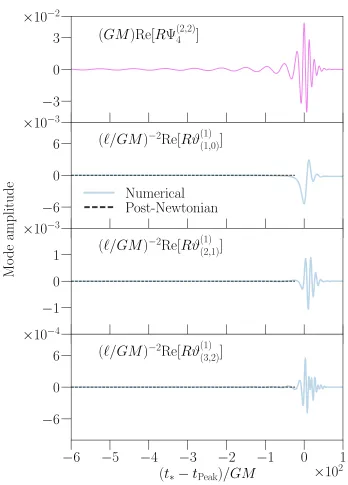
We find that the ringdown QNM spectrum is modified similarly to the head-on collision case (cf. Chapter5), while the inspiral is modified with a beating frequency

pattern, sourced by beating between the leading-order dCS scalar field and the GR

binary black hole background (cf. Fig.1.1).

Using numerical relativity to test the no-hair theorem

The final chapter of this thesis, Chapter7, considers another use-case for numerical

relativity in testing general relativity.

Recall from Sec.1.3 that one of the tests we can perform with gravitational wave

observations is a test of theno-hair theorem, which involves the ringdown portion of

the gravitational wave signal. One can also perform a test, (as in [14] for GW150914) to simply look for the least-damped quasi-normal mode in the ringdown portion of

the signal, and check that its parameters are consistent with those predicted by GR.

Ringdown, in this case, refers precisely to the regime where the gravitational wave

can be described as a set oflinear QNM perturbations on a stationary black hole

background. After merger, the spacetime around the resulting single black hole can

still potentially contain non-linearities – it takes some time after merger to settle

into the ringdown regime.

In order to perform a no-hair theorem or least-damped QNM test, we must thus choose a portion of the post-merger gravitational waveform that is truly within this

ringdown regime. If we start our test too early in the gravitational waveform, then

our analysis will contain systematic errors from trying to model something that

is non-linear as linear. In fact, the post-merger analysis for GW150914 [14] saw

(24)

the 90% credible region for the inferred QNM parameters didnotoverlap with that

predicted by GR and QNM perturbation theory. However, when the analysis window was shifted to a later time, where the ringdown description was more faithful, the

regions overlapped.

How should we choose the start time of ringdown? Past authors have used properties

of numerical relativity gravitational waveforms to estimate this regime [110,44,124,

33]. However, in a numerical relativity simulation, we have access not only to the

computed gravitational waveform, but alsothe whole spacetime itself (cf. Fig.1.2).

Thus, when asking ourselves questions about the amount of non-linearity present in the waveform, we can instead turn directly to the associated strong-field region in

the simulation.

In Chapter 7, we offer a numerical-relativity based approach to choosing the start

time of binary black hole ringdown. We use various algebraic and geometric

quantities put forth in [93, 187] that measure Kerrness, or closeness to a Kerr

spacetime on a given spatial slice. We present a formalism to associate the values of

the Kerrness measures to the amount of non-linearity present in the spacetime. We

see that as the post-merger numerical relativity simulation progresses, each spatial slice gets closer and closer to a linearly perturbed Kerr spacetime, with fewer and

fewer non-linearities. We derive a prescription for then mapping this information

onto the gravitational waveform from the simulation.

The result thus gives a gravitational waveform with a measure of the amount of

non-linearity (let’s call itε) at each time on the post-merger part of the waveform. This ε can thus act as a systematic error measure on a ringdown analysis, for it denotes precisely how much non-linearity is contaminating a linear analysis. We

produced such a result for the numerical relativity simulation of GW140915 used in the LIGO detection paper [11]. Our analysis found that the start times of ringdown

chosen in the testing GR companion paper [14] were too early, as the spacetime

still contained a fair amount of non-linearity. Subsequent, independent studies on

testing GR with binary black hole ringdowns explicitly confirmed our results [123,

65,57].

1.6 Looking forward

Our motivation for all of the projects presented in this thesis can be summarized

by the following: we know that at some length scale, general relativity must break

(25)

Closeness to linearly perturbed Kerr spacetime

Gravitational Wave

Time

BH

Strong-field Region

Figure 1.4: Schematic of the method of determining the start time of binary black hole ringdown, as discussed in Chapter 7. Time moves from the left to the right. The top figures show snapshots of the strong-field region around the final black hole (denoted BH) on three spatial time-slices. We show a Kerrness measure on the on slice, which in time settles to a value consistent with that of a linearly perturbed Kerr spacetime. How close the strong-field region is to the linear regime can then be mapped onto the gravitational waveform. This information on the gravitational waveform can then be used to inform the start time of ringdown, which requires being in a linear regime.

Merging binary black holes probe the strong-field, non-linear, dynamical regime of gravity, and gravitational waves from these systems could perhaps contain signatures

of such a theory.

Our goal of generating precise beyond-GR gravitational waveforms using numerical

relativity is to try to probe such signatures (or show their absence) using

model-dependent tests of general relativity. Similarly, our goal of using numerical relativity

to inform the start time of binary black hole ringdown is aimed to be able to precisely

probe beyond-GR signatures in the post-merger signal.

There is much work to be done. We need to generate more dCS waveforms in order

to perform a model-dependent test of GR with gravitational wave detector data.

We must generate enough waveforms to produce a dCS surrogate model for rapid

(26)

We also need our waveforms to be more accurate. Gravitational wave detectors

with higher singal-to-noise ratios (for some systems) than LIGO, such as the Laser Interferometer Space Antenna (LISA), will come online in this century [27, 22].

Numerical relativists need to make sure that general relativity and beyond-GR

waveforms are at the level of accuracy where numerical errors in the waveform are

lower than the level of noise on the detectors. This should be feasible with future

codes [114].

We need to consider other beyond-GR theories of gravity, in addition to dynamical

Chern-Simons theory. The techniques and code that we have generated and used in Chapters2, 3, 4, 5, and6can be used for Einstein-dilaton-Gauss-Bonnet gravity

(cf. Eq.1.4), and other higher-curvature effective field theories, by simply changing

the source term.

The past century has seen the triumph of general relativity, and perhaps the coming

(27)

C h a p t e r 2

NUMERICAL BINARY BLACK HOLE MERGERS IN

DYNAMICAL CHERN-SIMONS GRAVITY: SCALAR FIELD

[1] Maria Okounkova et al. “Numerical binary black hole mergers in dynamical Chern-Simons gravity: Scalar field”. In:Phys. Rev.D96.4 (2017), p. 044020. doi:10.1103/PhysRevD.96.044020. arXiv:1705.07924 [gr-qc].

Abstract

Testing general relativity in the non-linear, dynamical, strong-field regime of gravity

is one of the major goals of gravitational wave astrophysics. Performing precision

tests of general relativity (GR) requires numerical inspiral, merger, and ringdown

waveforms for binary black hole (BBH) systems in theories beyond GR. Currently,

GR and scalar-tensor gravity are the only theories amenable to numerical simula-tions. In this article, we present a well-posed perturbation scheme for numerically

integrating beyond-GR theories that have a continuous limit to GR. We demonstrate

this scheme by simulating BBH mergers in dynamical Chern-Simons gravity (dCS)

to linear order in the perturbation parameter. We present mode waveforms and

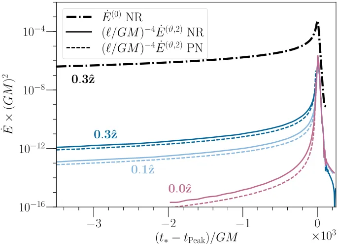
energy fluxes of the dCS pseudoscalar field from our numerical simulations. We

find good agreement with analytic predictions at early times, including the absence

of pseudoscalar dipole radiation. We discover new phenomenology only accessible

through numerics: a burst of dipole radiation during merger. We also quantify the

self-consistency of the perturbation scheme. Finally, we estimate bounds that GR-consistent LIGO detections could place on the new dCS length scale, approximately

` .O(10)km.

2.1 Introduction

General relativity has been observationally and experimentally tested for almost a

century, and has been found consistent with all precision tests to date [206]. But

no matter how well a theory has been tested, it may be invalidated at any time

when pushed to a new regime. Indeed, there are many theoretical reasons to believe

that general relativity (GR) cannot be the ultimate description of gravity, from

(28)

Moreover, from the empirical standpoint, all precision tests of GR to date have

been in the slow-motion, weak-curvature regime. With the Laser Interferometer Gravitational Wave Observatory (LIGO) now detecting the coalescence of compact

binary systems [10,5,16], we finally have direct access to the non-linear, dynamical,

strong-field regime of gravity. This is an arena where GR lacks precision tests, and

it may give clues to a theory beyond GR. The LIGO collaboration has already used

the detections of GW150914, GW151226, and GW170104 to perform some tests of

GR [14,16], but these are not yet very precise: a model-independent test gives 96%

agreement with GR.

Both black hole (BH) and neutron star (NS) binaries probe the strong-field regime. However, NSs have the added complication that the equation of state of dense

nuclear matter is presently unknown. Until more is known about the equation of

state, we must rely on binary black holes (BBHs) for precision tests of GR. Yunes,

Yagi, and Pretorius argued [216] that the lack of understanding of BBH merger

in beyond-GR theories severely limits the ability to constrain gravitational physics

using GW150914 and GW151226. Thus, to perform tests of GR with BBHs, we

require inspiral, merger, and ringdown waveform predictions for these systems,

which can only come from numerical simulations.

To date, BBH simulations have only been performed in GR and scalar-tensor grav-ity [43] (note that BBHs in massless scalar-tensor gravgrav-ity will be identical to GR,

under ordinary initial and boundary conditions). There are a huge number of

beyond-GR theories [43], and for the vast majority of them, there is no knowledge

of whether there is a well-posed initial value formulation, a necessity for

numer-ical simulations. Indeed, there is evidence that dynamnumer-ical Chern-Simons gravity,

the beyond-GR theory we use here as an example, lacks a well-posed initial value

formulation [74].

Our goal is to numerically integrate BBH inspiral, merger, and ringdown in theories

beyond GR that are viable but that do not necessarily have a well-posed initial value problem. This goal is relevant even for those only interested in parametric,

model-independent tests, because there is presently no theory guidance for late-inspiral and

merger waveforms in theories beyond GR.

We are only interested in theories that are sufficiently “close” to GR: for a theory to

be viable, it has to be able to pass all the tests that GR has passed. This motivates an

effective field-theory (EFT) approach. We assume that there is a high-energy theory

(29)

of GR with corrections does not need to capture arbitrarily short-distance physics.

Such a theory is valid up to some cutoff, and modes shorter than this distance scale are said to be outside of the regime of validity of the EFT. The EFT only needs to be

well-posed for the modes within the regime of validity. This can be accomplished

with perturbation theory.

We present a perturbation scheme for numerically integrating beyond-GR theories

that limit to GR. For such a theory, we perturb it about GR in powers of the small

coupling parameter. We collect equations of motion at each order in the coupling,

creating a tower of equations, with each level inheriting the same principal part

as the background GR system. The well-posedness of the initial value problem in GR [203] thus ensures the well-posedness of this framework, even if the “full”

underlying theory may not have a well-posed initial value formulation.

In this study, we apply our perturbation framework to BBH mergers in dynamical

Chern-Simons gravity (dCS) [18] to linear order in perturbation theory. This theory

involves a pseudoscalar field coupled to the parity-odd Pontryagin curvature invariant

with a small coupling parameter, and at linear order gives a scalar field evolving on

a GR BBH background.

There are a number of theoretical motivations for considering dynamical

Chern-Simons. The dCS interaction arises when cancelling gravitational anomalies in chiral theories in curved spacetime [72, 79, 21], including the famous

Green-Schwarz anomaly cancellation in string theory [95] when compactified to four

dimensions [18, 157, 158]. DCS also arises in loop quantum gravity when the

Barbero-Immirzi parameter is allowed to be a spacetime field [192, 134]. From

an EFT standpoint, dCS is the lowest-mass-dimension correction that has a

parity-odd interaction. All other EFTs at the same mass dimension have parity-even

interactions, so the phenomenology of dCS is distinct [212]. The dCS interaction

was also included in Weinberg’s EFT of inflation [204].

From a practical standpoint, there are already a large number of dCS results in

the literature that we can compare against [214, 212, 210, 209, 211, 117, 184],

including post-Newtonian (PN) calculations for the BBH inspiral. One of the more

important results is that scalar dipole radiation is highly suppressed in dCS during

the inspiral [212]. Dipole radiation is present in scalar-tensor theory and

Einstein-dilaton-Gauss-Bonnet (EdGB), and enters with two fewer powers of the orbital

velocity (i.e. 1 PN order earlier) than the leading quadrupole radiation of GR. This

(30)

the dipole is suppressed. As a result, the perturbative treatment of dCS will be valid

for a longer period of inspiral than scalar-tensor or EdGB.

The paper is organized as follows. Sec. 2.2 covers the analytical and numerical

formalisms. More specifically, in Sec.2.2 we introduce dynamical Chern-Simons,

and in Sec. 2.2 we present the perturbation scheme, which is valid for any theory

with a continuous limit to GR. We discuss the numerical scheme in Sec.2.2(some

numerical details are in the Appendix). We present the results of numerically

im-plementing this formalism in dCS on three different binary mergers in Sec. 2.3. Sec. 2.3 reviews some previously-known analytic phenomenology of the BBH

in-spiral problem in dCS. Sec.2.3presents the waveform results, and2.3presents the

energy fluxes, both including comparison to PN. In Sec.2.3 we use the numerical

results to assess the validity of the perturbation scheme. In Sec. 2.3 we use the

numerical results to estimate the detectability of dCS and the bounds that could be

placed by LIGO detections. We conclude and discuss in Sec.2.4, and lay out plans

for future work.

2.2 Formalism

Throughout this paper, we set c = 1 and_~ = 1 so that [M] = [L]−1. Since there will be more than one length scale, we explicitly include factors of the reduced Planck massm−_pl2=8πGand the “bare” gravitational lengthGM, though quantities in our code are non-dimensionalized withGM = 1. Latin letters in the middle of

alphabet{i,j,k,l,m,n}are (3-dimensional) spatial indices, while Latin letters in the beginning of the alphabet{a,b,c,d}refer to (4-dimensional) spacetime indices. We follow the sign conventions of [203], andgabrefers to the 4-dimensional spacetime

metric, with signature(−+ + +), and with∇its Levi-Civita connection.

Action and equations of motion

The method we present in this paper applies to a large number of beyond-GR theories

that have a continuous limit to GR, but for concreteness we focus on dCS. We start

with the four-dimensional action

I =

∫

d4x√−g[LEH+Lϑ+Lint+Lmat+. . .], (2.1) where the omitted terms (. . .) are above the cutoff of our EFT treatment. Here

g without indices is the determinant of the metric, LEH is the Einstein-Hilbert

(31)

betweenϑand curvature terms, and Lmatis the Lagrangian for ordinary matter. In this paper, we are considering a binary black hole (BBH) merger in dCS, so we ignoreLmat.

Explicitly, these action terms are given by

LEH = m_pl2

2 R, Lϑ= −

1 2(∂ϑ)

2_, _(2.2a)

Lint =−mpl 8 `

2_ϑ∗

RR. (2.2b)

Here the Ricci scalar of gab is R. With our unit system, [g] = [L]0, coordinates carry dimensions of length, [x] = [L]1, and note that the scalar field ϑ has been canonically normalized,[ϑ] = [L]−1. We have omitted any potentialV(ϑ), soϑis massless and long-ranged, as appropriate for a “gravitational” degree of freedom.

In the interaction LagrangianLint, the scalar fieldϑis coupled to the 4-dimensional

Pontryagin density (also known as the Chern-Pontryagin density)∗RR,

∗

RR≡∗RabcdRabcd = ₂1abe fRe fcdRabcd, (2.3) whereabcdis the fully antisymmetric Levi-Civita tensor.

The coupling strength of this interaction is governed by the new parameter ` with dimensions of length. This parameter takes on specific values if this EFT arises from the low-energy limit of certain string theories [95] or to cancel gravitational

anomalies [21, 157, 158]. However, here we simply take it as a “small” coupling

parameter. In the limit that ` → 0, we recover general relativity with a massless, minimally coupled scalar field.

The coupling parameter conventions vary throughout the literature. To enable

comparisons, we express the couplings of a number of works in terms of our conventions. To put Yagi et al. [212] into our conventions, use

κYSYT ₌ 1

2m

2

pl, α YSYT

4 = −

mpl`2

8 , β

YSYT ₌₁_. _(2.4)

To convert Alexander and Yunes [18] into our conventions,

κAY ₌ 1

2m

2

pl, α AY 4 = +

mpl`2

2 , β

AY ₌ ₁_. _(2.5)

To compare with McNees et al. [133], use

κMSY₌

m−_pl1, αMSY= +` 2

(32)

The conventions of Stein [184] agree with ours (except for an inconsequential sign

change in the definition of ∗RR, which is compensated for by an additional sign everywhere∗RRappears).

Below we will perform an expansion in powers of`2. To simplify matters, we insert a dimensionless formal order-counting parameterεthat will keep track of powers of

`2_{. Expanding in a dimensionless parameter ensures that field quantities at different}

orders have the same length dimension.

Specifically, we replace the action in Eq. (2.1) with

Iε = ∫

d4x√−g[LEH+ Lϑ+εLint+ Lmat+. . .], (2.7) a one-parameter family of actions parameterized by ε. Formally, we recover the action in Eq. (2.1) whenε= 1.

Varying the action Eq. (2.7) with respect to the scalar field, we have the sourced wave equation

ϑ= εm₈pl`2∗RR, (2.8)

where= ∇a∇ais the d’Alembertian operator. Varying with respect to the metric gives the corrected Einstein field equations,

m2_plGab+mplε`2Cab=T_abϑ +T_abmat, (2.9)

whereGabis the Einstein tensor ofgab, and the tensorCabincludes first and second

derivatives ofϑ, and second andthirdderivatives of the metric,

Cab≡ cde(a∇dRb)c∇eϑ+∗Rc(ab)d∇c∇dϑ. (2.10) Since we are focusing on BBH mergers,T_abmat = 0. The scalar field’s stress-energy

tensorT_abϑ is given by the expression for a canonical, massless Klein-Gordon field,

T_abϑ = ∇_aϑ∇_bϑ− 1

2gab∇cϑ∇ c_{ϑ .}

(2.11)

From here forward we will drop the superscriptϑ.

(33)

Perturbation scheme

BecauseCabin Eq. (2.9) contains third derivatives of the metric, the “full” system

of equations for dCS likely lacks a well-posed initial value formulation [74]. In the

language of particle physics, this is equivalent to the appearance of ghost modes

above a certain momentum scale [77].

From the EFT point of view, though, the ghost modes and ill-posedness are nothing

more than the breakdown of the regime of validity of the theory, which should be

valid for long wavelength modes in the decoupling limit ` → 0. To excise the ghost modes and arrive at a well-posed initial value formulation, we expand about

ε = 0, which is simply GR coupled to a massless minimally-coupled scalar field and certainly has a well-posed initial value problem [203]. As a result, all higher

orders inεwill inherit the well-posedness of the zeroth-order theory by inheriting the principal parts of the differential equations.

We begin this order-reduction scheme by expanding the metric and scalar field in

power series inε,1

gab =g (0) ab +

∞ Õ

k=1 εk

h(_abk), (2.12a)

ϑ=

∞ Õ

k=0

εk_ϑ(k)_.

(2.12b)

Note that sinceεis dimensionless, eachϑ(k) has the same units asϑ, and similarly forh_ab(k). This expansion is now inserted into the field equations, which are likewise

expanded in powers ofε, and we collect orders homogeneous inεk, as below. This results in a “tower” of systems of equations that must be solved at progressively

increasing orders inε. This scheme is quite general and should apply to any theory that has a continuous limit to GR.

Orderε0

Zeroth order comes from taking ε → 0, which simply gives the system of GR coupled to a massless, minimally coupled scalar field,

m2_plGab[g(0)]=T (0)

ab , (2.13a)

(0)ϑ(0) =0, (2.13b)

1_{Note that this is not a Taylor series, since there is no factor of 1}_/_k_{! in the} _k_{th term. These}

(34)

where Gab[g(0)] is the Einstein tensor of the background metric g(0), (0) is the associated d’Alembert operator, andT(0) is the stress-energy of ϑ(0). This system certainly has a well-posed initial value problem.

Because of the explicit presence of ε in front of Lint in the action [Eq. (2.7)], Cab does not appear in the metric equation (2.13a), and the Pontryagin source does not

appear on the right-hand side of the scalar equation (2.13b). These terms have been

pushed to one order higher and will appear below.

On general grounds, we expect that any initially non-vanishing scalar field will

radi-ate away within a few dynamical times. Similarly, if we start with aϑ(0) = 0 initial condition and impose purely outgoing boundary conditions, ϑ(0) will remain zero throughout the entire simulation. Therefore, rather than simulating a vanishingly

smallϑ(0), we simply analytically assume thatϑ(0) = 0.

Therefore, at orderO(ε0), the system will simply be

Gab[g(0)]= 0, (2.14)

and the solution will be

(g(0), ϑ(0))= (gGR,0), (2.15)

wheregGR_{is a GR solution to the BBH inspiral-merger-ringdown problem.}

Orderε1

Continuing to linear order inε, we find the system

m_pl2G(_ab1)[h(1);g(0)]= −mpl`2C_ab(0)+T_ab(1), (2.16a)

(0)ϑ(1)+(1)ϑ(0) = m8pl` 2_[∗

RR](0). (2.16b)

As noted above, the explicit presence ofεin the action (2.7) and equations of motion [(2.8) and (2.9)] lead toC(0)and[∗RR](0) appearing in theseε1equations strictly as source terms. By construction, the principal part of this differential system is the

same as the principal part of theO(ε0)system, and thus it inherits its well-posedness property. This is true at all higher orders in perturbation theory.

(35)

evaluated on the background quantities (g(0), ϑ(0)). Similarly, [∗RR](0) is the Pon-tryagin density evaluated on the background spacetime metricg(0). Finally,T_ab(1) is the first-order perturbation to the stress-energy tensor; sinceTab is quadratic in ϑ,

T_ab(1) has pieces both linear and quadratic in ϑ(0) (the quadratic-in-ϑ(0) pieces are linear inh(1)).

The crucial property at this order is that both C(0) andT(1) are built from pieces linear and quadratic in ϑ(0). At order O(ε0), we found that ϑ(0) = 0. Therefore, when evaluated on theO(ε0)solution [Eq. (2.15)], these both vanish,

C_ab(0)[ϑ(0) =0]=0, T_ab(1)[ϑ(0) = 0]=0. (2.17) Therefore, at order O(ε1) in perturbation theory, evaluating on the background solution, we have the system

m2_plG(_ab1)[h(1);g(0)]= 0, (2.18a)

(0)ϑ(1) = m₈pl`2[∗RR](0). (2.18b) In the metric perturbation equation (2.18a), starting withh(1) =0 initial conditions and imposing purely outgoing boundary conditions will enforceh(1) = 0 throughout the entire simulation. Similarly, we can argue that small perturbations ofh(1)would radiate away on a few dynamical times, since there is no potential to confine the

metric perturbations. Once again, rather than simulating a vanishingly small field,

we will just analytically assume thath(1) = 0. Therefore, at orderO(ε1), there is no metric deformation, and the system is only Eq. (2.18b), driven by the background

system (2.14) which generates the source term[∗RR](0).

Orderε2

This perturbation scheme can be extended to any order desired. Although this paper

reports only on work extending through O(ε1₎_{, we sketch the derivation of}_O(_ε2₎_,

since that is the lowest order where a metric deformation is sourced.

Schematically, the system at O(ε2), after accounting for the vanishing of ϑ(0) and

h(1), is

m_pl2G(_ab1)[h(2)]=−mpl`2C_ab(1)[ϑ(1)]+T_ab(2)[ϑ(1), ϑ(1)], (2.19a)

(0)ϑ(2) =0. (2.19b)

(36)

were quadratic inh(1)or built from the product of h(1)×ϑ(1). In (2.19b),`2[∗RR](1)

is proportional toh(1)and thus vanishes, as do terms such as(1)ϑ(1)(linear inh(1)) and(2)ϑ(0) (linear inϑ(0)).

We leave detailed discussion of orderO(ε2)to future work [144].

Summary and scaling

Let us briefly summarize the perturbative order-reduction scheme and discuss the

scaling of different orders. The system at ordersε0andε1is

O(ε0): Gab[g(0)]= 0, ϑ(0) =0, (2.20a)

O(ε1): (0)ϑ(1) = m₈pl`2[∗RR](0), h(1) =0, (2.20b) and if we were to continue toO(ε2),

O(ε2): G(_ab1)[h(2)]= m−_pl2T_abeff, ϑ(2) =0, (2.20c) whereT_abeff may be determined from the right hand side of Eq. (2.19a).

Zeroth order (2.20a) is just vacuum GR, which has no intrinsic scale. As is very

common in numerical relativity simulations, the coordinates used in the simulation

are dimensionless and in units of the total ADM mass, Xa = xa/(GM). This means that ∇ may be non-dimensionalized by pulling out a factor of (GM)−1, Riemann may be non-dimensionalized by pulling out a factor of(GM)−2, etc.

Meanwhile, the new length scale and coupling parameter` enters at first order. If we non-dimensionalize the derivative operator and curvature tensors in Eq. (2.20b),

we will find

(GM)−2(0)ϑ(1) = mpl

8 `

2₍

GM)−4[∗RR](0). (2.21) We therefore define the dimensionless scalar fieldΨvia

ϑ(1) ₌ mpl 8

`

GM

2

Ψ. (2.22)

ThenΨwill satisfy

(0)Ψ= [∗RR](0). (2.23)

Thus the analytic dependence ofϑ(1) on(`/GM)has been extracted. The solution

(37)

All of the results that we present will be given in terms of powers of the dimensionless

coupling(`/GM). We will also compare to known post-Newtonian results [211], that were presented in terms of αYSYT

4 . To perform the comparison, we use the

conversion given in Eq. (2.4).

Finally, though we do not address O(ε2) simulations in this paper, we should still study how h(2) scales with ` and (GM). Since the perturbative scheme preserves the units of length of fields,[h(k)]= [g]= [L]0is already dimensionless; however, it still depends on(`/GM) in a specific way. When we move to units in which we measure lengths and times in units of(GM), we find it is appropriate to define a scaled metric deformationΥvia

h(_ab2) ≡

`

GM

4

Υab. (2.24)

Then this dimensionless quantityΥwill satisfy an equation that is schematically

∇2Υ+L.O.T. ∼ (∇Ψ)2+(∇Ψ)(∇R)+(∇2Ψ)R, (2.25) where L.O.T. stands for lower order terms, and all derivatives and curvatures are

O(ε0)dimensionless quantities.

Numerical scheme

For the order ε1 part of the order reduction scheme, our overall goal is to solve Eq. (2.23) on a dynamical background metric. We co-evolve the metric and the

scalar field, where Eq. (2.23) is driven by Eq. (2.20a). The whole system is simulated

using the Spectral Einstein Code (SpEC) [198], which uses the generalized harmonic

formulation of general relativity in a first-order, constraint-damping system [121]

in order to ensure well-posedness and hence numerical stability. We have added

a scalar field module that is similarly a first-order, constraint-damping system,

following [105], as outlined in App.2.A.

The code uses pseudospectral methods on an adaptively-refined grid [128, 189],

and thus numerical convergence with resolution of both the metric variables and the

scalar field is exponential. We demonstrate the numerical convergence of the scalar

field in App.2.A.

The initial data for the binary black hole background is a superposition of two

Kerr-Schild black holes with a Gaussian roll-off of the conformal factor around each black

(38)

of approximate dCS solutions around isolated black holes, and is given in more

detail in Sec.2.3.

The metric equations are evolved in a damped harmonic gauge [190, 120], with

excision boundaries just inside the apparent horizons [104, 177], and

minimally-reflective, constraint-preserving boundary conditions on the outer boundary [172].

The scalar field system, meanwhile, uses purely outgoing boundary conditions

modi-fied to reduce the influx of constraint violations into the computational domain [105].

The Pontryagin density source term∗RRis computed throughout the simulation in a 3+1 split from the available spatial quantities as outlined in App.2.B.

2.3 Results

Background: Phenomenology of binary black hole inspirals in dCS

To give the proper context for our numerical results, we first review the

previously-known phenomenology relevant to this problem. Analytical and numerical results

are known for isolated black holes in the decoupling limit, and analytical results are known for the binary black hole problem in the decoupling limit and at slow

velocities (v/c 1).

Any spherically-symmetric metric will have vanishing Pontryagin density.2 Thus the Schwarzschild solution with vanishing scalar field is already a solution to the

“full” dCS system. An isolated spinning black hole in dCS, however, is not given

by the Kerr solution of GR [61, 214,116, 210]; the scalar field is sourced, and the

metric acquires corrections. Analytical results for the leading-order, small-coupling corrections to the Kerr metric have been found in the slow-rotation approximation

(a M) [214,116,210,131]. Additionally, numerical results have been found for the scalar field for general rotation [117,183]. The leading-order correction to Kerr

is dipolar scalar hair, while the scalar monopole vanishes. This vanishing scalar

monopole means that scalar dipole radiation is heavily suppressed in dCS. At a large

radius away from an isolated black hole labeled by A, the dipolar scalar field goes

2_{This is straightforward to verify with a computer algebra system, using the canonical form for}

a spherically symmetric metric, ds2 = −e2α(t,r)dt2+e2β(t,r)dr2+r2dΩ2. Since it is true in this coordinate system, it is true in general. This is also proven in App. A of [97] following a tensorial approach. Finally, one can appeal to a symmetry argument. If the metric is invariant under an

O(3)isometry, then the curvature tensor and∗_RR_{, being tensorial objects built only from}_g_{, must}

also be i