ABSTRACT
AKHAVAN-TABATABAEI, RAHA. A Markov Chain Framework for Approximation of Cycle Time in Semiconductor Manufacturing Toolsets. (Under the direction of Dr. Yahya Fathi.)
Accurate and e¢ cient cycle time approximation is a critical issue in semiconductor manufacturing systems (SMS), since it facilitates the subsequent production planning and scheduling activities and helps reduce the overall cycle time. Presently computer simulation is a common approach to cycle time approximation and performance analysis in SMS. Simulation models however, have several inherent short-comings, and it can be di¢ cult and time-consuming to use such models to explore various what-if questions. Compared with simulation models, analytical approaches based on queuing theory can be much faster in achieving reasonable results, and they typically provide more insights for performance improvement. But in the context of the SMS, performance of the queuing models has not been satisfactory due to inaccurate results.
We believe that a major cause of this poor performance is the application of operational rules in SMS. These rules are typically invented by line managers so as to interfere with various components of the system such as the arrival process, the service process, and the repair process, in an attempt to increase the speed of the production ‡ow. Deployment of such rules, however, creates dependen-cies among these components of the system which are typically not captured by classical queuing models. This, in turn, could render the results obtained via these models somewhat inaccurate and unsatisfactory.
In this dissertation we propose a Markov chain framework to model the behavior of a toolset (workstation) in SMS under various operational rules, and employ this model to approximate, with a relatively high degree of accuracy, the long-run average cycle-time of jobs at the toolset.
We then use these steady state probabilities to calculate the expected value of WIP for the system, and employ Little’s law to determine the long-run average cycle time for the workstation.
Subsequently we extend this Markov chain model to develop a framework for modeling toolsets with other underlying conditions and assumptions. The scenarios that we consider include toolsets with non-exponential distributions for the arrival and the service processes, toolsets with heteroge-neous servers, and servers that are prone to multiple types of failure.
In order to evaluate the accuracy of this approach, we conduct a comprehensive computational experiment in which we compare the numeric values obtained via the resulting Markov models with those obtained via the corresponding simulation models. The results of this experiment show that our proposed approach obtains numeric values that are signi…cantly more accurate than those obtained via classical queuing models.
A Markov Chain Framework for Approximation of Cycle Time in Semiconductor
Manufacturing Toolsets
by
Raha Akhavan-Tabatabaei
A dissertation submitted to the Graduate Faculty of
North Carolina State University
in partial fulfillment of the
requirements for the Degree of
Doctor of Philosophy
Industrial Engineering
Raleigh, North Carolina
2011
APPROVED BY:
Dr. Tom Culbreth
Dr. Yahya Fathi
Chair of Advisory Committee
Dr. George Shanthikumar
Dr. Reha Uzsoy
BIOGRAPHY
ACKNOWLEDGEMENTS
I want to express my deepest gratitude to my adviser Dr. Yahya Fathi for his utmost support, patience and understanding during the course of preparing this dissertation. The persuasion and encouragement that I have received from him have constantly energized my work and due to his attention and care I never felt being far away from campus, although I actually was.
I would also like to thank Dr. George Shanthikumar who raised my interest in stochastic model-ing, introduced me to the topic of this dissertation and kindly accepted to serve on my committee. I truly appreciate the creative ideas and constructive comments that I have received from Dr. Reha Uzsoy throughout the course of my research. I sincerely thank Dr. Jim Wilson for the constant encouragement and advice and Dr. Tom Culbreth for providing me the opportunity of my …rst teaching experience at the university level and also serving on my committee. I also appreciate the time and e¤orts of Dr. Janice Wells to serve as the Graduate School representative on my committee. Additionally, I want to thank my colleagues at Universidad de los Andes for the invaluable opportunity that they have provided me and the continuous support and interest that they have shown towards my research. Speci…cally, I would like to thank Dr. Roberto Zarama and Dr. Andres Medaglia for their warm support.
TABLE OF CONTENTS
List of Tables . . . v
List of Figures . . . vi
1 Introduction . . . 1
1.1 Motivation and Problem Statement . . . 1
1.2 Research Objectives and Methodology . . . 2
1.3 Structure of Dissertation . . . 3
2 Background . . . 4
2.1 Overview of Semiconductor Manufacturing . . . 4
2.2 Literature Review . . . 10
2.3 Chapter Summary and Conclusions . . . 20
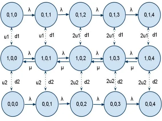
3 A State Dependent Markov Chain Model . . . 22
3.1 De…nitions and Notation . . . 22
3.2 The Basic State-Dependent Markov Chain Model . . . 23
3.3 Cycle Time Approximation Using The Proposed Model . . . 25
3.4 A Simulation Model for Generic Toolsets . . . 26
3.5 Chapter Summary and Conclusions . . . 27
4 Approximating Non-exponential Distributions . . . 28
4.1 Fitting Erlang Distributions . . . 28
4.2 Fitting Hyper-Erlang Distributions . . . 32
4.3 Solving The Steady State Equations Using QBD . . . 34
4.4 Chapter Summary and Conclusions . . . 38
5 Extension To More Complex Toolsets . . . 39
5.1 Toolsets with Heterogeneous Tools . . . 39
5.2 Toolsets with Multiple Failure Types. . . .40
5.3 Chapter Summary and Conclusions . . . 42
6 Numerical Results . . . 43
6.1 A Method for Performance Evaluation . . . 43
6.2 Case 1 - Toolset with Erlang Underlying Distributions . . . 44
6.3 Case 2 - Toolset with Hyper-Erlang Underlying Distributions . . . 47
6.4 Case 3 - Toolset with Lognormal Underlying Distributions . . . 48
6.5 Case 4 - Toolset with Gamma Underlying Distributions . . . 50
6.6 Case 5 - Toolset with Two Heterogeneous Tools . . . 52
6.7 Case 6 - Toolset with Two Failure Types . . . 53
6.8 Comparison with G/G/m Approximations . . . 54
6.9 Computational Requirements . . . 57
7 Concluding Remarks . . . 59
7.1 Summary of Completed Work . . . 59
7.2 Directions for Future Research . . . 61
References . . . 62
LIST OF TABLES
Table 6.2.1 Parameters ofa(t)and b(t)for Case 1 . . . 45
Table 6.2.2 Operational Rule Parameters . . . 45
Table 6.2.3 Eavg with Erlang Distributions . . . 46
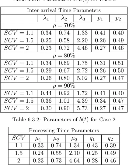
Table 6.3.1 Parameters ofa(t)for Case 2 . . . 47
Table 6.3.2 Parameters ofb(t)for Case 2 . . . 47
Table 6.3.3 Eavg with Hyper-Erlang Distributions . . . 48
Table 6.4.1 Parameters of the Lognormala(t)andb(t). . . 48
Table 6.4.2 Eavg with Lognormal Distributions and Exponential Fit . . . 49
Table 6.4.3 Eavg with Lognormal Distributions and Erlang Fit . . . 49
Table 6.5.1 Parameters of the Gammaa(t)andb(t). . . 50
Table 6.5.2 Eavg with Gamma Distributions and Exponential Fit . . . 51
Table 6.5.3 Eavg with Gamma Distributions and Hyper-Erlang Fit . . . 51
Table 6.6.1 Parameters ofa(t); b1(t)andb2(t)for Case 5 . . . 52
Table 6.6.2 Eavg for Heterogeneous Toolset Similar to Case 1 . . . 53
Table 6.7.1 Eavg for Toolset with Two Failure Types . . . 54
Table 6.8.1 Comparison withG=G=mApproximations - Case 1 . . . 55
Table 6.8.2 Comparison withG=G=mApproximations - Case 2 . . . 55
Table 6.8.3 Comparison withG=G=mApproximations - Case 3 . . . 55
Table 6.8.4 Comparison withG=G=mApproximations - Case 4 . . . 56
Table 6.8.5 Comparison withG=G=mApproximations - Case 5 . . . 57
Table 6.8.6 Comparison withG=G=mApproximations - Case 6 . . . 57
Table 6.9.1 Computational Requirements of Case 1 . . . 58
LIST OF FIGURES
Background
Figure 1. Major Steps of Processing A Single Layer of Oxide . . . 8
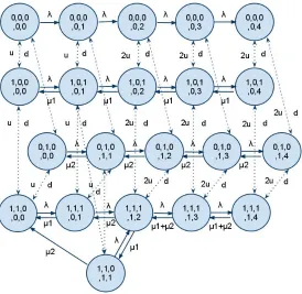
A State-Dependent Markov Chain Model Figure 2. Partial Rate Diagram of The Proposed Model . . . 24
Figure 3. Rate Diagram of Example 1 . . . 25
Approximating Non-exponential Distributions Figure 4. Example of A Two Phase Erlang Distribution . . . 29
Figure 5. Di¤erent Shapes of Erlang Distribution . . . 30
Figure 6. Lognormal Distribution Fitted by Erlang and Exponential . . . 31
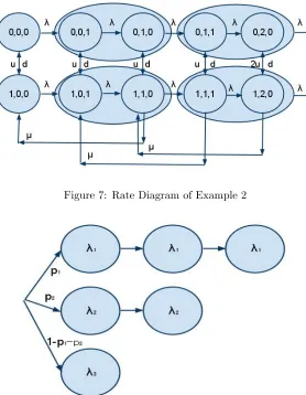
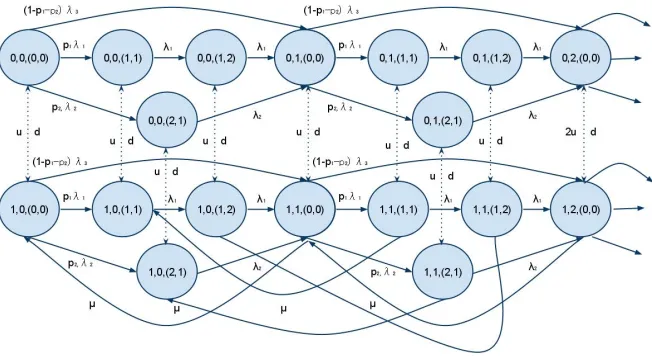
Figure 7. Rate Diagram of Example 2 . . . 32
Figure 8. The Three-Branch Hyper-Erlang Distribution . . . 32
Figure 9. Gamma Fitted by Exponential and Hyper-Erlang . . . 33
Figure 10. Rate Diagram of Example 3 . . . 35
Figure 11. Rate Diagram of Example 2 with No Breakdown . . . 36
Extension To More Complex Toolsets Figure 12. Rate Diagram of Toolset with Two Heterogeneous Tools . . . 41
Figure 13. Rate Diagram of Toolset with Two Failure Types . . . 42
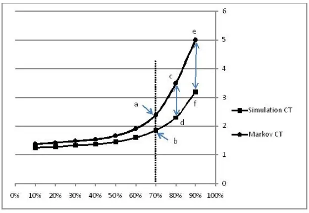
Numerical Results Figure 14. Calculation of Relative Error . . . 44
Figure 15. Utilization Graph for One Instance in Table 6.2.3 . . . 46
Figure 16. Utilization Graph for One Instance in Table 6.4.3 . . . 50
Figure 17. Utilization Graph for One Instance in Table 6.5.3 . . . 52
Figure 18. Utilization Graph for One Instance in Table 6.6.2 . . . 53
Figure 19. Utilization Graph for One Instance in Table 6.8.3 . . . 56
Appendix IV Figure 20. Utilization Graph 1 . . . 74
Figure 21. Utilization Graph 2 . . . 74
Figure 22. Utilization Graph 3 . . . 75
Figure 23. Utilization Graph 4 . . . 75
Figure 24. Utilization Graph 5 . . . 76
Figure 25. Utilization Graph 6 . . . 76
Figure 26. Utilization Graph 7 . . . 77
1
Introduction
1.1
Motivation and Problem Statement
Accurate and e¢ cient Cycle Time (CT) approximation has become an increasingly critical issue in semiconductor manufacturing (SM) industry over the past few years. This can be attributed to several factors including the constantly decreasing price of semiconductor products and rising competition among manufacturers. The faster a manufacturer can deliver its products to the market, the more expensive they can be sold and the more satis…ed become the customers of timely delivery. The prices of direct and indirect semiconductor products including central processing units, memory chips, digital cameras and cell phones decline very quickly. Leachman et al. [1] show by data that prices decline exponentially at fairly constant rates over the …rst two-thirds of product life, and then sometimes decline more slowly during the last third. The semiconductor industry faces fast and stable rates of price decline, whereby any delay on production output leads to lowered average selling prices for that output [2].
Speed of manufacturing is a very important performance metric for semiconductor fabrication fa-cilities (fabs). Semiconductor fabs are among the most capital-intensive and complex manufacturing plants in use today. Similar equipment and processes are applied to produce a variety of products including microprocessors, memories, digital signal processors and application-speci…c logic. Gener-ally, a small number of companies compete on selling interchangeable products or providing foundry services with similar process technologies to customers worldwide. Operational e¢ ciency is a crit-ical competitive advantage and relies on maximizing the outputs from the various input resources including a large …xed capital investment.
Due to these factors manufacturers are constantly under pressure to reduce cycle time and im-prove delivery performance. Accurate prediction of cycle time can greatly help production planning and scheduling of fabs. It is also well known that fab capacity and fab cycle time exhibit essentially an inverse relationship. Proper capacity prediction for a given cycle time is the key to a successful fab design. Such demands raise the question of how to quickly and accurately predict cycle time. However, this question is not easy to answer due to complicated tool speci…cations and process ‡ows in a semiconductor manufacturing system (SMS).
Shanthikumar et al. [3] consider simulation to be a common approach to cycle time approx-imation and performance analysis of SMS. At least in theory, simulation models can be adjusted precisely to meet various experimental purposes. They can be useful in verifying the assumptions and propositions of capacity planning and scheduling models. However, a simulation model has inherent shortcomings. It requires an enormous amount of input data, including equipment details, Work-In-Progress (WIP), management policies, and product information to produce reasonably ac-curate results. It also requires substantial resources to maintain and update. Based on the nature of simulation modeling, multiple replications are needed to perform proper statistical analysis. There-fore, it can be di¢ cult and extremely time-consuming to explore what-if questions. Compared with simulation, analytical approaches based on Little’s law and queueing theory can be much faster in achieving reasonable results and providing more insight for performance improvement [3].
Queueing theory is a powerful tool to evaluate the performance of a manufacturing system and can play an important role in assessing the performance of a semiconductor manufacturing line. This theory gives us insight into the trade-o¤ between cycle times and throughput rates. Possibly because of its simplicity and qualitative insight, theM=M=1queue, as well as its variations such as G=G=1,G=G=mand others, are widely used in this …eld.
been unsatisfactory due to their lack of accuracy [3].
Usually fabs are constructed as job-shop systems where, similar pieces of manufacturing equip-ment, known astools, are grouped together intotoolsets to perform similar processes. Batches of products-to-be, known as lots, move between these toolsets according to the recipe of that product to be processed through various steps or operations.
Several factors contribute to the inaccuracy of classical queueing theory when applied to SMS toolsets. Among others, multiple products and operations on one toolset, batching and set up requirements, re-entrant processes, scrap and rework, lot split and merge and high variation in machine availability due to tool breakdown have been investigated in the literature.
We believe that one of the major contributors to the inaccuracy of classical queueing models is the violation of basic assumptions in these models. Classical queueing models assume that the sequence of inter-arrival times and the sequence of service times are mutually independent and each sequence consists of independent and identically distributed random variables.
Inter-arrival time in the context of SMS is de…ned as the time between the arrivals of consecutive lots to a toolset. Service time is de…ned as the time between the start and the completion of processing a lot at the toolset. This time includes the pure processing time, the time that the lot is actually being processed on the tool, as well as any interruptions due to tool failure or other causes and it also depends on the number of functional tools in the toolset.
The assumption of independence for inter-arrival and service times is frequently violated in SMS due to the fact that line managers intervene in the random processes of arrival and service in order to make the line ‡ow faster. For example they sometimes increase or decrease the arrival rate at a certain toolset based on the current queue size, by controlling the operations at another toolset upstream. Other examples include allocating more or less resources to repair failed tools based on how critical the toolset is to the overall output of the factory at a given time, or postponing the preventive maintenance (PM) due to high tra¢ c at a toolset. We refer to such informal interventions asoperational rules throughout this document.
1.2
Research Objectives and Methodology
The purpose of this research is to provide a queueing model to approximate the cycle time of toolsets in SMS. In the context of SMS toolset is referred to a workstation where a number of tools or machines are grouped together. All the tools of a toolset can perform the same tasks or operations on the products and work as parallel servers. A typical SMS fab consists of a collection of toolsets that are linked together through the process ‡ow of the products.
Our goal in this research is to accurately predict the long-run average time that a lot spends at a particular toolset to be processed for one of the operations in its process ‡ow, given the speci…c parameters of the toolset including the number of tools, the arrival and service processes and the operational rule applied. We expect this model to be able to quickly and accurately evaluate the impact of operational rules on the toolset cycle time and be an e¤ective aid to evaluate and analyze di¤erent what-if scenarios with a quick turnaround.
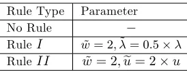
production. Throughout this research we consider two distinct types of such rules: Rule I that adjusts the mean inter-arrival time of lots andRule II that adjusts the mean time to repair a tool. We assume that both rules depend on the WIP level.
We develop a Markov chain model to approximate the cycle time of a toolset in both the presence and absence of operational rules. The state space of this model includes the current number of active tools as well as the WIP level in the system. The transition rates between the states of this model are determined based on the operational rule adopted for the toolset. Given the transition rates we solve the balance equations of the Markov chain to calculate the steady state probabilities. We then use the steady state probabilities to calculate the expected value of WIP for the system. Finally using Little’s formula we …nd the long-run average of cycle time for the toolset.
To verify the performance of this Markov chain model in cycle time approximation we build a simulation model to mimic the behavior of a typical toolset in a real SMS environment. We compare the cycle time approximation by the Markov chain model with the outcome of the simulation model as a measure of accuracy for the proposed model.
Based on the proposed Markov chain model for a basic toolset with operational rules we also present a framework to model toolsets with non-exponential distributions of arrival and service processes, toolsets with heterogeneous tools and toolsets with multiple types of failure. This general framework can be used to compare the impact of di¤erent line management policies, operational rules and what-if scenarios on the cycle time of SMS toolsets. It can also be employed for mid-to-long range capacity planning of the toolsets as well as assessing the fab cycle time using queueing networks analysis.
1.3
Structure of Dissertation
A brief overview of semiconductor manufacturing processes is presented in Chapter 2 followed by a survey of the relevant literature. The focus of this survey is mainly on the review of existing models for single-stage systems and queueing networks, proposed for manufacturing and semiconductor manufacturing systems. The shortcomings of these classical models in cycle time approximation of SMS toolsets are also brie‡y discussed.
In Chapter 3 we propose our approach to modeling the basic toolsets in SMS using a Markov chain model in order to improve the accuracy of cycle time approximation while maintaining fast response. The proposed model is capable of re‡ecting the e¤ects of operational rules on cycle time as well. We also discuss the development of a simulation model to examine the accuracy of predictions. Throughout the research the cycle time predictions of the proposed model are compared to the cycle time obtained by simulation for various scenarios.
The proposed Markov chain model in Chapter 3 assumes that all the underlying distributions of the arrival and service processes for the toolset are exponential. This assumption can be limiting in real SMS toolsets. To remove this potential limitation in Chapter 4 we expand the basic Markov chain model to include toolsets with non-exponential underlying distributions. We also present a method based on Quasi Birth-Death Processes in order to solve the steady-state equations of the extended Markov chain model for complex toolsets.
In Chapter 5 we extend the proposed Markov chain model of Chapter 3 to accommodate more complex situations in SMS, speci…cally toolsets with heterogeneous tools and toolsets with multiple failure types.
models. At the end of this chapter we study the computational e¢ ciency of the proposed framework for cycle time approximation and compare its computational requirements with simulation.
2
Background
2.1
Overview of Semiconductor Manufacturing
An integrated circuit commonly referred to as an IC or a semiconductor chip, is a complex device that consists of miniaturized electronic components and their interconnections. The production of IC’s is accomplished in a four-stage process that begins with raw plates of silicon or, less commonly, gallium arsenide that are called raw wafers. Wafers are grouped in lots, which travel together in a standard container and are destined for conversion to the same …nal product. The maximum lot size is usually between 20 and 100 wafers and di¤ers from one production facility to another. It may even di¤er from one product to another within the same facility. The most commonly seen lot size is a set of 25 wafers.
The …rst stage of IC production is called wafer processing or wafer fabrication. It is conducted in a clean room, where special means are employed to maintain low density of airborne particles. The termwafer fabis commonly used to mean a clean room in which wafer fabrication is conducted. Here the intricate miniature circuits for a number of identical chips are created on each wafer. The individual chips-to-be are referred to as dice. The circuitry is created by a lengthy and complex process, and the number of dice per wafer may vary from just a few to many hundreds.
This number depends on di¤erent factors including the diameter of the raw wafers, device geome-tries and quality yield. The latest achievement in high volume device geomegeome-tries is reported as 45nm, which indicates the width of an individual transistor on the device. Companies constantly improve wafer size and device geometry because of overall cost savings as a result of the larger number of dice per wafer. In this way by conducting the same number of process steps they can produce more dice. Wafer fabrication requires a long sequence of processing steps and involves many separate pieces of equipment, through which lots of wafers are routed in the traditional job shop fashion.
In the second stage of IC production commonly referred to aswafer probe,the individual dice on a wafer are tested for functionality by delicate electrical probes. Dice that fail to meet speci…cations are marked with an ink dot. Then the wafers are scored and broken into separate individual dice and the defective dice are discarded. In the third stage of production, called assembly, electrical leads are connected to the individual dice, which are then encapsulated in plastic or ceramic shells called packages. In the fourth stage of production, packaged chips are subjected to a …nal functional test and burn-in.
Perhaps the greatest single determinant of economic success for an IC manufacturer is the total process yield, de…ned as the fraction of individual dice that survives all stages of production and testing to emerge as salable packaged chips. Total yield may be 80% or higher for relatively simple circuits produced with mature technologies, but …gures below 10% are not uncommon for large, highly integrated products in the early stages of production [3].
The wafer fabrication stage dominates the economics of IC production, and it is here that semi-conductor manufacturers concentrate their research and development e¤orts. Wafer fabrication requires an enormous investment in plant and equipment. Because capital costs are high and vari-able processing costs are relatively low, high utilization of wafer fabrication equipment is a generally accepted goal in the semiconductor industry. Most competitive wafer fabs are operated on a two shift (day and night) basis for 7 days per week, but the amount of time spent actually processing wafers is limited by several factors such as preventive maintenance, setup, absence of quali…ed operators, end of shift e¤ects, and frequent episodes of unscheduled downtime.
A piece of equipment isidleif it is available for processing but is starved for work. Equivalently, the equipment is idle if it is neither processing wafers nor rendered unavailable for one of the reasons named above. The idleness rate for a piece of equipment is de…ned as the overall fraction of working hours that it spends in the idle condition. The conventional wisdom among semiconductor manufacturers is that the idleness rate for critical fabrication equipment should be no larger than 10%. Thus it will come as no surprise that wafers spend most of their time waiting in queues rather than being processed.
To set terminology, we de…ne the fab cycle time for a lot as the total number of working hours that elapse between its entry into the clean room and its exit. This same quantity will occasionally be called the manufacturing cycle time or manufacturing interval for wafer fabrication. The toolset cycle time is de…ned as the total working hours that elapse between the entry of a lot into the queue of a particular toolset and its exit after being processed by that toolset.
To better understand the magnitude of the queueing e¤ects in IC manufacturing, consider a wafer fab dedicated to production of a single, reasonably complicated product such as a laptop processor. Production of these processors involves a total of perhaps 600 distinct fabrication steps or operations. If we add the total times required to complete all these steps, assuming tools and people are always available for production, the total time might come to about one week. However, realistically it would typically take between 5 to 10 weeks to fabricate the same product. In the semiconductor industry it is common to describe this state of a¤airs by saying that the actual-to-theoretical ratio is between 5 and 10, or that the manufacturing cycle time is 5 to 10 times the theoretical.
This is widely recognized as a major problem for semiconductor manufacturers. In the case of customized products, the nature of the problem is obvious, since the order lead-time imposed on customers must be at least as large as the total manufacturing cycle time. On the other hand, standardized products can be made to stock, but here again, long manufacturing cycle times cause trouble because production must be based on forecasts of market demand for many months in the future, and major demand shifts are commonplace.
Moreover, product life cycles are short in the semiconductor industry, so the risk of obsolescence for …nished goods inventory is always present. Finally, research shows potential negative correlation between manufacturing cycle time and yield in wafer fabrication, which provides another strong motivation for reduction of throughput times.
Thus, it is essential that the designer of a wafer fabrication line has a means to predict key performance measures including average cycle time, given only the system characteristics that are known or can reasonably be approximated before the system goes into operation.
There exist two classes of wafer fabrication facilities in the industry. Research and Development (R&D) fabs, are dedicated to development of new products and processes and are usually a smaller version of a High Volume Manufacturing (HVM) fab. HVM fabs are designed for production of salable chips but the equipment, operating procedures and process ‡ows are essentially the same as an equivalent R&D fab but in a larger scale.
In this research, we mainly focus on the manufacturing cycle time of toolsets in HVM factories since the queueing systems formed in those fabs are far more complicated than in an R&D fab due to increased number of tools within each toolset as well as higher volume of lots ‡owing through the fab. E¤ective queuing models for HVM fabs can be easily modi…ed for an R&D fab too. In the following sections we will explain in more details the process of wafer fabrication in an HVM fab along with a brief introduction to major fabrication equipment, processing steps and ‡ow of the lots throughout the fab.
2.1.1 Wafer Processing
multiple operations are performed, plus ancillary equipment or facilities involved in closely related operations. Operators process lots on the inside of the U, and most equipment is positioned so that maintenance can be performed on the outside of the U. This area is called a chase, which is usually outside of the clean room. Companies have recently come up with newer layout plans such as a ballroom setting in which there are no bay/chase divisions and all pieces of equipment are put next to each other in a very large ballroom shaped space.
Each lot entering the clean room has an associated process ‡ow, often called a recipe, which consists of precisely speci…ed operations executed in a prescribed sequence on designated toolsets. If all goes well, this exact sequence of operations is performed, but sometimes inspections reveal that an operation was not executed to speci…cation, in which case, some or all of the wafers in the lot are either scrapped or reworked.
Integrated circuit fabrication involves the creation of multiple layers on a silicon plate, hence using the term wafer to refer to the silicon plates. The operations involved in the creation of each successive layer are essentially the same, so lots can, and typically do, return repeatedly to the same toolsets for completion of the subsequent layers.
2.1.2 Equipment Categories and Major Process Steps
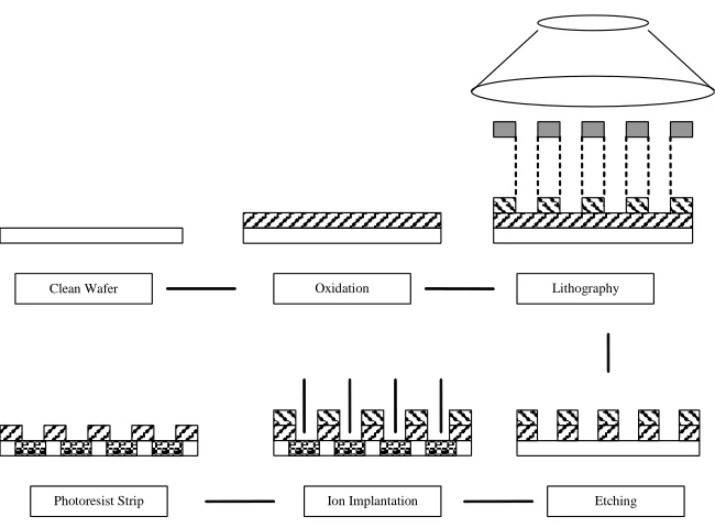
As noted before, each piece of equipment can perform one or multiple operations on the wafers. On the other hand, a fab can possess multiple pieces of the same equipment, commonly referred to as tools. The term toolset refers to a set of similar tools that are capable of performing the same operations and are grouped together in a single workstation. These toolsets usually perform one of the …ve major categories of operations involved in creating the successive layers on the silicon wafers. Figure 1 shows a simpli…ed graph of these steps and changes that they make on the wafer. A brief description of each category of operations follows and more details are given in [29] and [6].
1. Oxidation -A thin layer of material is deposited on the surface of the wafer to form a layer of the integrated circuit. The wafers must be cleaned within a speci…ed time before the operation is performed, to avoid particle contamination. Di¤erent oxide deposition technologies include chemical vapor deposition, spin on glass and physical vapor deposition (sputtering).
Clean Wafer Oxidation Lithography
Etching Ion Implantation
Photoresist Strip
3. Etching - Circuits are de…ned by etching away the portion of the oxide layer that is not protected by photoresist. There are two etching technologies used in the fabs; wet etching and plasma etching, also known as dry etching. The latter (more precise) technology is more heavily used, but wet etching is more complicated and needs more attention because of the possible inaccuracies that can happen.
4. Ion Implantation -In order to change the electrical properties of the surface not protected by the photoresist, the wafer is exposed to accelerated ions which are implanted to a predetermined depth and concentration. Boron, phosphorus, and arsenic ions are most frequently implanted because even a small number of their ions will dramatically alter the electrical properties of the underlying silicon.
5. Photoresist Strip -Finally, the pattern of photoresist that remains on the wafer after litho-graphy is removed (stripped) using a process similar to etching. Equipment which carry out this operation are commonly referred to as planar tools.
In addition to these …ve types of operations, many cleaning, measurement and inspection opera-tions are performed throughout the fab. The cleaning operaopera-tions prevent contamination of the wafer, and the inspection and measurement operations are performed to identify defective wafers, which are then scrapped or reworked. Di¤erent kinds of integrated circuits require di¤erent processing steps during fabrication, and thus, have di¤erent process ‡ows through the fab. Production facilities (as opposed to R&D labs) usually make more than one type of product. The processing technology changes quite frequently as well and therefore there is substantial diversity in product routing when the operations of any given fab are examined over a period of several years.
As stated earlier, an individual lot of wafers may visit one or more pieces of equipment repeatedly during the course of its fabrication. This phenomenon is referred to as re-entrant ‡ow. In particular, it is often necessary to use the same photo-lithography machine (stepper or aligner) in the creation of each layer. Ion implanters and inspection stations may also be visited repeatedly. Deposition equipment and plasma etchers are often dedicated to a single operation in a single process; it is therefore common for them to be visited only once during the entire fabrication sequence.
2.1.3 Flow Control in HVM Fabs
Most HVM fabs are designed as classic job shop operations, in which lots with diverse characters are routed through a collection of general purpose work centers for execution of prescribed operations. The performance of a job shop is a¤ected by the ‡ow control mechanisms employed, including the input control, routing and sequencing rules built into the shop’s operating system. Some of these routing and sequencing rules include lot-to-lens dedication for lithography operations and ion-implant run rules that are described here brie‡y.
Lot-to-lens dedication states that if the lithography process is done on a particular lot by a certain tool that lot has to go through the exact same tool for its subsequent lithography operations on higher layers. The reason is that lenses which are used in lithography to focus ultraviolet light on the mask, and subsequently onto the wafer through the patterns on the mask, cannot be built quite identically in a microscopic scale. The di¤erence, although minute, can cause misalignment between successive layers. Therefore, when processing the critical layers on a wafer, each lot has to go through the exact same piece of equipment that has laid the …rst layer onto the wafers in that lot.
reached, the recipe should be changed on the tool and lots with a di¤erent implant ion should be started on that machine.
Another factor that causes the ‡ow of lots through the fab to be stochastic is the processing of monitor lots or engineering lots. Due to high quality standards in most semiconductor companies, after any maintenance of the tools or any modi…cation in recipe a number of monitor lots or engineer-ing lots are run through the tool and possibly the tools that conduct subsequent operations. These lots are not considered as production lots and will be scrapped eventually. Their role is to make sure that the tools are quali…ed to manufacture within the required speci…cations after maintenance or recipe change.
Also for operations that require high accuracy such as lithography, after processing a number of lots one look-ahead (or send-ahead) lot is processed and tested before the rest of the lots in the queue are processed on that tool. This action is taken to make sure that the tool is still maintaining its quali…cations to process the lots.
Hot lots are another category of productions lots. These are lots with higher priority than any other lot waiting in the queue. Their priority may be caused by many di¤erent reasons, including split lots that are going to be merged with the mother lot in a few steps from the existing operation. This type of lots is especially common in R&D fabs where many experiments are performed on the process.
Processing of lots in a queue at a certain toolset is not always done on a First-In-First-Out (FIFO) basis. However, within a queue of lots from the same product type and same operation FIFO is conducted as the general policy.
2.1.4 Implicit Operational Rules
The operational rules are integrated with the operation of the SMS toolsets. These rules are often implicit and unwritten, decided and implemented by the line managers and operation managers based on their observation of the factory ‡ow and their knowledge of the situation at the upstream and downstream toolsets. These rules can be divided into two categories ofarrival-control rules and
PM-control rules.
The arrival-control or dispatching rules refer to the adjustment of arrival rate based on the WIP level or the toolset availability. The PM-control rules are those that change the time of performing a maintenance procedure or expedite the implementation of a repair procedure to provide more availability during high tra¢ c situations. Usually the preventive maintenance (PM) checklists in SMS can be performed within a time window and hence the operational managers have the ‡exibility of pulling-in or delaying the PM. They can also pull in more resources from low tra¢ c toolsets to carry out a repair procedure faster when the tra¢ c at their toolset is high.
In many cases in SMS the operation managers decide to pull-in a preventive maintenance on an upstream toolset due to high tra¢ c in the downstream. Pulling in a PM on an upstream toolset results in the reduction of arrival rate to the congested downstream toolset temporarily, and hence creates an arrival-control rule. This provides the opportunity for the downstream toolset to reduce its queue size. On the other hand, if a PM is due on one or more tools or if a tool fails within a toolset with high WIP or low availability the operation managers can expedite the repair process by adding extra resources to quickly repair the failed tools. This type of decision constitutes a PM-control rule which increases the e¤ective service rate through increasing the availability of the toolset in high WIP or low availability.
2.2
Literature Review
the cycle time of a queueing system given its characteristics. Here we consider two types of systems, namely single-stage queueing systems and queueing networks. Toolsets in SMS are usually considered as single-stage queueing systems with single or multiple tools working in parallel. On the other hand, fabs consist of a group of toolsets connected together through the process ‡ow that form a network of single-stage queueing systems. Their cycle time can be analyzed using queueing network analysis. 2.2.1 Single-Stage Queuing Systems
A. Single Server Toolsets The simplest queueing model is the M=M=1 system, where the …rst M represents the exponential distribution of inter-arrival time, the second M represents the exponential distribution of the service time, and the number1represents a single tool system. This model assumes that the arrival process and the service process are independent. The average cycle time (CT) can be calculated exactly as,
CTM=M=1=tM=M=q 1+s=
1 s+s; (1)
= s (2)
wheresis the average service time, is the arrival rate, denotes system utilization,tM=M=q 1is the average waiting time, andCTM=M=1is the average cycle time of theM=M=1system. The assumption of exponential distribution of service times in the M=M=1 model is ideal, which renders it invalid in most manufacturing systems. Nonetheless, it gives the basic relationship between the arrival and service processes and provides intuitive directions on how to improve the system performance.
One way to generalize the M=M=1 model is assuming a general distribution for the service process. The result will be an M=G=1 model, in which letter G indicates that the service time follows a general distribution. Pollaczek and Khinchin [10] derived the following exact formula for the cycle time of theM=G=1 queues, which is commonly referred to as the P-K formula,
CTM=G=1=tM=G=q 1+s= (1 +C 2 s)
2(1 ) s+s (3)
whereCs2 is the squared coe¢ cient of variation (SCV) of the service times.
For more realistic queueing models, such as those with a general arrival process, analytical solutions become very di¢ cult to derive. Therefore, researchers usually use approximate models to assess the cycle time. The accuracy of these approximation models depends greatly on the actual distribution of the inter-arrival times and the service times. Accordingly, various approximations may exist for the same queueing model. For example, Buzacott and Shanthikumar [7] list three approximations for theG=G=1queues, where both the inter-arrival and service times follow general distributions. The most widely used approximation, developed by Kingman is given as,
CTG=G=1=tG=G=q 1+s (C 2 a+Cs2)
2(1 ) s+s (4)
whereC2
a is theSCV of inter-arrival times.
B. Multi-Server Toolsets with General Arrival and Service Distributions Theoret-ically, given the probability distributions of the arrival and service processes the performance mea-sures of anyG=G=msystem can be found with an exact analytical formula. However, derivation of such formula is not practical due to the high level of complexity. There also exist many relatively accurate but complicated approximations such as those proposed by Buzacott and Shanthikumar [7] and Connorset al. [8].
Based on Kingman’sG=G=1approximation and theG=G=mapproximation developed by Whitt [9], Hopp and Spearman [10] developed the following approximation,
CTG=G=m =tG=G=mq +s
Ca2+Cs2 2
p
2(m+1) 1
m(1 )
!
s+s: (5)
Note that Equation (5) reduces to Equation (4) in case of aG=G=1system, and to Equation (3) for anM=G=1system. Shanthikumaret al. [3] show an example of the results obtained from Equation (5) for toolsets with various Ca2 and Cs2 combinations. In general higher variance of either inter-arrival times or service times increase the waiting time. If the number of servers increases, even if the overall workload increases proportionally and the average utilization of each server remains the same, the average waiting time will decrease signi…cantly.
Buzacott and Shanthikumar [7] propose the following approximation for the G=G=m queue in manufacturing systems. Their approximation is based on the queue time of an M=M=m system, a multi server system whose arrival and service processes both follow the exponential distributions denoted byM; such that
CTG=G=m=tG=G=mq +s C 2
a(1 (1 )Ca2)= +Cs2
2 t
M=M=m
q +s; (6)
where
CTM=M=m=tM=M=mq +s= 1 m
mm m
m!(1 ) p(0) +s;
andp(0)denotes the steady state probability of having zero lots in the queue, tG=G=mq denotes the queue time of theG=G=msystem, andtM=M=mq denotes the queue time of theM=M=msystem.
It is worth mentioning that theG=G=msystem is a reasonably realistic model for many toolsets in semiconductor manufacturing systems (SMS). Based on classicalG=G=mapproximations a num-ber of customized models for SMS have been developed in the literature as well, with the goal of improving the accuracy of cycle time approximation in SMS.
Whitt [9] approximates the expected waiting time in queue for aG=G=m system based on the proportional relationship with the exact solution of theM=M=mqueue.
tG=G=mq ( ; Ca2; Cs2; m) ( ; Ca2; Cs2; m) C 2 a+Cs2
2 t
M=M=m
q (7)
where ( ; C2
a; Cs2; m)is given in [30].
Morrison and Martin [11] extended the G=G=m model to include production parallelism, tool idleness with work in process, travel time to the queue and defect due to failed server and propose the following approximation.
CTG=G=m=tG=G=mq +s C 2 a+Cs2
2
m
1 m s+s (8)
Although these tools are designed to perform the exact same operations, they may show di¤erent patterns of processing time, dedication requirement, setup time and maintenance or repair durations. In this case the m tools in a toolset cannot be considered identical. Also none of these formulas consider the dependency between the arrival and service processes caused by the operational rules. In the following subsections some models that are speci…cally developed for such complex systems, are discussed.
C. Tool Availability A common event in semiconductor fabs is “tool down”due to a sched-uled maintenance or an unforeseen failure. The issue of tool breakdown has been well studied in literature. Aissani and Artalejo[12] deal with a single server retrial queueing system subject to independent tool failures. Based on the assumption that tool failure and repair processes are sto-chastically independent, Whitt [9] deals with the case when breakdown happens only when tools are in service. Mitrani and Avi-Itzhak [13] study the many-server system with independent tool breakdowns. The exact solution can be obtained numerically, but as the number of servers increases so does the computational complexity. Mitrani and Puhalskii [14] obtain a closed-form approxi-mation for a system under heavy tra¢ c limit. They …nd that queue time under such conditions is asymptotically exponentially distributed. Hopp and Spearman [10] introduce the concept ofe¤ ective processing time to handle the more general case of independent tool failure and repair. Lette and C2
e be the average and the squared coe¢ cient of variation (SCV ) of the e¤ective service times, respectively, then:
A= mf mf+mr
; (9)
te= s
A; (10)
Ce2=Cs2+ (1 +Cr2)(1 A)A mr
s (11)
whereAis the tool availability,mf is the mean time between failures,mris the mean time to repair, and Cr2 is the SCV of the repair times. The e¤ective processing time can be applied in any cycle time approximation formula by simply replacingsand Cs2 byte andCe2, respectively. Jacobset al. [15] and Jacobs et al. [16] further discuss how to incorporate SMS speci…cations into the variation term of e¤ective processing time.
In Equation (11)time to failure for a tool is assumed to be exponentially distributed. However, this cannot be generally true in reality since each type of tool has multiple modes of failure with distinct characteristics and parameters. Modeling the time to failure of a tool through aggregating all the failure types into one distribution is a crude approximation. Hence this assumption may cause problems if the tool’s up and down times are critical to the queueing system. It should also be noted that when a tool is not down due to failure or preventive maintenance it does not necessarily mean that it is also available for production. Activities such as setup or engineering time may contribute to tool unavailability for production even when the tool is neither in a failed state nor under a scheduled maintenance.
Huang et al. [17] provide an approximation for a model with batch arrivals, batch service, and multiple recipes based on SMS speci…cations. Let pm;n be the probability that c servers are busy andnlots are queued,mbe the number of tools,Lbe the average number of lots in the queue and ! be the maximum batch size, the proposed formula is as follows,
L=
z0
(z0 1)2
z0
z0 1+
m! ( = )m
mP1 c=0
( = )c c!
(12)
wherez0 is a single root, lying in the interval(1; m! = )of the following equation,
m z 1 + m +
! X
k=1
ekz k= 0: (13)
While this approximation slightly overestimates the average queue size, they report the approx-imation error to be below 12% for systems with two or three process recipes.
E. Systems with multiple products and setups Variety of products is another important feature in SMS. Many problems arise during analysis of multi-product queueing systems. Of these problems the most discussed is how to choose dispatching and control policies to minimize queue size. Such topics usually appear in literature concerning queueing networks, that are discussed in the next section.
Another related problem is how to account for the setup time when switching from one product to another on each tool. Using the same idea of e¤ective processing time for breakdowns, Hopp and Spearman [10] and Gel et al. [18] discuss approximations for four di¤erent setup rules: First-In-First-Out (FIFO), Setup Avoidance, Setup Minimization and Type Priority.
In general, the presence of multiple products makes current queueing models more complicated and sometimes di¢ cult to analyze. For example, Huanget al. [17] report acceptable results for up to three recipes. However, their model is not good for more recipes.
F. Empirical Approximations Many factors contribute to intractability of a closed-form formula for SMS toolsets. Industry researchers often attempt to develop approximations based on experience.
If the production line remains in steady state for a long duration, statistical analysis of historical data can be used to predict future cycle time. For example, Raddon and Grigsby [19] apply a regression model to cycle time forecasting in the fab. Chien et al. [20] and Backus et al. [21] conduct cycle time prediction and control based on production line status and data mining. Hung and Chang [22] assume a piecewise linear relationship between utilization and cycle time, with parameters calculated by an optimization method. Parket al. [23] develop a simulation approach to approximate the shape of throughput/queue size curve for batch tools. However, none of these approaches consider the underlying stochastic relationships in queueing models and thus the corresponding solutions are not generally applicable.
One reasonable approach is to make minor adjustments to existing simple models. Martin [24] develops the following formula derived from theM=M=1model,
CTM=M=1=tM=M=q 1+s 1 2
1 s+s: (14)
inputs. Then for future approximations one can apply this ratio as a correction multiplier to the G=G=mmodel output.
In general, the application of empirical approximations is limited to “ideal” fabs with consistent product-mix, process ‡ow, and volume. However, in the dynamic environment of semiconductor fabs, empirical approximations cannot always give satisfactory results.
2.2.2 Queueing Networks
Semiconductor manufacturing fabs consist of a number of toolsets that process the lots of wafers. The lots arriving at di¤erent toolsets have to wait in queues if the tools in those toolsets are busy or not available for production. Each toolset can be treated as a single-stage queueing system where its arrival process is determined by the departure processes of its upstream toolsets, which are determined by the process ‡ow. Thus, there are numerous single-stage queueing systems in the fab at the various toolsets, and there are interactions between their queues.
In a system that contains a number of such stochastically linked toolsets the arrival patterns of lots to each toolset are stochastic. The service or throughput rate of the toolsets are also stochastic because toolsets may exhibit a natural variation in their processing time and they are also subject to unforeseen failures. These characteristics of fabs make them suitable for modeling as networks of queues where the lots wait for processing at di¤erent toolset across this network. In such a model the toolsets constitute the nodes of the network, connected by arcs representing ‡ow of the lots between these nodes.
If in a queueing network new lots never enter and existing lots never depart the system, or de-parting lots are immediately replaced, this system is called a closed network. If the lots are able to enter and depart the network, such a system is considered an open network. Both models have been extensively studied in the literature. In closed queueing networks, the lot release decision is based upon some performance indicators of the manufacturing systems e.g., WIP. For instance, consider CONWIP, a WIP management policy that keeps fab-wide WIP level and cycle time rela-tively constant. It is expected that a queueing network with given lot releasing rules can lead to relatively …xed WIP levels and cycle time. Such a queueing network can be considered “closed” because the lot arrival process is purposely adjusted to match the departure process. According to [7], closed networks can be converted into open networks. In this section we only discuss open queueing networks.
Since in semiconductor fabs functionally similar machines are grouped together in one area, they can be considered job shop systems. In such systems the material movement is achieved through transporters and high WIP is usually accumulated at the stations. In this section we review those approaches that are suitable for modeling job shops only.
Jackson [25] …rst developed and analyzed a queueing network model as a dynamic job shop un-der the assumption of a Poisson external arrival process, exponentially distributed service times, and Markovian job transfers between tools. In such a system, the steady state probability of the system being in each state can be derived by stationary equilibrium. He also studied the perfor-mance of closed networks with constant WIP. Although Jackson’s model provides an exact solution, the assumptions in this model are very simple and not realistic for complicated manufacturing sys-tems. Advanced methodologies based on approximation have been developed to handle more general models.
characterized by the mean and variance of the lot inter-arrival time distributions. The input and output of each node is linked through lot routings determined by the process ‡ow.
There are three main steps in the approximation of the decomposition approach: 1. decomposition of the network into individual nodes;
2. analysis of each node and the interaction between nodes; and
3. re-composition of the individual results to compute the network performance.
The interaction between the nodes is analyzed by considering the three basic processes at each node, i.e., queue output process, output splitting, and output merging. The tra¢ c and variations are then carried over through the network structure.
The decomposition method for queueing networks was …rst introduced in Kuehn [26]. Shan-thikumar and Buzacott [27] …rst applied the decomposition approach to manufacturing systems. Whitt [9] further re…ned the decomposition method and developed a classical model called queueing network analyzer (QNA). Approximations for the second moment of the sojourn time were reported in Shanthikumar and Buzacott [28].
Modeling SMS with this approach is usually more complicated than many other manufacturing systems because many details such as scrap, rework, and batch tools must be considered. Thorough understanding of the fab operations is critical to queueing network modeling. Chenet al. [29] apply the queueing network model to evaluate fab cycle time in an ideal fab withM=M=1system toolsets. Connorset al. [8] incorporates various types of tools into the fab queueing network, such as batching tools. For example, lots removed due to scrap would reduce the tra¢ c of the downstream toolsets and thus the cycle time of these toolsets would decrease. Compared with simulation, they show that the prediction accuracy of their model is relatively high, with 47 out of 72 toolsets falling in the 95% con…dence interval. Hoppet al. [30] develop an Optimized Queueing Network (OQNET) capacity planning model to support the design of new and re-con…gured fabs. They consider the SMS with features such as batch processes, re-entrant ‡ows, multiple product types, and machine setups. Various queueing models are utilized to handle di¤erent types of tool con…gurations. The accuracy of this model is reported to be within 30% of the simulated results.
Further re…nements with respect to SMS speci…cations are conducted by many other researchers. Meng [31] extends the decomposition model to incorporate batch tools with operation-speci…c batch size instead of machine-speci…c batch size. Their experiments shows that signi…cant improvements in cycle time approximation are achieved compared to the QNA model. Curry and Deuermeyer [32] develop renewal process approximations for the inter-departure processes of batching tools. Based on the decomposition method, Hu and Chang [33] design a backward queueing network analysis (BQNA) model to derive ‡ow control parameters to meet given performance targets in SMS.
Note that all the above mentioned models are developed based on certain fab scenarios and veri-…ed by simulation. The authors do not conduct comparisons with real fab performance. Miltenburg
deterministic routing and highly variable arrivals. He shows that both Bitran and Tirupati’s [35] and Whitt’s [9] approaches in multi-class decomposition approximation could be combined with Whitt’s variability functions [37] to better explain the heavy tra¢ c bottleneck phenomenon. Proposed approximations show great improvements in all three numerical examples. For a comprehensive review of job-shop modeling by open queueing networks, see Bitran and Dasu [38].
B. Fluid Networks In the context of SMS a queueing network can be modeled as a ‡uid network where each process step is considered as ‡uid and the corresponding toolsets as pumps to clear out the ‡uid. Fluid networks cannot be applied directly to approximate the cycle time, but they can evaluate important performance metrics for a multi-product stochastic queueing network. As pointed out by Chen and Yao [39], a linear ‡uid network model assumes that both the in‡ow and out‡ow processes are linear functions of time. Analysis of ‡uid networks is based on the functional strong law of large numbers [39].
Dai [40] shows that a ‡uid network is stable if starting with any initial bu¤er level the network drains in …nite time. His work also developed methods for establishing the stability of queueing networks. Connorset al. [41] expressed the stability condition in a di¤erent form. Many researchers have studied the stability conditions for manufacturing systems or SMS via ‡uid network, such as Kumar and Kumar [42]. However, the network structures of interest are for some extreme cases. As for SMS, such critical network structures will be avoided by reasonable release and scheduling policies. Thus the stability problem based on ‡uid network might not be a major issue in practice. In a microscopic view, problems can be set to …nd the optimal control policy with a starting inventory level. There are two types of objective functions: make-span (the time to completion of the last job), and weighted ‡ow time (the integral of weighted bu¤er contents over time) where the weights are usually the WIP holding or inventory costs, according to Chen and Yao [39]. More detailed work in applying ‡uid networks to production scheduling of manufacturing systems can be found in Gershwin [43] and Li [44]. Connorset al. [41] present a method to schedule fab production based on a ‡uid network model. They disregard the complexity inherent in the manufacturing process, and claim that it is more appropriate to view scheduling as a resource allocation problem rather than a detailed lot sequencing problem. Their scheduling algorithm is both dynamic and global. More speci…cally, their ‡uid network model takes the current state of SMS as input and uses such dynamic input information to continuously generate up-to-date schedules.
The ‡uid network models are usually suitable for fab scheduling decisions as well as for long-term planning decisions such as preventive maintenance scheduling and capacity planning. The ‡uid model requires minimal input data and regarding the arrival and service processes, only …rst-order quantities are needed.
C. Di¤usion Approximation Di¤usion approximations for both open and closed stochastic congested networks are described in terms of the networks’ bottlenecks under heavy tra¢ c. The approximations arise as limits of functional central limit theorems (Reiman [45], and Harrison and Williams [46]) and are valid when the tra¢ c intensities at the toolsets are close to one. Tra¢ c intensity or utilization of servers is de…ned as the ratio of the arrival rate to the service rate. Such approximations are based on the fact that the queueing system can stochastically be modeled as a Re‡ected Brownian Motion (RBM). Hence they require a large number of partial di¤erential equations to be solved, in a computationally expensive procedure.
conditions of light or moderate loading. This model has been extended by follow-up research work. For example, Dai and Harrison [49] develop algorithms of numerical analysis. Harrison and Nguyen provide a survey in [50]. Harrison and Pich [51] extend the approximation to networks with multiple unreliable servers and server setups.
Recently, there has been much research interest in the use of di¤usion approximation to construct scheduling policies for queueing networks. Daiet al. [53] apply the QNET method to approximate the performance of two priority policies, First Bu¤er First Served (FBFS) and Last Bu¤er First Served (LBFS), in a reentrant queueing network that is particularly relevant to semiconductor man-ufacturing lines. An analytical method is developed to approximate the long-run average workload at each toolset and the mean sojourn time of the network. They conduct experiments on a six-toolset re-entrant network. They …nd that the approximation errors were less than 15% for 21 out of the 24 cases. Chen, Shen and Yao [39] extend the case to incorporate multi-class queueing networks with priority scheduling and breakdowns. They used a Semi-Martingale Re‡ected Brownian Motion (SRBM) approximation for the performance processes, which is veri…ed by simulation with good accuracy in most cases.
A favorable feature of di¤usion approximation is that they require no information beyond the …rst and second moments of the model’s distributions. The shortcoming is that some features may be cancelled out because of the heavy tra¢ c assumption. Di¤usion approximation also assumes that the control policy is based on priority scheduling, for which a conventional heavy tra¢ c limit theorem holds. However, in the case of multi-class queueing systems with complicated scheduling policies, the SRBM approximation might be the only viable solution for generalized queueing networks [53]. D. Other Queueing Network Analyses A basic problem in operating a multi-class queue-ing system is to …nd a control rule that schedules the servers among the di¤erent job types. For a given measure of interest, performance of the system can be characterized by the measure values achieved for these job types. Gelenbe and Mitrani [54] show that using conservation laws, the perfor-mance region of a multi-class queue can be described as a polyhedron. Shanthikumar and Yao [55] showed that a wide variety of multi-class queueing systems have the polymatroidal structure in the state space of the performance vector. Mathematical programming with the objective to minimize a certain system-wide performance measure can be built to …nd the optimal control policy. Bertsimas
et al. [56] further obtain lower bounds on achievable performance by optimizing over mathematical programming formulations for stochastic systems.
Some researchers employ Lyapunov quadratic functions to study the stability and performance of queueing networks based on a unique stationary distribution for the underlying Markov chain. Kumar [57] studies stability of re-entrant queueing networks. Kumar and Meyn [58] develop a mathematical programming procedure to establish the stability of queueing networks. This approach is further extended to SMS context by Kumar and Kumar [42]. Given that the system is stable and has a bounded second moment, Kumar and Kumar [59] derive mathematical programming formulations for obtaining upper and lower performance bounds for a multi-class queueing network. This method is further extended to re-entrant queueing networks in SMS by Kumar and Kumar [42].
2.2.3 Shortcomings of Classical Models in Approximating The Cycle Time of Toolsets As discussed previously extensive research is done on various queuing models that are specially developed for SMS. However, application of those models in real semiconductor fabrication facilities (fabs) is rather limited due to unsatisfactory results. Generally, classical queueing models tend to misestimate the cycle time of toolsets in SMS. There has been some investigation in the literature to analyze the root causes of this inaccuracy [3]. The results of the investigation can be divided into the categories that are presented below.
A. Multi-Class Environment In the environment of multi-product queueing networks, con-trol policy has great impact on cycle time of each product type. Most existing models are restricted to the FIFO discipline and priority scheduling, which is often violated when batching and cascading are concerned. Speci…c tool con…gurations in SMS such as tool dedication and lot cascading also a¤ect the accuracy of cycle time approximations.
Tool dedication is the speci…c relationship where certain tools in a toolset are designated to only process certain products or operation steps, such as lithography lot to lens dedication. In this case, the basic assumption of identical tools in classicalG=G=mmodels is violated.
Lot cascading is another problem in queueing modeling for SMS that has not been well inves-tigated. For critical tools such as lithography steppers, it is preferred to run the same type of lots in a sequence to save tool setup times. There are some requirements for lot cascading, such as a minimum or maximum value for cascade size.
Other issues related to multi-product con…guration include send-ahead lots, hot lots and engi-neering lots. As mentioned before, send-ahead lots enforce the tools to wait until metrology results prove that the tool is quali…ed for that product family. A hot lot has higher priority than any other production lot. An engineering lot may be inserted into the production sequence to check the tool quali…cation status. All these issues can add to the inaccuracy of a given cycle time approximation. B. Re-entrance The feature of entrant process ‡ows in SMS is a hot topic in recent re-search on queueing networks [3]. The focus has been on system stability and performance bounds related to control policies of multi-class queueing networks. Kumar and Kumar [42] used both ‡uid network and quadratic forms to study stability of a queueing network with re-entrance. They also studied the conditions with tool setup and breakdown. They noted that an important open problem is to accurately quantify the performance of such policies.
From the perspective of single-stage queueing models, the re-entrance may not have a signi…cant in‡uence. Previous research ignored the fact that there may be many processing steps between two consecutive operations on the same toolset, the variation of which may weaken the correlation in the arrival process.
C. Data-Driven Analysis Data collection and model veri…cation for SMS queueing modeling remains to be a major challenge. Compared to the …rst moments, the second moments of the model input are generally more di¢ cult to obtain. In a fast changing environment, empirical models such as that of Hung and Chang [17] could be quite e¢ cient. This indicates that researchers of queueing modeling should pay more attention to the collection and analysis of fab data.
One solution is to use historical data to obtain the parameters of the queueing model. Jacobs
D. Transient State Analysis of queueing theory is based on the assumption that the status of the system is stationary. However, in real life fab operations are never in a truly stationary status. This is one of the major issues researchers face in practical applications of queueing theory. To analyze such problems, it seems ‡uid network is the only viable analytical method.
Queueing theory can not answer questions like, if two tools will be taken down for two weeks, in what way this down time will a¤ect cycle time during the speci…ed period. It can answer the following question: if there exists certain capacity, arrival rate, service rate, and tool up and down process in the following two weeks with some variation, what will be the average cycle time if such period of time will be repeated forever. Since such average performance evaluation is a key factor for fab operations, it is still worthwhile to analyze the fab with queueing theory.
E. Dependency Between the Arrival and the Service Processes Caused by Implicit Operational Rules A common problem of classical queueing models for SMS is that cycle times of highly utilized tools are usually misestimated [17]. Shanthikumaret al. [3] consider violation of the basic assumptions in classical queueing theory as the major reason for inaccuracy of classical queueing models in cycle time approximation of toolsets. They believe that the following basic assumptions do not hold for SMS.
1. The sequence of inter-arrival times,fAn; n= 1;2; :::g, is a sequence of independent and identi-cally distributed (i.i.d) random variables.
2. The sequence of service times,fSn; n= 1;2; :::g, is a sequence ofi.i.d random variables. 3. fAn; n= 1;2; :::g andfSn; n= 1;2; :::gare mutually independent.
The dependency between arrival and service processes becomes important due to the extensive scheduling and dispatching controls in highly automated fabs and applying the operational rules. In SMS it is a common practice to change the dispatching schedule dynamically to reduce WIP variation [34]. Arrivals in multi-class networks are often highly correlated [53]. Because of the variation in arrival rates of di¤erent product types, the service process is adjusted to match the arrival pattern. For example, preventative maintenance (PM) is usually performed when the toolset workload is low. A planned maintenance may be postponed if the toolset workload is high, conditioned on the ‡exibility of the plan. Opportunistic maintenance may be carried out when there are few lots in the queue. In this case a PM that is due in the future may be done earlier to avoid interruptions during high WIP situations.
Shanthikumar et al. [3] show the relationship between WIP in the queue at certain operations and the unavailability of the toolset that performs the operation. They present a graph based on the performance of a real fab that clearly shows a correlation between the arrival process and the tool availability. Note that tool availability directly controls the service process; therefore, this is a strong evidence of the correlation between arrival process and service process.
The violation of basic queueing assumptions is mainly due to the fact that in high utilization the application of operational rules becomes very popular. Operation managers resort to such unwritten rules in order to control the cycle time at their toolset. Application of operational rules causes dependency between the arrival and service processes and violates the assumption of independence between these to stochastic processes.
2.3
Chapter Summary and Conclusions
approximation in SMS are discussed. At the end of this section some shortcomings of the queueing models in accurate approximation of cycle time for SMS toolsets are presented. The implicit and informal operational rules in SMS are identi…ed as one of the factors that create dependency between the arrival and service processes and hence render the classical queueing models inaccurate.